Abstract
Traveling wave (TW)-based fault-location methods have been used to determine single-phase-to-ground fault distance in power-distribution networks. The previous approaches detected the arrival time of the initial traveling wave via single ended or multi-terminal measurements. Regarding the multi-branch effect, this paper utilized the reflected waves to obtain multiple arriving times through single ended measurement. Potential fault sections were estimated by searching for the possible traveling wave propagation paths in accordance with the structure of the distribution network. This approach used the entire propagation of a traveling wave measured at a single end without any prerequisite of synchronization, which is a must in multi-terminal measurements. The uniqueness of the fault section was guaranteed by several independent single-ended measurements. Traveling waves obtained in a real 10 kV distribution network were used to determine the fault section, and the results demonstrate the significant effectiveness of the proposed method.
1. Introduction
Single-phase grounding is the most common fault in a distribution network. To improve the power supply reliability, in China, the transformer works in a non-effectively grounded mode, and the faulty line is not immediately tripped out. Distribution systems will keep running with the single-phase-to-ground fault for 2–3 h. During this period, the fault location has to be determined for fault clearance.
Therefore, fault locating plays an important role in maintaining the reliability and quality of power supply [1]. Commonly used fault-location methods are based on either the voltages and currents of the mains frequency or the transient traveling waves of higher frequencies over several kilohertz to megahertz. The former one can be regarded as the impedance approach, which calculates the fault distance in terms of the proportional relation between the distance and impedance by using the fundamental voltage and current measured at the substation. Challenges of the impedance approach include the accurate estimation of the line impedance and robust discrimination of multiple fault locations due to the multi-branch structure of distribution systems. Literature [2] has proposed a novel impedance-based fault location method both in the time domain and frequency domain. The fake fault locations were discriminated by the comparison between the measured voltage and simulated result which could be obtained with all of the potential fault positions in the simulation model. In order to improve the accuracy of line model, the parallel capacitance effects were taken into account in [3]. In [4], the fault current and pre-fault data were used to determine the fault location of the faulty constant power load and the lines attached. An impedance matrix with respect to the pre-fault and during-fault voltage phasors at several buses was used to estimate the injection fault current via the least-squares technique [5], where multi-terminal measurements were required. In [6], high-frequency (3 kHz) fault components and short-window measurement were used to avoid distortion on the fundamental current induced by distributed energy sources which are integrated in the distribution system. Literature [7] takes advantage of the feature of fault current on the healthy phase to exclude the fake fault locations. This feature shows a minimum value at the fault position.
With the scale expansion and large volume of distributed energy sources’ integration [8], distribution systems become much more complex and dynamic. Multi-branch effect and output impedance variation of the distributed generator will severely impact the accuracy of line impedance estimation through the measurement at the substation. Particularly, for single-phase-to-ground fault in a non-effectively grounded system, the fault current is as small as the load current, which is difficult to detect, thus the impedance after fault is not easy to derive through voltage and current measurement at the substation.
During the fault, the traveling wave is generated and propagates throughout the whole network. With fault burst, the traveling wave usually aggregates large energy that makes the current stronger. The traveling wave (TW)-based fault-location technique has been recognized as one of the most accurate methods currently used in power distribution systems [9]. The key is to use high-frequency components of the fault-oriented transient wave that changes abruptly when the fault occurs. To measure this transient wave, in practice, fewer data acquisition devices are expected due to economical consideration. The classical two-terminal method detects the arrival time of incident TW at both line terminals, which requires data synchronization [10,11]. Literature [12,13,14] have been devoted to eliminating the synchronization error, however, it is difficult to locate the fault on a branch unless measurement devices are employed at each branch end [15]. Literature [16] compares the arrival time of TWs obtained from multiple measurement units in order to reduce the number of measurement deployments. Literature [17] also proposes a two-terminal TW-based fault-location approach by using the time difference between the first incident TW and its successive reflection from the fault point. Neither data synchronization nor line parameters are required. However, the reflection from the fault point is difficult to recognize. To facilitate the measurement, only incident TWs are obtained at both ends of the line, and are decoupled into aerial mode and ground mode components [18]. However, its result would be severely impacted by the instability of the ground-mode velocity. Apparently, two-terminal schemes are suitable to the fault location on a line with few branches. More branches will cause an increase in the number of fake fault positions which blurs the identification of the real fault location. On the other hand, using more measurement units leads to the high cost and heavy maintenance of the fault location system.
Traditional single-ended methods may dispense with synchronization so that the cost and maintenance can be greatly reduced [19]. The main problem is to distinguish the fault-point reflected TW from the remote-end reflected one [20]. Speeded-up robust features have been used to extract the reflected wave from the superimposed oscillation, hence the identification of the reflected wave would be significantly simplified [21]. In [22], the time-frequency characteristics of the traveling wave have been investigated and represented by the Lipschitz exponent. Specific mother wavelets have been derived from the fault-originated transient waveforms to obtain an accurate characteristic frequency for fault location [23]. Literature [24] has improved the method in [23] by integrating time-frequency wavelet decompositions instead of sole frequency-domain wavelet analysis. However, the positioning accuracy of both methods may be further improved. In [25], the dual modes (aerial mode and ground mode) were extracted from the initial voltage TW, while it still faces the problem as described in [18]. A ground-mode component has also been tried in [26]. In addition, the electrical image related to the fault was compared with the normal operating image to estimate the fault location, but it seems to be only available for the distribution network with a few branches [27].
In summary, impedance-based approaches depend on the accuracy of impedance estimation which is impacted by the network topology, the dynamic operation of power sources, and small fault current with single-phase-to-ground faults. The fault location resolution in a complex network is not satisfied sometimes. Traveling-wave-based approaches use strong transient current, which is helpful for single-phase-to-ground fault. Two-terminal or multi-terminal approaches consider the wave-front detected at each terminal for fault location in the condition of the synchronous measurement. The deployment of measurement devices is complex and costly in two-terminal or multi-terminal schemes. Although, the single-ended methods are cheap with convenient installation, reflected traveling waves have to be used due to the multi-branch structure of distribution systems. However, the fault position-reflected traveling wave and remote-end-reflected traveling wave currently employed are not easy to identify, since the fault-oriented traveling wave broadcasts along all the lines in a network, forming multiple reflections. Thus, for a single-ended approach, it is important to benefit from any of the reflected waves regardless of the waves reflected at special positions.
This paper presents a single-ended fault location method in a multi-branched network, taking advantage of the information provided by any detected reflected traveling waves. The single-ended measurement is performed independently, which implies that synchronization is not required. The arrival times of the fault-originated traveling wave and its reflected versions will be extracted by the Hilbert–Huang transformation (HHT). In order to fully use the reflected waves, the topology of the distribution network is involved. Following the topology, possible TW propagation paths are determined. This approach will significantly reduce the number of measurement devices and facilitate its implementation.
The rest of this paper is organized as follows. In Section 2, the principle of the proposed fault location method is discussed. Numerical simulations are performed in Section 3. In Section 4, the proposed approach is demonstrated with field tests in a real distribution network. In Section 5, several impacts on the performance of the proposed method are discussed. Finally, the conclusions are drawn in Section 6.
2. Single-Ended Fault Location Method Based on TW Reflection
In a branched distribution network, the fault-originated TW is subject to multiple reflections during propagation. If the corresponding information can be sufficiently utilized, the fault location may be determined by a single-ended TW measurement.
2.1. Propagation Characteristics of the TWs
According to the superposition principle, a power source is supposed at the fault point instantly when a single-phase-to-ground fault occurs. The fault-originated TW propagates from the fault point in both directions along the line. Multiple reflections will happen at the fault point, at the tee points (branch nodes) and the end of lines.
The measurement device is installed at the substation or at the end of the line, and the arrival time of the initial TW and its reflected versions are supposed to be detected through time-frequency techniques. Because the time of the fault occurrence is unknown, the propagation distances of the initial TW and the reflected TWs cannot be calculated. However, regarding the time slot of their arrivals, distance differences would be derived given the wave velocity, which will be the most important information used by the proposed method in this paper. The initial wave propagates directly from the fault point to the measurement point, and its distance is the shortest. Each reflected wave goes longer than the initial wave does, and its propagation path can be considered as a summation of the initial wave’s distance and the section length where reflection occurs.
Figure 1 shows the relationship between the distance differences and the length of sections. The measurement point is configured at point A which represents the substation. F and G represent the tee points and B, C, D, E represent the line ends. When a single-phase grounding fault (represented by Point f) occurs on section F–G, the propagation paths of the initial TW and the reflected waves detected at measurement point A are depicted in Figure 1.
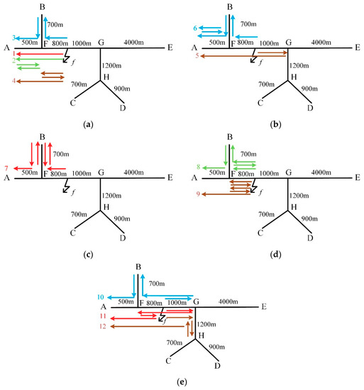
Figure 1.
Propagation paths of the fault-originated traveling waves, (a) path 1–4, (b) path 5–6, (c) path 7, (d) path 8–9, and (e) path 10–12.
In Figure 1, the arrow lines represent the TW propagation paths. Line 1 in red color shows the direct path from the fault point to A. Line 2 in green color shows the path with reflections at F and A. Line 3 in blue color shows the path with reflections at F and B. Line 4 in brown color shows the path with reflections at F and the fault point f. Similarly, multiple waves may be detected at measurement point A, which are reflected at other nodes, forming paths different from line 1–4.
As mentioned above, the propagation path of the reflected waves is longer than that of the initial wave. Moreover, the distance difference between the reflected wave and the initial wave is twice the length of the section where reflection occurs. For example, the relative distance between Line 1 and Line 2 is two times of the length of the section F–A, and it is section F–B for the case corresponding to Line 1 and Line 3. The same results can be drawn for the wave reflected at the fault point in the case involving Line 1 and Line 4 in Figure 1. Generally, there are three categories of sections:
- (1)
- Direct sections: they are included in or linked to the shortest path between the measurement point and the assumed fault section. For example, in Figure 1, if F–G is assumed as the fault section, A–F and B–F are defined as the direct sections; if G–H is assumed as the fault section, A–F, B–F, F–G and G–E are all direct sections; if A–F is assumed as the fault section, then there is no direct section.
- (2)
- Fault-originated sections: they are induced by the fault point. For example, if F–G is assumed as the fault section and the fault locates at f, then F–f and G–f are defined as the fault-originated sections; if A–F is assumed as the fault section, A–f and F–f are the fault-originated sections.
- (3)
- Indirect sections: they are linked to the direct sections or fault-originated sections. Only if the TW is reflected on the direct section or the fault-originated section, can the reflection occur on the indirect section. For example, if F–G is the fault section, G–H is an indirect section linked to the fault-originated section f–G, which is depicted as path 12 shown in Figure 1e.
2.2. Principle of the Fault-Location Method
A real distribution network can be divided into many sections by tee points and line-end points. For example, in Figure 1, the lines between two adjacent nodes are regarded as sections, forming seven sections.
In this paper, the ground and aerial mode of voltage waves were used, since voltages are easy to measure at line ends. The obtained phase voltages are decomposed into mode components through the Karrenbauer transform as depicted in Equation (1):
where V1 and V2 are the aerial modes and V0 is the ground mode. Va, Vb and Vc represent the phase voltages. One aerial mode voltage related to the faulty phase was used due to its stable velocity and small noise interference. For phase-C to the ground fault, V2 was used. For all other fault types, V1 was used.
Several time-frequency analysis methods have been developed to detect the arrival times of TWs [28,29,30,31], such as the wavelet transform and Hilbert–Huang transformation (HHT). According to [31], the HHT is conducted through two steps: empirical mode decomposition (EMD) and the Hilbert transformation. Firstly, a series of inherent modal components (named imf1, imf2,…) of the aerial-mode voltage are obtained by EMD; then, the Hilbert transform is applied to the imf1 component to explore the relationship between instantaneous frequencies (IF) and time. The first maximum of IFs indicates the arrival time of the initial wave, while other maximums indicate the arrival time of the reflected waves. A vector T is used to represent these arrival times:
where t0 is the arrival time of the initial wave and are for the reflected waves. Then, time differences can be obtained with respect to :
where is called the time difference. The corresponding results are represented by :
The index n is expected to be as large as possible to achieve a better locating result, which is related to two factors. The first one is the sampling rate. The higher the sampling rate is, the more reflected waves can be detected. However, a high sampling rate is costly to implement in practice. The other factor is that the waves being reflected several times are difficult to sense due to propagation attenuation and noise interference. With numerous simulations and experimental investigations, it has shown that an appropriate choice of n is 8–10.
With the obtained arrival time differences, the path differences between the reflected waves and the initial wave can be calculated as:
where is the ith distance difference and v is the wave velocity given in Equation (6) for a uniform overhead line [27]:
where and are the relative permittivity and magnetic permeability in free space, respectively. In the case of overhead lines, the propagation medium is air, whose relative permittivity is 1, and the wave velocity is close to the speed of light.
The calculated distance differences are listed in :
Obviously, fault location is closely related to the distance differences, which are described in relative values, and thus cannot be adopted straightforwardly to estimate the fault distance. However, is available to infer the probabilities of fault occurrence on each section, provided the networking information. The section with the largest probability will be regarded as the fault one.
The details to calculate the probability of a fault on each section are described as follows. Assuming that the distribution network was divided into k sections and n distance differences have already been obtained, a matrix was used to record the judgement results in the process of calculation.
Firstly, the probability of the fault on the assumed jth ( is randomly selected and ) section is calculated. It involves two steps:
- (1)
- For i = 1 to n (n = 10)
Based on the structure of the network, the TW undergoes multiple propagations starting from the jth section to the measurement point, forming the shortest path of the initial wave and other paths of those reflected at different sections. Herein, the essential is to figure out the specific propagation path of the reflected TW to match the calculated as depicted in Equation (5). In detail, the “distance difference” (derived from the network topology) between the specific reflected TW path starting from the jth section and the initial TW path should be equal to (here considered as being reasonable). If all the (i = 1,…, 10) are reasonable, the hypothesis that the fault is on the jth section holds. Usually, due to measurement errors and other impacts, not all the are reasonable. However, to be sure, more reasonable leads to a highly likely hypothesis.
If the ith distance difference () is reasonable, it is indicated by Jji = 1; otherwise, Jji = 0.
- (2)
- Whether the length of the fault-originated section was reasonable will be determined following the process as shown in Figure 2.
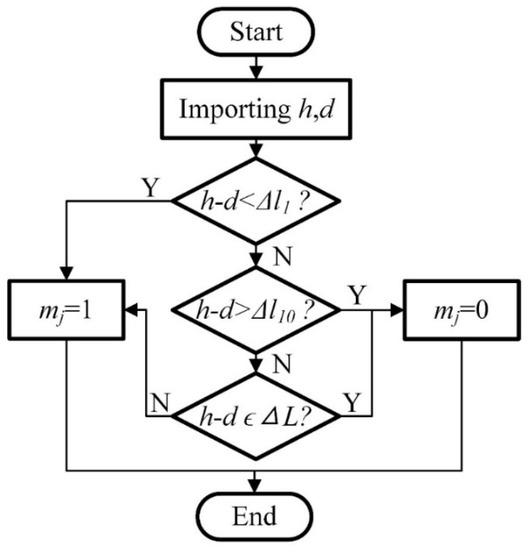 Figure 2. Flow chart to judge the rationality of the fault-originated section.
In Figure 2, h is the length of the jth section and d is the length of the fault-originated section. Obviously, if , the first distance difference should be , rather than ; if , should be included in ; and if , the length of the fault-originated section cannot judge whether it is reasonable. To avoid leaving out the true fault section, it is regarded as reasonable.
Thus, the probability of the fault on the jth section is calculated as:
Secondly, changing the index j, the aforementioned two steps are repeated until the probabilities of the fault on all k sections are obtained.
As a result, the section with the maximum probability was inferred to be the fault section. It is worth noting that a couple of sections with the same maximum probability may be determined, since numerous branches exist and the single-ended information is not sufficient. In other words, the fault location can be confined within a few sections, which greatly narrow down the scope of fault inspection for maintenance staffs. It still meets the requirement of the fast checkout of the fault locations.
Furthermore, if the unique fault section is expected, a few more measurement points can be involved, which conduct the TWs measurements independently from each other.
In practice, due to the estimation error of TW velocity, measurement errors, noise interference and other impacts, the measured distance difference () and the length of the real section (h) where reflection occurs cannot be exactly equal. Therefore, a certain level of deviation is allowed as in Equation (9):
where is selected as 15 m in this paper. In other applications, adjustments will be made to achieve better results.
2.3. Implementation Process with an Example
Supposing that a fault occurs on the section F–G, as shown in Figure 1, path 1 indicates the initial wave propagation, and the paths 2–11 represent the reflected wave propagations which are ordered from short length to long length, as shown in Figure 1.
If the path length of the initial wave is subtracted from those of the reflected ones’, 10 distance differences are obtained (they are divided by two for easy comparison with branch lengths), as listed in Table 1.

Table 1.
Distance Difference.
Then, the calculated probabilities are depicted in Table 2, where the lengths in the first row are the distance differences, as listed in Table 1. As discussed above, it is important to seek out the propagation path of the reflected TWs to match every distance difference ( to ) under each hypothesis that the fault has occurred on a certain section. It is equivalent to determine whether the distance difference can be expressed in terms of the summation of one or several “section” (among the three categories of sections described in Section 2.2) lengths.
Table 2.
Calculation of the probabilities based on the data measured at A.
Considering the second row of Table 2, the process to calculate the probability of the fault on the section A–F is explained. It is worth noting that now the fault is assumed on A–F, which means that the fault point may be A or F or any position along A–F. Obviously, if the fault point is F (the length of the fault-originated section is 0 m), the distance difference between path 2 (reflection occurs on the direct section A–F) and path 1 (the initial wave propagation path) happens to be 500 m as shown in Figure 3. Therefore, the distance difference ‘500 m’ is reasonable, indicated by a ‘√’. In the same way, ‘700 m’ is proved to be reasonable by path 3 (reflection occurs on the direct section B–F) and path 1. As for ‘800 m’, no propagation path of the TW is matched to demonstrate its reasonableness, thus it is unreasonable, indicated by a ‘○’. However, if the first unreasonable distance difference is shorter than the length of the assumed fault section, it is regarded as the length of the fault-originated section. For example, considering the probability of a fault on F–G (see the fourth row of Table 2), ‘800 m’ can be proved to be reasonable by path 4 (reflection occurs on the fault-originated section F–f) and path 1 in Figure 1a. Such a distance difference is marked by ‘√√’, which also tells the length of the fault-originated section. Similarly, the rationalities of other distance differences will be judged. Then, the value of can be obtained according to Figure 2. Finally, the probability of the fault on A–F is derived as 0.8 according to Equation (8), which is represented by ‘P’. For comparison, the probabilities of the fault on each section without such an additional judgement following Figure 2 are represented by ‘P2′.

Figure 3.
Possible traveling wave (TW) paths due to a fault at F.
From Table 2, it can be seen that F–G and E–G are both judged as the fault sections, among which F–G is the true one. If a more accurate result is required, then more measurement points are needed.
2.4. Discussion of Measurement Points Deployment
The judgement shown in Figure 2 is very useful to eliminate the falsely-determined fault sections. For example, according to ‘P2′ of Table 2, without such a judgement, F–G, G–H, D–H and E–G will be considered as fault sections. After applying the judgement, the fault sections are refined in F–G and E–G. However, it should be noted that if , the rationality of the assumed fault section cannot be determined through the judgement due to the limited number of available distance differences. As illustrated in Table 3, the judgement is effective for G–H while it is not for E–G because the length of E–G is longer than the largest distance difference. Therefore, an additional measurement device is needed at E or other feasible points to cover E–G.
Table 3.
Judgement on the different sections (G–H and E–G).
The calculated probabilities based on the data measured at E are depicted in Table 4.
Table 4.
Calculation of the probabilities based on the data measured at E.
Combining the results of Table 2 and Table 4, F–G is identified as the fault section, which is unique and consistent with the true fault section.
Since the data used are in relative values for fault location, the number of measurement points is difficult to determine. Considering the TW propagation property and complexity of the network, some empirical values are recommended. According to numerous simulations and experience from field tests in real distribution networks, 2–3 measurement points are appropriate for the medium-scale distribution networks (such as the grid shown in Figure 4). Regarding the fault location effect, measurement points would be uniformly distributed at the end of the long lines.
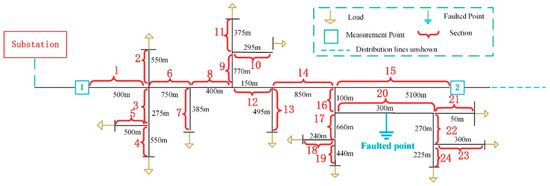
Figure 4.
Simplified distribution network.
3. Numerical Simulation
3.1. Distribution Network Modeling
Following the topology of a real distribution network of a small city in China, as shown in Figure 4, a 10 kV grid with overhead lines was modeled in PSCAD/EMTDC.
A step-down transformer at the substation was used with a voltage ratio of 110/10 kV, and the transformer was grounded through an arc suppression coil. All of the load transformers were configured in Yyn grounding mode. The type of overhead line was LGJ-35. The frequency-dependent T-Line model was adopted to model the transmission lines.
As is well known, the traveling waves will be subject to attenuation due to line loss and reflections on discontinuous nodes. Considering the propagation length of TWs, in Figure 4, parts of the real network are illustrated. Obviously, this simplification still keeps the essence of the proposed method. In addition, it implies that the fault section location can be determined independently in local areas.
3.2. Simulation Results
Two measurement points were configured in the network in order to compare the locating result of using one or more measurement points. Measurement 1# is at the beginning of the line and measurement 2# is at the end of a long-branch section as shown in Figure 4.
Assuming that a direct single-phase-to-ground fault occurs on section No.20 (120 m from the left end). The sampling rate was set to be 100 MHz. The run time of the simulation was 0.1 s and the fault occurred at 0.09 s. Measured phase voltages at point 1 and the corresponding decomposed aerial-mode voltage are shown in Figure 5.
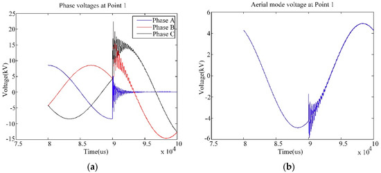
Figure 5.
Phase and aerial-mode voltages measured at point 1, (a) phase voltages, and (b) the aerial-mode voltage.
In Figure 5, it is evident that when the fault occurs, the multiple mutations appear in the voltage waves, which are caused by the arrivals of initial wave head and reflected waves. By applying the HHT to the aerial-mode voltage, the time-frequency performance can be obtained, as shown in Figure 6.
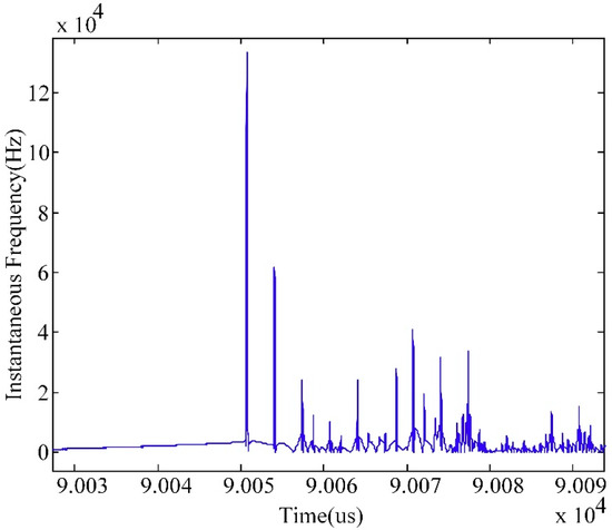
Figure 6.
Relationship between the instantaneous frequency and time.
In Figure 6, the first instantaneous frequency peak corresponds to the arrival of the fault-originated initial wave at measurement point 1, and other peaks indicate arrivals of the reflected waves. Here, the first 11 peaks are selected, resulting in 10 distance differences between the reflected waves and the initial wave according to Equations (2)–(8), thus, the probabilities of the fault happening on each section are obtained as listed in the second row of Table 5. Similarly, the measurements at point 2 can also yield the probabilities as illustrated in the sixth row of Table 5.
Table 5.
Probabilities of fault in each section.
With these two rows’ results, it is easy to figure out the fault section No. 20 by the column that takes the maximum probabilities listed in both rows, and the error of the fault distance is small. It should be noted that even if the fault section can be determined uniquely by one measurement point as Point 1, it is not always the case since it depends on the location of the potential fault. On the other hand, the sixth row of Table 5 illustrates three maximum probabilities with the same value. It means that with a single measurement point, the fault section location may be ambiguous and more measurement points will be necessary.
To further verify the effectiveness of the proposed method, a series of simulations were conducted with different assumed fault locations. The simulation results are listed in Table 6.
Table 6.
Simulation results of the different fault locations.
It is worth noting that the representation of the fault section as ‘{6,7,8}’ in Table 6 means that the fault is at the intersection of these sections. From Table 6, it is clear that if only one measurement point was used, the fault location can be confined within several sections. With more measurement points, it can effectively refine the possible fault locations.
In this paper, a high sampling rate (100 MHz) was adopted, thus the error of the fault distance was small. In Table 6, the maximum absolute error is 3.5 m, while the maximum relative error is 1.30%. It should be noted that if the fault distance is equal to the sum of the lengths of several “direct sections” (see Section 2.1) of the measurement point, it cannot be inferred by this measurement point. For example, considering the third row in Table 6, the fault is on section No.1 and the fault distance is 250 m. According to the description in Section 2.1, section No.12 and No.16 are the direct sections for measurement point 2 and the sum of their lengths is equal to the fault distance, as shown in Figure 7. Therefore, the fault distance cannot be inferred by measurement point 2, marked by ‘x’ in Table 6. However, this relationship does not hold for point 1 at this particular fault location, which means that the fault distance can still be inferred by measurement point 1.
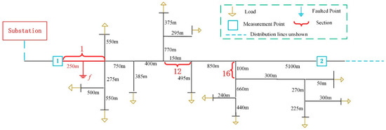
Figure 7.
Relationship between the fault distance and lengths of direct sections.
In addition, if each measurement point yields several fault sections but cannot infer the fault distance, the fault is very likely to be at the junction of these sections, which can be concluded from the last four rows in Table 6.
3.3. Impact of Transition Resistance
To investigate the effect of the transition resistance on locating results, a series of simulations were conducted under different transition resistances (150 Ω, 1000 Ω). Simulation results are listed in Table 7.
Table 7.
Simulation results under different transition resistances.
From Table 7, it can be seen that locating results under 150 Ω and 1000 Ω transition resistances are exactly the same as that of the direct ground fault. It shows that the proposed method was not affected by the transition resistance. However, with the increase in transition resistance, the mutation at fault instant decreases, as can be seen by comparing Figure 8 with Figure 5b.
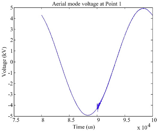
Figure 8.
The aerial-mode voltage under 1000 Ω transition resistance.
3.4. Impact of Fault Type and Grounding Mode
In a non-effectively grounded distribution network, due to weak fault current, it is not easy to locate a single-phase-to-ground fault. As for other types of faults or faults in directly grounded distribution networks, the fault characteristics are more evident, therefore this method is also available and will achieve satisfying locating results.
3.5. Impact of Noise
The accuracy of the proposed method depends on the accuracy of detecting the arrival time of traveling waves. Noises introduced by the power line itself will definitely influence the accuracy. According to the research in [16], each of the fault-wave recorders will exhibit a timestamping error due to noise interference. Similarly, noise effect is considered in this paper by a certain time deviation in each arrival time of TWs, and the results are shown in Table 8. It is clear that with the increase in time deviation, the error of the fault distance increases, however, the results of fault section identifications are unaffected.
Table 8.
Simulation results under different time deviations.
3.6. Impact of Fragmented Data
As described in the simulations, a series of 10 distance differences were used successively. In practice, one or more arrival times among the first 10 values might be unavailable due to the influence of noise and measurement error, etc. Therefore, to achieve satisfactory results, extra arrival time may be taken into account to compensate the destroyed values. Such fragmented data will indeed impact the resulted fault locations. For example, for the fault shown in Figure 4, 14 arrival times of the reflected waves were measured at Point 1 (the unique measurement point) and eight cases are considered as depicted in Table 9.
Table 9.
Locating results with discontinuous measured data.
In Table 9, the first row indexes the arrival times of the initial wave and the reflected waves. The symbol ‘√’ indicates that the indexed time contributes to the determination of the fault section. Corresponding results are shown in the last two columns. It can be seen that with more arrival times among the first 10 measures being compensated by extra time measures, greater ambiguity appears causing multiple resulting fault sections. However, the correct identification, section No.20, is always involved. Therefore, the proposed method would still work well in the condition in which sufficient but not successive reflected TWs are available.
4. Experiments Validation
To verify the practicability of the proposed method, the field tests of single-phase-to-ground faults were carried out in a real 10 kV distribution network. The topology of the distribution network is the same as shown in Figure 4.
4.1. Measurement Setup
Without a loss of generality, only one measurement point (point 1) was considered as shown in Figure 4.
As shown in Figure 9, in order to avoid the attenuation of traveling waves passing through the transformer, the measurement device was installed on the high voltage side. A capacitive voltage transformer (CVT) was used to convert the high voltage TWs into low voltage signals. A Tektronix MDO 3024 oscilloscope (OSC) was used to acquire and record traveling waves with a sampling rate of 125 MHz, which was different from 100 MHz for simulations because the oscilloscope does not have such a sampling rate configuration.
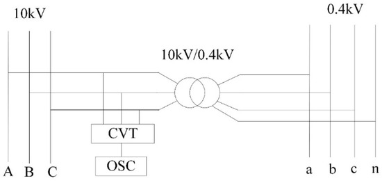
Figure 9.
The wiring diagram of a traveling-wave measurement device.
Single-phase-to-ground faults were performed at two different locations. One is on section No.20 as shown in Figure 4 and the other is on section No.14. The wiring diagram at the ground point is illustrated in Figure 10.
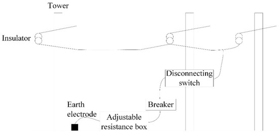
Figure 10.
The wiring diagram at the grounding point.
In Figure 10, a breaker is used to trigger the ground fault. An adjustable resistance box is configured with three ground resistances as 0 Ω, 150 Ω and 1000 Ω.
4.2. Measurement Results
When a single-phase-to-ground fault (the ground resistance is 0 Ω) occurs on section No.20, the traveling waveforms recorded by the oscilloscope are shown in Figure 11.
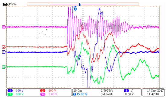
Figure 11.
TWs captured through the oscilloscope.
In Figure 11, channel 1–3 record the voltages of phase A, B, and C, among which B is the faulty phase. In addition, channel 4 is used for the transformer shell, which serves as the trigger signal for TWs recording. It has to be clarified that in Figure 11, the displayed 2.5 GS/s sampling rate is for a zoom-in demonstration. The real sampling rate is still 125 MHz. The waveform of the aerial mode voltage was derived, as shown in Figure 12.
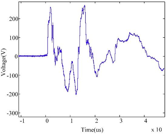
Figure 12.
The aerial-mode component of the measured voltages.
From Figure 12, it can be seen that after 20 us, the traveling wave attenuated severely, leading to difficulty in the reflected waves’ detection. In this case, the data measured within 20 us were used.
The results of the fault section location are listed in Table 10 for the cases of a fault occurring on section No.20 and section No.14. In both cases, the fault location can be confined within three sections including the true fault section with a small fault distance error. Moreover, the proposed approach was still effective in the condition of transition resistance up to 150 Ω.
Table 10.
Determination of the fault on section No.20 and No.14.
5. Discussions
Several applicable issues related to this proposed method will be discussed in this section.
5.1. Cost of Measurement Devices
To achieve accurate locating results, the sampling rate adopted is up to 100 MHz, and a CVT is used to transform the voltage traveling waves during experiments. Hence, it is necessary to compare the cost of the devices used in the proposed method with others such as the synchronous two-terminal method. In fact, although the cost of a high-sampling rate device and a CVT is higher than that of a relatively low-sampling rate device plus a synchronized device, the number of devices required varies greatly. Taking the distribution network shown in Figure 4 as an example, only two sets of the devices were required. According to the literature [16], the synchronous two-terminal scheme may use 14 sets of devices, which are installed at each line terminal. Therefore, considering the total cost, the proposed method’s consumption is not so high.
5.2. Nonhomogeneous Structure of the Distribution Network
In nonhomogeneous distribution networks, where cables have different cross-sections and various types, the proposed method is still applicable in an equivalent homogeneous network. As shown in Figure 13, M–A and N–B represent the overhead lines on which the TW propagation velocity is v1, while A–B represents a cable and the wave velocity is v2.
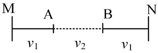
Figure 13.
Hybrid structure of the overhead lines and a cable.
The structure can be equivalent to a homogeneous overhead line by converting the actual length of A–B () into the length of the equivalent overhead line () according to Equation (10):
Thus, fault locating can be carried out for this equivalent overhead line, and the real fault distance can be obtained simply by a reverse transformation.
5.3. Use in Large-Scale Distribution Networks
In large-scale distribution networks with numerous branches and long lines, e.g., 30–50 km, the detection of TWs’ characteristics becomes much challenging because of the severe propagation attenuation. One possible way is to divide the network into small regions in the scale similar to the distribution network discussed in this paper. In each small network, the attenuation will not affect the TWs detection. Combining the section locating results of each small network, real fault location in the large-scale network can be determined.
6. Conclusions
Single-phase-to-ground fault location is a long-history problem in non-effectively grounded distribution networks, in China. The proposed fault location method takes advantage of the information of multiple reflected TWs and the prior knowledge of the network topology, thus forming an independent single-ended TW measurement scheme. In a medium-scale distribution network covering 7–8 km with multiple branches, 2–3 measurement points were sufficient to uniquely identify the fault section. Both simulations and field measurements have validated the effectiveness of the proposed method that every measurement point can provide an asynchronous judgement for the possible fault sections, resulting in a unique consequence by taking them all into account.
Author Contributions
Conceptualization, T.Z.; data curation, T.Z., Y.S. and C.Y.; formal analysis, T.Z., Y.S. and C.Y.; funding acquisition, T.Z.; investigation, T.Z., Y.S. and C.Y.; methodology, T.Z. and Y.S.; project administration, T.Z.; resources, T.Z.; software, T.Z. and Y.S.; validation, T.Z.; visualization, Y.S. and C.Y.; writing—original draft, Y.S. and C.Y.; writing—review and editing, T.Z., Y.S. and C.Y. All authors have read and agreed to the published version of the manuscript.
Funding
This work was supported in part by the Key Project of Smart Grid Technology and Equipment of National Key Research and Development Plan of China. Project No. 2017YFB0902900.
Conflicts of Interest
The authors declared that there is no conflict of interest.
Abbreviations
| CVT | Capacitive voltage transformer |
| EMD | Empirical mode decomposition |
| HHT | Hilbert–Huang transformation |
| IF | Instantaneous frequencies |
| OSC | Oscilloscope |
| TW | Traveling wave |
References
- Wang, D.; Ning, Y.; Zhang, C. An Effective Ground Fault Location Scheme Using Unsynchronized Data for Multi-Terminal Lines. Energies 2018, 11, 2957. [Google Scholar] [CrossRef]
- Dashti, R.; Sadeh, J. Fault section estimation in power distribution network using impedance-based fault distance calculation and frequency spectrum analysis. IET Gener. Transm. Distrib. 2014, 8, 1406–1417. [Google Scholar] [CrossRef]
- Salim, R.H.; Salim, K.C.O.; Bretas, A.S. Further improvements on impedance-based fault location for power distribution systems. IET Gener. Transm. Distrib. 2011, 5, 467–478. [Google Scholar] [CrossRef]
- Bayati, N.; Baghaee, H.; Hajizadeh, A.; Soltani, M. Localized Protection of Radial DC Microgrids with High Penetration of Constant Power Loads. IEEE Syst. J. 2020, 1–12. [Google Scholar] [CrossRef]
- Majidi, M.; Etezadi-Amoli, M. A New Fault Location Technique in Smart Distribution Networks Using Synchronized/Nonsynchronized Measurements. IEEE Trans. Power Deliver. 2018, 33, 1358–1368. [Google Scholar] [CrossRef]
- Jia, K.; Bi, T.; Ren, Z.F.; Thomas, D.W.P.; Sumner, M. High frequency impedance based fault location in distribution system with DGs. IEEE Trans. Smart Grid 2018, 9, 807–816. [Google Scholar] [CrossRef]
- Krishnathevar, R.; Ngu, E.E. Generalized impedance-based fault location for distribution systems. IEEE Trans. Power Deliver. 2012, 27, 449–451. [Google Scholar] [CrossRef]
- Baghaee, H.; Mlakić, D.; Nikolovski, S.; Dragicevic, T. Support Vector Machine-based Islanding and Grid Fault Detection in Active Distribution Networks. IEEE J. Em. Sel. Top. Power Syst. 2019, 1–19. [Google Scholar] [CrossRef]
- Liang, R.; Peng, N.; Zhou, L.; Meng, X.; Hu, Y.; Shen, Y.; Xue, X. Fault Location Method in Power Network by Applying Accurate Information of Arrival Time Differences of Modal Traveling Waves. IEEE Trans. Ind. Inform. 2020, 16, 3124–3132. [Google Scholar] [CrossRef]
- Gale, P.F.; Crossley, P.A.; Bingyin, X.; Yaozhong, G.; Cory, B.J.; Barker, J.R.G. Fault location based on travelling waves. In Proceedings of the 1993 Fifth International Conference on Developments in Power System Protection, York, UK, 30 March–2 April 1993; pp. 54–59. [Google Scholar]
- Magnago, F.H.; Abur, A. Fault location using wavelets. IEEE Trans. Power Deliver. 1998, 13, 1475–1480. [Google Scholar] [CrossRef]
- Lopes, F.V.; Silva, K.M.; Costa, F.B.; Neves, W.L.A.; Fernandes, D. Real-Time Traveling-Wave-Based Fault Location Using Two-Terminal Unsynchronized Data. IEEE Trans. Power Deliver. 2015, 30, 1067–1076. [Google Scholar] [CrossRef]
- Marihart, D.J.; Haagenson, N.W. Automatic fault location for Bonneville Power Administration. In Proceedings of the IEEE/PES Summer Meeting, San Francisco, CA, USA, 9–14 July 1972; pp. 1–6. [Google Scholar]
- Lee, H.; Mousa, A.M. GPS travelling wave fault locator systems: Investigation into the anomalous measurements related to lightning strikes. IEEE Trans. Power Deliver. 1996, 11, 1214–1223. [Google Scholar] [CrossRef]
- Robson, S.; Haddad, A.; Griffiths, H. Fault Location on Branched Networks Using a Multiended Approach. IEEE Trans. Power Deliver. 2014, 29, 1955–1963. [Google Scholar] [CrossRef]
- Goudarzi, M.; Vahidi, B.; Naghizadeh, R.A.; Hosseinian, S.H. Improved fault location algorithm for radial distribution systems with discrete and continuous wavelet analysis. Int. J. Elec. Power 2015, 67, 423–430. [Google Scholar] [CrossRef]
- Lopes, F.; Dantas, K.; Silva, K.; Costa, F. Accurate Two-Terminal Transmission Line Fault Location Using Traveling Waves. IEEE Trans. Power Deliver. 2017, 33, 873–880. [Google Scholar] [CrossRef]
- Lopes, F.V. Settings-Free Traveling-Wave-Based Earth Fault Location Using Unsynchronized Two-Terminal Data. IEEE Trans. Power Deliver. 2016, 31, 2296–2298. [Google Scholar] [CrossRef]
- Robson, S.; Haddad, A.; Griffiths, H. Traveling Wave Fault Location Using Layer Peeling. Energies 2019, 12, 126. [Google Scholar] [CrossRef]
- Pourahmadi-Nakhli, M.; Safavi, A.A. Path Characteristic Frequency-Based Fault Locating in Radial Distribution Systems Using Wavelets and Neural Networks. IEEE Trans. Power Deliver. 2011, 26, 772–781. [Google Scholar] [CrossRef]
- Cao, P.; Shu, H.; Yang, B.; Dong, J.; Fang, Y.; Yu, T. Speeded-up robust features based single-ended travelling wave fault location: A practical case study in Yunnan power grid of China. IET Gener. Transm. Distrib. 2018, 12, 886–894. [Google Scholar] [CrossRef]
- Lin, S.; He, Z.Y.; Li, X.P.; Qian, Q.Q. Travelling wave time-frequency characteristic-based fault location method for transmission lines. IET Gener. Transm. Distrib. 2012, 6, 764–772. [Google Scholar] [CrossRef]
- Borghetti, A.; Bosetti, M.; Di Silvestro, M.; Nucci, C.A.; Paolone, M. Continuous-Wavelet Transform for Fault Location in Distribution Power Networks: Definition of Mother Wavelets Inferred from Fault Originated Transients. IEEE Trans. Power Syst. 2008, 23, 380–388. [Google Scholar] [CrossRef]
- Borghetti, A.; Bosetti, M.; Nucci, C.A.; Paolone, M.; Abur, A. Integrated Use of Time-Frequency Wavelet Decompositions for Fault Location in Distribution Networks: Theory and Experimental Validation. IEEE Trans. Power Deliver. 2010, 25, 3139–3146. [Google Scholar] [CrossRef]
- Mardiana, R.; Motairy, H.A.; Su, C.Q. Ground Fault Location on a Transmission Line Using High-Frequency Transient Voltages. IEEE Trans. Power Deliver. 2011, 26, 1298–1299. [Google Scholar] [CrossRef]
- Benato, R.; Sessa, S.D.; Poli, M.; Quaciari, C.; Rinzo, G. An Online Travelling Wave Fault Location Method for Unearthed-Operated High-Voltage Overhead Line Grids. IEEE Trans. Power Deliver. 2018, 33, 2776–2785. [Google Scholar] [CrossRef]
- Abad, M.; García-Gracia, M.; Halabi, N.E.; Andía, D.L. Network impulse response based-on fault location method for fault location in power distribution systems. IET Gener. Transm. Distrib. 2016, 10, 3962–3970. [Google Scholar] [CrossRef]
- Hamidi, R.J.; Livani, H.; Rezaiesarlak, R. Traveling-Wave Detection Technique Using Short-Time Matrix Pencil Method. IEEE Trans. Power Deliver. 2017, 32, 2565–2574. [Google Scholar] [CrossRef]
- Moravej, Z.; Movahhedneya, M.; Radman, G.; Pazoki, M. Effective fault location technique in three-terminal transmission line using Hilbert and discrete wavelet transform. In Proceedings of the IEEE International Conference on Electro/Information Technology (EIT), Dekalb, IL, USA, 21–23 May 2015; pp. 170–176. [Google Scholar] [CrossRef]
- Bernadić, A.; Leonowicz, Z. Determining of fault location with Hilbert—Huang transformation on XLPE cables between land and offshore substations. In Proceedings of the 14th International Conference on Environment and Electrical Engineering, Krakow, Poland, 10–12 May 2014; pp. 61–64. [Google Scholar]
- Yang, W.; Xiangjun, Z.; Xiaoan, Q.; Zhenfeng, Z.; Hui, P. HHT based single terminal traveling wave fault location for lines combined with overhead-lines and cables. In Proceedings of the International Conference on Power System Technology, Hangzhou, China, 24–28 October 2010; pp. 1–6. [Google Scholar] [CrossRef]
© 2020 by the authors. Licensee MDPI, Basel, Switzerland. This article is an open access article distributed under the terms and conditions of the Creative Commons Attribution (CC BY) license (http://creativecommons.org/licenses/by/4.0/).