Abstract
The identification of underground formation lithology can serve as a basis for petroleum exploration and development. This study integrates Extreme Gradient Boosting (XGBoost) with Bayesian Optimization (BO) for formation lithology identification and comprehensively evaluated the performance of the proposed classifier based on the metrics of the confusion matrix, precision, recall, F1-score and the area under the receiver operating characteristic curve (AUC). The data of this study are derived from Daniudui gas field and the Hangjinqi gas field, which includes 2153 samples with known lithology facies class with each sample having seven measured properties (well log curves), and corresponding depth. The results show that BO significantly improves parameter optimization efficiency. The AUC values of the test sets of the two gas fields are 0.968 and 0.987, respectively, indicating that the proposed method has very high generalization performance. Additionally, we compare the proposed algorithm with Gradient Tree Boosting-Differential Evolution (GTB-DE) using the same dataset. The results demonstrated that the average of precision, recall and F1 score of the proposed method are respectively 4.85%, 5.7%, 3.25% greater than GTB-ED. The proposed XGBoost-BO ensemble model can automate the procedure of lithology identification, and it may also be used in the prediction of other reservoir properties.
1. Introduction
Lithology identification plays a crucial role in the exploration of oil and gas reservoirs, reservoir modelling, drilling planning and well completion management. Lithology classification is the basis of reservoir characterization and geological analysis. It is possible to generate lithological patterns after being informed of lithology. Such patterns can be applied in simulators for the purpose of understanding the potentiality of an oil field. Apart from the significance in geological studies, lithology identification also has practical value in enhanced oil recovery processes and well planning [1,2,3,4].
Many researches have been done on lithology identification, which is mainly divided into two parts: direct and indirect. The direct methods to determine the lithology are to make inferences from core analysis and drilling cuttings [5,6]. However, it is expensive, time-consuming and not always reliable since different geologists may provide different interpretations [7]. Compared with the direct method, using well logs to identify lithology is a universal indirect method, which is more accurate, effective and economical. Until now, there have been many lithology identification methods associated with logs, including the cross plotting method, traditional statistical analysis and several machine learning methods [8,9,10]. The cross plotting takes a considerable amount of time of an experienced analyst, especially in the heterogeneous reservoir. Due to the high dimensional, non-linear and noisy characteristics of well log data, traditional statistical methods, such as histogram plotting and multivariable statistical analysis, are difficult to identify lithology accurately [11]. Therefore, robust, efficient and accurate predictive techniques are required in the formation lithology identification. At present, machine learning is becoming a vital instrument to predict lithology with well log data. Machine learning can analyze the high dimensional and non-liner well log data and make the process of the lithology identification more efficient and intelligent.
Several machine learning techniques have been introduced to lithology identification. They are mainly divided into unsupervised learning and supervised learning. A variety of unsupervised learning approaches to the problem of lithology prediction based on well log data have been applied over the past few decades. Konaté et al. combined cross-plot and principal component analysis (PCA) methods to extract the critical information of lithology identification [12]. Yang et al. performed a synergetic wavelet transform and modified K-means clustering techniques in well logs to classify lithology [13]. Bhattacharya et al. applied Multi-Resolution Graph-based Clustering to reduce the uncertainty of propagating single-well based lithology prediction [14]. Shen et al. used wavelet analysis and PCA to handle lithology identification [15]. Unsupervised learning can classify lithology based on the characteristics of the data, but the accuracy is usually lower than supervised learning. It can be better as an exploratory technique if the geology is unknown. In recent years, supervised learning methods are frequently prescribed for lithology identification. Ren et al. applied artificial neural networks (ANN) to calculate the lithology probabilities [16]. Wang et al. applied support vector machine (SVM) and ANN in recognizing shale lithology based on well conventional logs and suggested that SVM is superior to ANN [17]. Sun et al. proposed that Random Forest (RF) had higher accuracy and consumed less time than SVM [18]. Xie et al. comprehensively compared the performance of five machine learning methods and concluded that Gradient Tree Boosting (GTB) and RF had better accuracy than the other three methods [19].
It is worth noting that RF and GTB belong to ensemble methods, and they are the heated topic in the field of supervised learning. However, a more efficient ensemble method called Extreme Gradient Boosting (XGBoost) has rarely been reported in lithology recognition. Moreover, the performance of data-driven methods depend on the parameters, and the values of parameters should be adjusted to acquire proper estimations. Grid search is the most widely used parameter optimization algorithm nowadays, but this method relies on the optimization by the traversing of all parameters, which costs a lot in the calculation process. Besides, grid search needs to sample in multiple same internals for continuous data, where the global optimum cannot always be achieved [20]. To deal with this problem, the Bayesian Optimization algorithm (BO), an emerging optimization algorithm based on probability distribution in recent years, is introduced.
BO can obtain the optimal solution of a complex objective function in a few evaluations. Ghahramani et al. pointed out that BO is one of the most advanced, hopeful techniques in probabilistic machine learning and artificial intelligence fields [21].
This study proposes XGBoost classifier combined with BO algorithm for formation lithology identification. Simultaneously, in order to more comprehensively evaluate the performance of our learning model, the effect of lithology identification, the performance of the algorithm is evaluated based on the metrics of classification accuracy, confusion matrix, precision, recall, F1-score and the area under the receiver operating characteristic curve (AUC) have been used for estimation. Additionally, we compare the proposed algorithm with those in the literature using the same dataset, which are GTB and GTB with ED.
2. Materials and Methods
2.1. Studied Data
The studied area is located in the Ordos Basin in the central west of China (Figure 1), which is the main producing area of natural gas in China.
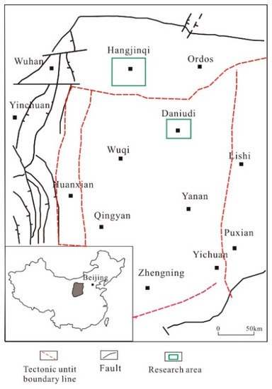
Figure 1.
Locations of the study area and the studied sections.
The relevant research data are collected from two gas fields in Ordos Basin, namely, Daniudi gas field (DGF) and Hangjinqi gas field (HGF) [19]. The dataset we used is log data from twelve wells (with 2153 examples) that have been labelled with a lithology type based on observation of core. This dataset consists of a set of eight predictor variables and a lithology class for each example vector. Predictor variables include seven from well log measurements and corresponding depth. The seven log properties include: acoustic log (AC), caliper log (CAL), gamma ray log (GR), deep latero log (LLD), shallow latero log (LLS), density log (DEN) and compensated neutron (CNL). The sampling frequency of well logs is 0.125 m.
Due to the complex geological structure, the tectonic development of the target layer and real-time logging data captured by sensors are noisy, which causes a certain particular deviation in the measurement results. Therefore, data preprocessing is required before using a machine learning algorithm.
Using the Tukey’s method to detect outliers is a standard method of noise reduction. In this method, the sequence has been divided into four parts, and then it is required to find the first quartiles and third quartiles [22]. The interquartile range (IQR) is calculated by Equation (1). Lower Inner Fence (LIF) and Upper Inner Fence (UIF) have been calculated through Equations (2) and (3). All the values outside of LIF and UIF are considered as outliers and should be eliminated. The data is shown in Table 1.

Table 1.
Statistical details about the well logs in this article.
The core analyses report that the lithology classes are composed of clastic rocks, carbonate rock (CR) and coal (C). According to the detrital grain size classification of Chinese oil industry [23], the clastic rocks in this research are divided into six types, namely, pebbly sandstone (PS) (>1 mm grain size), coarse sandstone (CS) (0.5–1 mm grain size), medium sandstone (MS) (0.25–0.5 mm grain size), fine sandstone (FS) (0.01–0.25 mm grain size), siltstone (S) (0.005–0.05 mm grain size), and mudstone (M) (<0.005 mm grain size). The number of samples in each class for the research areas could be presented, as shown in Figure 2.
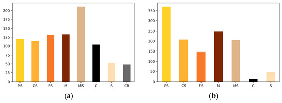
Figure 2.
The number of samples in each class for the research areas: (a) The distribution of lithologies in the Daniudi gas field (DGF); (b) the distribution of lithologies in the Hangjinqi gas field (HGF).
2.2. Methods
2.2.1. Extreme Gradient Boosting
XGBoost algorithm is a lifting algorithm that generates multiple weak learners by continuous residual fitting, which belongs to a kind of ensemble learning. The accumulation of weak learners will produce a strong one in the end. In the optimizing process, XGBoost uses Taylor expansion to introduce the information of the second derivative as loss functions, so the model has a faster convergence speed. Besides, to prevent overfitting, XGBoost added regularization terms in loss functions to inhibit the complexity of the model [24].
Assuming is a data integration, including samples with each sample having eigenvalues, whereas represents the value of sample . The classification and regression tree (CART) is selected as the base model, then the integrated model of XGBoost composes (number of trees) base models into an addition expression to predict the final result [25].
The prediction precision of the model is determined together by deviation and variance, while the loss function can reflect the deviation of the model. To control the variance and simplify the model, regularization terms are added to inhibit the model complexity. Together with the loss functions of the model, objective functions of XGBoost functions are constituted as following.
where is the objective function of tree , is the summation of the output values of the previous trees, is the output value of tree , is the differentiable convex loss function to balance the prediction value and true value . is the penalty term representing model complexity, is the regularization parameter representing the leaf number, is the regularization parameter representing the leaf weights and is the value of a leaf node. Define as the sample set of leaf set , then expand the loss functions with Taylor series at . Define and as the first derivative and second derivative of Taylor expansions, respectively, then remove the constant term, so the loss function after iterations becomes
where is the weight of leaf node . Define and then substitute them into Equation (6), so the objective function can be simplified as
In the above equation, leaf node is an uncertain value, so take the first derivative of objective function with respect to and the optimal value of leaf node can be obtained.
Substitute back into the objective function, so the minimum value of can be calculated as
2.2.2. Bayesian Optimization
Unlike other optimization algorithms, BO constructs a probability model of functions to be optimized and utilizes the model to determine next point that requires evaluation. The algorithm assumes a collection function according to the prior distribution, while the new sampling sites are used to test the information of objective functions to update the prior distribution. Then most possible locations for the global values (given by posterior distribution) are tested. It can be seen that although BO algorithm needs to operate more iterations to confirm that next sampling point, fewer evaluations are required to find the minimum of a complex convex function [26].
There are two important procedures when operating BO algorithm. First, a transcendental function needs to be selected to show the distribution hypothesis of the optimized function. This procedure usually utilizes the Gaussian process, which is highly flexible and trackable. Then, an acquisition function is required to construct a utility function from the model posterior distribution, so next point could be determined to evaluate.
Gaussian Process refers to a set of random variables. In this paper, it represents different parameter combinations in the XGBoost algorithm, whereas the linear combinations with any limited samples have a joint Gaussian Process [27].
where , is the mathematical expectation, is the covariance function of and MAE is the mean absolute error of , the formula of which is
In the formula, refers to the predicted output of XGBoost and represents the true error when calculating the result under current influence factors. One of the characteristics of Gaussian Process is every related with , while for a set , there is a joint Gaussian Process satisfying the formula below
If a pair of known samples is added into the new sample , the joint Gaussian Process expresses as
Calculate the posterior probability of with Equations (13) and (14) as
After inputting the sample combination points into the Gaussian model, so the mean value and variance of can be gained. If the sample points increase gradually, the gap between posterior probability and true value of will be narrowed a lot. The target of defining an extract function is to extract sampling points in parameter space with purposes, while there are two directions to extract those points [28].
- (1)
- Explore. Select unevaluated parameter combinations as much as possible to avoid local optimal values, so the posterior probability of will reach the true value of .
- (2)
- Exploit. Based on the optimal values found, after searching the parameters around, the global optimum can be found faster.
Probability of Improvement (POI) function is chosen as the acquisition function. The basic idea of this method is to maximize the probability when the point to be selected next step improves the maximum. If the current found maximum is , then the extract function is listed as below:
In which refers to the normal cumulative distribution function, which is also called maximum probability of improvement (MPI).
From Formula (18) it can be seen that the function turns to select the parameter combinations around the known optimal values. To make the algorithm explore more unknown space as much as possible, a trade-off function is added. In this case, it can be avoided to search the optimal values near to and the coefficient can be altered dynamically to control the direction to find the optimal values: Either in the explore direction or exploit direction.
BO algorithm aims to find the in the set and make the unknown function reach the global maximum or minimum. The selection of follows
2.2.3. Details of Implementation
The dataset were randomly split into a training set and test set through the cross-validation. The iteration process of our proposed ensemble algorithm is shown in Figure 3.
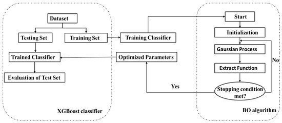
Figure 3.
The procedure of the proposed ensemble technique.
The first step is to randomly generate initialization points based on the number and range of XGBoost hyperparameters. The next step is to input the initialization parameters into the Gaussian Process and modify them. Then we use the extract function to select the combined parameters to be evaluated from the modified Gaussian process. If the error of the newly chosen combined parameters meets the target requirements, the algorithm execution is terminated, and the corresponding combined parameters are output. We use this set of parameters to obtain the trained classifier and evaluate the classifier through the test set. If the target requirements are not met, modify the Gaussian Process until the set conditions are satisfied.
3. Performance Measure
Not only does the generalization performance evaluation of this lithology classifier requires an effective and feasible experimental estimation method, but also a standard to measure the generalization ability of the model, which is the performance measurement. The performance of each task was measured using different metrics, which depends on the task. When comparing the capabilities of varying lithology classifiers, different performance metrics often leads to different judgment results.
In order to more comprehensively evaluate the effect of performance of our model, we used the following metrics: accuracy, confusion matrix, precision, recall, F1-score, and the area under the receiver operating characteristic curve.
The accuracy, given by Equation (20), measures the percentage of the correct classification by comparing the predicted classes with those classified by the manual method.
where is the predicted lithology classes of test samples and is the correct classification of this sample. If then , otherwise .
According to the combination of exact lithology classes and algorithm prediction classes, the sample is divided into four cases: true positive (TP), false positive (FP), true negative (TN), and false negative (FN).
The recall is defined in Equation (21).
The recall indicates that the percentage of true positive samples that are classified as positive. The precision is defined in Equation (22).
The precision measures the proportion of actual positive samples among the samples that are predicted to be positive.
The F1 score is the harmonic mean of Recall and Precision. The F1 score can be calculated as:
Receiver Operating Characteristics (ROC) curve is used to evaluate generalization performance, and the area of the curve is AUC. The ROC curve is acquired by the true positive rate (TPR) and the false positive rate (FPR) at assorted discrimination levels [29]. The TPR and FPR can be written as (24) and (25).
The AUC value varies from 0.5 to 1, and there are different standards in various situations. In medical diagnosis, a very high AUC (0.95 or higher) is usually required, while other domains consider that 0.7 AUC value has a strong effect [30].
4. Results and Discussion
This section comprehensively evaluates the lithology identification results of the XGBoost combined with BO. At first, the search process and BO results of the best parameters value set for XGBoost are presented. Furthermore, the evaluation matrix that contains accuracy, confusion matrix, precision, recall, F1-score and AUC is assessed over the model trained with the best hyperparameter in XGBoost classifier. Finally, we compare our studies with previous academics’ studies in two areas using the same data.
4.1. Tuning Process
The optimum parameter settings used in BO for XGBoost model selection are shown in Table 2.
Table 2.
Tuned parameters for XGBoost and tuned optimum parameter value in the DFG and HGF.
The Number of estimators were randomly chosen in the interval [10, 100]. The Max depth was randomly chosen in the interval [1, 20]. The Learning rate was chosen from a uniform distribution ranging from 1 × 10⁻³ to 5 × 10⁻¹. The Subsample was randomly chosen in the interval [0.1, 1]. The Min child weight was randomly chosen in the interval [1, 10]. The Gamma was randomly chosen in the interval [0.1, 0.6]. The Colsample bytree was randomly chosen in the interval [0.5, 1]. The Reg alpha was chosen from a uniform distribution ranging from 1 × 10⁻⁵ to 1 × 10⁻². The objective function is accuracy. Moreover, the max eval of the optimization function is set as 300. We use the data from DGF and HGF to determine the parameters for each gas field. The tuned optimum parameters are shown in Table 2.
To appraise the efficiency of the proposed approach, consider four levels for each one of the eight parameters. The grid search technique generates 48 = 65,536 candidate settings, while the BO generations require 300 model evaluations, representing 0.45% of the budget of the grid search technique. In order to reflect the Bayesian Optimization process more intuitively, taking HGF data as an example, the XGBoost algorithm parameters tuning process by BO are shown in Figure 4.
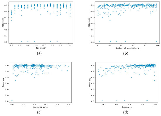
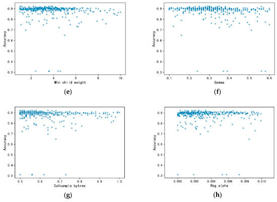
Figure 4.
The XGBoost parameters tuning process by BO. (a) Max depth tuning process; (b) number of estimators tuning process; (c) learning rate tuning process; (d) subsample tuning proces€(e) minimum child weight tuning process; (f) gamma tuning process; (g) consample bytree tuning process; (h) reg alpha tuning process.
BO makes full use of the previous sample point’s information during parameters tuning process. The eight parameters find their optimum value with relatively fewer iterations. The search range of Max Depth is relatively uniform, due to a narrow range of parameters. The first half of the search range of the Number of Estimators is relatively dispersed, while the last half is more concentrated. The search range of Learning Rate is mainly from 0 to 0.3. Moreover, the search range of subsample is mainly from 0.8 to 1, while that of Min Child Weight is from 0 to 0.5. The search range of Gamma is relatively uniform, while that of Colsample bytree mainly focuses between 0.5 and 0.7. The search in the boundary is less for Reg alpha. Generally, Bo initiates each parameter in the whole range. After acquiring more feedbacks from objective function as times goes by, the search range mainly focuses on the possible optimum range. Although it will search in the whole space, it is not as frequent as before.
4.2. Evaluation Matrix
To acquire both steady and reliable results, learning dataset has been divided into a training set and test set using cross-validation, and then take the average of 10 independent runs as the final results. Then we averaged the scores, including precision, recall and F1-score to evaluate the performances of the model. Table 3 and Table 4 show the scores of each lithology class for the model in the DGF and HGF, respectively.
Table 3.
Performance matrix of each lithology class for 5-fold-cross-validation averaged over ten runs in the DGF.
Table 4.
Performance matrix of each lithology class for 5-fold-cross-validation averaged over ten runs in the HGF.
Table 3 and Table 4 present the mean for precision, recall and F1 produced by XGBoost combined with BO in the DGF and HGF, respectively. Overall, the results of HGF show better performance compared with DGF. This may be related to the lithology categories. Although the geological conditions of the two gas fields are similar, compared with the DGF, the HGF dataset does not have CR class instances, which may increase the risk of misclassification of lithology in the DGF. In addition, the classification of lithology C is the best in both gas fields. The main reason is that the lithology of C has a significant gap compared with other lithologies. At the same time, the CS lithology classification effect is the worst in the DGF, but has better performance in the HGF. This may be because the number of CS samples in the HGF is about twice that of DGF, and the XGBoost algorithm can learn more features in the samples, thus, enhancing the accuracy of the results.
Figure 5 presents the confusion matrix of the lithologic classes by XGBoost combined with BO in the DGF and HGF. Compared predicted classes with true exact classed by confusion matrix, it can demonstrate the misclassified lithology types.
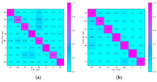
Figure 5.
Heat map of Confusion matrix on the test dataset. (a) The DGF test dataset; (b) the HGF test dataset.
In the case of the DGF test set, the accuracy of M, C, and CR is highest, which probably because the lithology difference is significant compared with others. Four percent of M were misclassified as CR, due to the deposition environment of lake sediments. The type of M is carbonate-like mud, which contains a portion of CaCO3, resulting in misclassification of CR. Besides, there is more probability of misclassification between PS, CS, FS, MS, and S. It is likely that the grain sizes of sandstone are challenging to determine, and human error is involved in the interpretation of lithology.
Overall, for the HGF test set, the accuracy of M, and C classes is higher than 90%. Especially the accuracy rate of class C is up to 100%. This may have been caused by the quite different lithology properties in C and M compared to other classes. Mistakes are also mainly concentrated in sandstone classes. Although there are significant variance between M and other lithologies, it still has 6% of M misclassified as PS. This is likely because the leaning sample is imbalanced, the PS classes have the highest proportion in the HGF. There is no misclassification in the DGF since the number of samples in M and PS is very close.
In order to evaluate the generalization performance of the proposed algorithm, the ROC curve is used here to evaluate the expected generalization performance, as shown in Figure 6.
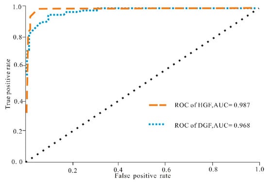
Figure 6.
ROC curves for the lithology identification based on the XGB combined with BO in the DGF and HGF; AUC, area under the ROC curve.
XGBoost can be used to calculate the TPR and FPR of the lithology to be tested at various thresholds, thereby drawing a ROC curve. In this way, a total of eight ROC curves can be drawn in the DGF, and seven ROC curves in the HGF. The ROC curves of each gas field are averaged to obtain the final ROC curves and AUC values corresponding to the gas field. The diagonal line in the figure corresponds to the random guess model, that is, the AUC value is 0.5, and the AUC value of 1 represents the ideal model. The AUC of HGF is 0.987, and the AUC of DGF is 0.968. The performance of HGF is better than DGF, and both are greater than 0.95. The proposed algorithm has a strong generalization ability in these two gas fields.
Figure 7 shows the point plots comparing the results found for lithology identification with those available in references. The dataset of this article is the same as the references. Xie et al. used five machine learning methods to identify lithology and concluded that the Gradient Tree Boosting, which belonged to the ensemble learning method for formation lithology identification had the best performance [19]. Saporetti et al. combined the Gradient Tree Boosting with a differential evolution to identify lithology [31].
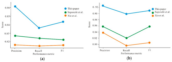
Figure 7.
Point plots for results produced by the proposed approach compared with references. (a) The DGF dataset; (b) the HGF dataset.
The scatter plot represents the average value of the calculated results. It can be seen from Figure 7 that the three evaluation indexes of precision, recall and F1 score of the proposed method are significantly greater than those of the references. In the DGF, there is little difference between the three indicators in the reference. The proposed method has a significant improvement effect on the results of precision, the performance improvement is significantly higher than the others, and the recall improvement is relatively minimal. In the HGF, the increase of precision and recall is similar, and both are higher than the F1 score. The three indexes have significant improvements in the HGF. Precision and Recall have the biggest improvements, and they are much closer to each other. Compared with DGF, the improvement of our proposed model is much more significant, which probably because the sample dataset is more enough in the HGF and our model can extract more features. The improvement of lithology identification accuracy can promote the accuracy of our geological model effectively. Based on geological model, it is better and more precise to calculate the geological reserves. With more accurate lithology identification, it is better to optimize well placement and perforating location, as well as obtain higher drilling encountering rate and higher production.
5. Conclusions
In this study, in order to simplify the data-driven pipeline for formation lithology classification, we investigated the use of the BO in search of the optimal hyperparameters of the XGBoost classifier based on well log data. To acquire both steady and reliable results, learning dataset has been divided into a training set and test set using cross-validation, and then take the average of 10 independent runs as the final results.
In addition, we comprehensively evaluated the performance of the proposed classifier. The AUC values of the test sets of the DGF and HGF fields are 0.968 and 0.987, respectively, indicating that the proposed method has very high generalization performance. The averaged results of Precision, Recall, and F1 score of our method are respectively 5.9%, 5.7%, 6.15% greater than those of GTB, while 4.85%, 5.7%, 3.25% higher than those of GTB-DE.
Furthermore, the proposed classifier can assist the geologist to accurately and efficiently identify the formation lithology. Specialists can make use of the XGBoost model to analyze a large amount of well log data during geological exploration, such as the estimation of fracture density, the prediction of reservoir permeability and the calculation of porosity, which can improve the data analysis efficiency in petroleum geology.
Author Contributions
Conceptualization, Z.S. and B.J.; methodology, Z.S. and B.J.; software, B.J.; validation, Z.S., X.L. and J.L.; formal analysis, Z.S., B.J. and X.L; investigation, Z.S., B.J. and J.L.; resources, Z.S.; data curation, Z.S. and K.X.; writing—original draft preparation, B.J.; writing—review and editing, Z.S. and B.J.; visualization, X.L. and J.L.; supervision, Z.S. and B.J.; project administration, K.X.; funding acquisition, Z.S. All authors have read and agreed to the published version of the manuscript.
Funding
This study was jointly supported by the National Natural Science Foundation of China (Grant NO.51774317), the Fundamental Research Funds for the Central Universities (Grant No.18CX02100A) and National Science and Technology Major Project (Grant NO.2016ZX05011004-004).
Acknowledgments
We are grateful to all staff involved in this project, and also wish to thank the journal editors and the reviewers whose constructive comments improved the quality of this paper greatly.
Conflicts of Interest
The authors declare that they have no conflict of interest.
Abbreviations
| XGBoost | Extreme Gradient Boosting |
| BO | Bayesian Optimization |
| AUC | Rceiver operating characteristic curve |
| GTB-DE | Gradient Tree Boosting-Differential Evolution |
| PCA | Principal component analysis |
| ANN | Artificial neural networks |
| SVM | Support vector machine |
| RF | Random Forest |
| DGF | Daniudi gas field |
| HGF | Hangjinqi gas field |
| AC | Acoustic log |
| CAL | Caliper log |
| GR | Gamma ray log |
| LLD | Deep latero log |
| LLS | Shallow latero log |
| DEN | Density log |
| Q1 | The first quartiles |
| Q3 | The third quartiles |
| IQR | The interquartile range |
| LIF | Lower Inner Fence |
| UIF | Upper Inner Fence |
| CR | Carbonate rock |
| C | Coarse sandstone |
| PS | Pebbly sandstone |
| CS | Coarse sandstone |
| MS | Medium sandstone |
| FS | Fine sandstone |
| S | Siltstone |
| M | Mudstone |
| TP | True positive |
| FP | False positive |
| TN | True negative |
| FN | False negative |
| ROC | Receiver operating characteristics |
| TPR | True positive rate |
| FPR | False positive rate |
References
- Chen, G.; Chen, M.; Hong, G.; Lu, Y.; Zhou, B.; Gao, Y. A New Method of Lithology Classification Based on Convolutional Neural Network Algorithm by Utilizing Drilling String Vibration Data. Energies 2020, 13, 888. [Google Scholar] [CrossRef]
- Santos, S.M.G.; Gaspar, A.T.F.S.; Schiozer, D.J. Managing reservoir uncertainty in petroleum field development: Defining a flexible production strategy from a set of rigid candidate strategies. J. Pet. Sci. Eng. 2018, 171, 516–528. [Google Scholar] [CrossRef]
- Liu, H.; Wu, Y.; Cao, Y.; Lv, W.; Han, H.; Li, Z.; Chang, J. Well Logging Based Lithology Identification Model Establishment Under Data Drift: A Transfer Learning Method. Sensors 2020, 20, 3643. [Google Scholar] [CrossRef] [PubMed]
- Obiadi, I.I.; Okoye, F.C.; Obiadi, C.M.; Irumhe, P.E.; Omeokachie, A.I. 3-D structural and seismic attribute analysis for field reservoir development and prospect identification in Fabianski Field, onshore Niger delta, Nigeria. J. Afr. Earth Sci. 2019, 158, 12. [Google Scholar] [CrossRef]
- Saporetti, C.M.; da Fonseca, L.G.; Pereira, E.; de Oliveira, L.C. Machine learning approaches for petrographic classification of carbonate-siliciclastic rocks using well logs and textural information. J. Appl. Geophys. 2018, 155, 217–225. [Google Scholar] [CrossRef]
- Logging, C. Reservoir characteristics of oil sands and logging evaluation methods: A case study from Ganchaigou area, Qaidam Basin. Lithol. Reserv. 2015, 27, 119–124. [Google Scholar]
- Harris, J.R.; Grunsky, E.C. Predictive lithological mapping of Canada’s North using Random Forest classification applied to geophysical and geochemical data. Comput. Geosci. 2015, 80, 9–25. [Google Scholar] [CrossRef]
- Vasini, E.M.; Battistelli, A.; Berry, P.; Bonduà, S.; Bortolotti, V.; Cormio, C.; Pan, L. Interpretation of production tests in geothermal wells with T2Well-EWASG. Geothermics 2018, 73, 158–167. [Google Scholar] [CrossRef]
- Wood, D.A. Lithofacies and stratigraphy prediction methodology exploiting an optimized nearest-neighbour algorithm to mine well-log data. Mar. Pet. Geol. 2019, 110, 347–367. [Google Scholar] [CrossRef]
- Bressan, T.S.; Kehl de Souza, M.; Girelli, T.J.; Junior, F.C. Evaluation of machine learning methods for lithology classification using geophysical data. Comput. Geosci. 2020, 139, 104475. [Google Scholar] [CrossRef]
- Tewari, S.; Dwivedi, U.D. Ensemble-based big data analytics of lithofacies for automatic development of petroleum reservoirs. Comput. Ind. Eng. 2019, 128, 937–947. [Google Scholar] [CrossRef]
- Konaté, A.A.; Ma, H.; Pan, H.; Qin, Z.; Ahmed, H.A.; Dembele, N.d.d.J. Lithology and mineralogy recognition from geochemical logging tool data using multivariate statistical analysis. Appl. Radiat. Isotopes 2017, 128, 55–67. [Google Scholar] [CrossRef] [PubMed]
- Yang, H.; Pan, H.; Ma, H.; Konaté, A.A.; Yao, J.; Guo, B. Performance of the synergetic wavelet transform and modified K-means clustering in lithology classification using nuclear log. J. Pet. Sci. Eng. 2016, 144, 1–9. [Google Scholar] [CrossRef]
- Bhattacharya, S.; Carr, T.R.; Pal, M. Comparison of supervised and unsupervised approaches for mudstone lithofacies classification: Case studies from the Bakken and Mahantango-Marcellus Shale, USA. J. Nat. Gas. Sci. Eng. 2016, 33, 1119–1133. [Google Scholar] [CrossRef]
- Shen, C.; Asante-Okyere, S.; Ziggah, Y.Y.; Wang, L.; Zhu, X. Group Method of Data Handling (GMDH) Lithology Identification Based on Wavelet Analysis and Dimensionality Reduction as Well Log Data Pre-Processing Techniques. Energies 2019, 12, 1509. [Google Scholar] [CrossRef]
- Ren, X.; Hou, J.; Song, S.; Liu, Y.; Chen, D.; Wang, X.; Dou, L. Lithology identification using well logs: A method by integrating artificial neural networks and sedimentary patterns. J. Pet. Sci. Eng. 2019, 182, 106336. [Google Scholar] [CrossRef]
- Wang, G.; Carr, T.R.; Ju, Y.; Li, C. Identifying organic-rich Marcellus Shale lithofacies by support vector machine classifier in the Appalachian basin. Comput. Geosci. 2014, 64, 52–60. [Google Scholar] [CrossRef]
- Sun, J.; Li, Q.; Chen, M.; Ren, L.; Huang, G.; Li, C.; Zhang, Z. Optimization of models for a rapid identification of lithology while drilling-A win-win strategy based on machine learning. J. Pet. Sci. Eng. 2019, 176, 321–341. [Google Scholar] [CrossRef]
- Xie, Y.; Zhu, C.; Zhou, W.; Li, Z.; Liu, X.; Tu, M. Evaluation of machine learning methods for formation lithology identification: A comparison of tuning processes and model performances. J. Pet. Sci. Eng. 2018, 160, 182–193. [Google Scholar] [CrossRef]
- Torun, H.M.; Swaminathan, M.; Davis, A.K.; Bellaredj, M.L.F. A global Bayesian optimization algorithm and its application to integrated system design. IEEE Trans. Very Large Scale Integr. Syst. 2018, 26, 792–802. [Google Scholar] [CrossRef]
- Ghahramani, Z. Probabilistic machine learning and artificial intelligence. Nature 2015, 521, 452–459. [Google Scholar] [CrossRef] [PubMed]
- Tukey, J.W. Mathematics and the picturing of data. In Proceedings of the International Congress of Mathematicians, Vancouver, BC, USA, 1975; pp. 523–531. [Google Scholar]
- Zhu, X. Sedimentary Petrology; Petroleum Industry Press: Beijing, China, 2008. [Google Scholar]
- Chen, T.; Guestrin, C. Xgboost: A Scalable Tree Boosting System. In Proceedings of the 22nd ACM SIGKDD International Conference on Knowledge Discovery and Data Mining; Association for Computing Machinery: New York, NY, USA, 2016; pp. 785–794. [Google Scholar]
- Zhang, L.; Zhan, C. Machine Learning in Rock Facies Classification: An Application of XGBoost. In Proceedings of the International Geophysical Conference, Qingdao, China, 17–20 April 2017; Society of Exploration Geophysicists and Chinese Petroleum Society: Beijing, China, 2017; pp. 1371–1374. [Google Scholar]
- Wang, Z.; Hutter, F.; Zoghi, M.; Matheson, D.; de Feitas, N. Bayesian optimization in a billion dimensions via random embeddings. J. Artif. Intell. Res. 2016, 55, 361–387. [Google Scholar]
- Wang, J.; Hertzmann, A.; Fleet, D.J. Gaussian process dynamical models. In Advances in Neural Information Processing Systems; A Bradford Book: Cambridge, MA, USA, 2006; pp. 1441–1448. [Google Scholar]
- Muhuri, P.K.; Biswas, S.K. Bayesian optimization algorithm for multi-objective scheduling of time and precedence constrained tasks in heterogeneous multiprocessor systems. Appl. Soft Comput. 2020, 92, 106274. [Google Scholar] [CrossRef]
- Fawcett, T. An introduction to ROC analysis. Pattern Recognit. Lett. 2006, 27, 861–874. [Google Scholar] [CrossRef]
- Babchishin, K.M.; Helmus, L.M. The influence of base rates on correlations: An evaluation of proposed alternative effect sizes with real-world data. Behav. Res. Methods 2016, 48, 1021–1031. [Google Scholar] [CrossRef] [PubMed]
- Saporetti, C.M.; da Fonseca, L.G.; Pereira, E. A Lithology Identification Approach Based on Machine Learning with Evolutionary Parameter Tuning. IEEE Geosci. Remote Sens. Lett. 2019, 16, 1819–1823. [Google Scholar] [CrossRef]


© 2020 by the authors. Licensee MDPI, Basel, Switzerland. This article is an open access article distributed under the terms and conditions of the Creative Commons Attribution (CC BY) license (http://creativecommons.org/licenses/by/4.0/).