Simulation of the Dynamic Characteristics of a PEMFC System in Fluctuating Operating Conditions

Abstract

A greater understanding of the dynamic processes inside the stack is urgently needed to optimize the PEMFC (proton exchange membrane fuel cell). In this study, we examined the gas, water and electrochemical processes inside the stack, studied the physical dynamics of system accessories such as gas supplement, flow and pressure-regulating devices, then used Simulink to build a mathematical model of a complete PEMFC system; a segmented testing platform was built to test the spatial distribution of RH (relative humidity) and pressure, which was used to verify the simulation model; based on this model, the complicated phenomena occurring inside the stack during fluctuating operating states were calculated. Our findings showed that the pressure in the gas channel and exhaust manifolds decreased when the external load increased, changing sharply at the moment of load change. The transient pressure difference between the cathode and anode sides (several kPa) had a huge impact on the MEA (membrane electrode assembly); when the load current increased, RH in cathode and cathode channel increased gradually, and the increasing rate of anode side was bigger than that in cathode side. The influence of variance magnitude and change interval of external load were also studied based on the model.

1. Introduction

It is widely known that the development of new-energy vehicles (NEV), especially those powered by lithium-ion batteries (LIBs), has made great strides in recent years [1]. However, large-scale commercialization of LIB vehicles is hindered by their inadequate driving mileage and long charging times. In this context, the proton exchange membrane fuel cell (PEMFC) is considered a more promising solution for NEV applications [2]. The PEMFC uses hydrogen fuel (143 M J kg⁻¹), can be driven further before recharging, and can be refueled in a few minutes. In addition, it is environmentally benign, as water is its only by-product. After the release of the Toyota Mirai and Honda Clarity, PEMFC research gained huge support from governments and powerful syndicates. A 2019 report by the Chinese government [3] states that the country aims to produce 5.5 million PEMFC systems per year, and that the production of PEMFC vehicles will reach 5.2 million per year by 2050.

Currently, PEMFCs still face many challenges before widespread industrial commercialization will be possible. A reliable system that experiences fewer failures and has a long lifetime is vital. Such a system also has to be equipped with a reliable control strategy that can correctly monitor, diagnose, and predict the stack’s state. To realize this, researchers from all over the world have done copious work to study the basic physical processes occurring inside the stack, to provide a basis for effective system management. Figure 1 presents a sketch of a PEMFC system—specifically, a 100 kW stack testing platform built in our lab. It consists of a fuel cell stack assembled using a bipolar plate, gas diffusion layer (GDL), and catalyst-coated PEM (active surface and tightening torque of the membrane electrode assembly (MEA) are 186 cm² and 7 N m, respectively), gas lines supplying air and hydrogen (shutoff valve (SOV) and positive crankcase ventilation (PCV) are used to control the hydrogen flow and keep it safe) at a specific flow rate and pressure, and accessories for heat and water management. A spray humidifier was applied to regulate the humidity.

The physical phenomena taking place in the cathode and anode channels are relatively easy to understand and can be described using a modified ideal gas state equation [4]. The mass transfer process, which is related to the distribution of moisture, pressure, and temperature inside the stack, is complicated, and numerous papers have been published on the subject. To calculate the mass transfer of hydrogen and air in a porous GDL, the Stefan–Maxwell equation is used [5]. However, for the catalyst layers, it consists of a complex, multi-phase, nanostructured porous material that is difficult to characterize, and it hosts an array of coupled transport phenomena including the flow of gases, liquid water, heat and charged occurring in conjunction with electrochemical reactions. Therefore, the multi-physics dynamics inside the catalyst layers still need to be studied comprehensively. In some research, to simplify the analysis, the catalyst layer (CL) and membrane are usually simplified, using only a permeance parameter related to inner pressure [6].

With respect to water content, different methods have been adopted to monitor water movement in multilayer structures. Steven Holdcroft’s group studied liquid water and vapor absorption by a Nafion 211 membrane by measuring weight change, then quantifying the relationship between proton conductivity and membrane humidity [7]. In Japan, Phengxay Deevanhxay’s team used high-resolution soft X-ray radiography to monitor the dynamic process of water diffusion in the GDL, CL, and membrane and found that more water gathered at the interface of the GDL and CL than at the interface of the CL and membrane [8]. In reference [9], soft X-ray radiography was used to compare the liquid water distribution in carbon paper and carbon cloth GDL, and the effect of microporous layer (MPL) in liquid water transportation between GDL and CL was also observed by the high resolution method. Other methods, such as magnetic resonance imaging, have also been used to study water distribution [10]. Actually, water sorption on the membrane [11] and transfer across the porous GDL, CL are very complex process. Jay Benziger’s team in Princeton University observed the water drops, slugs and flooding process in the GDL and flow channel by experimental methods, and also revealed their influence on PEMFC performance such as current ignition and remaining aspects [12]. On the aspect of simulation method, a mathematical description of changes in water between the liquid and gaseous states under different pressure and temperature conditions can be found in ref. [13]. Studies of electrochemical characteristics—especially in terms of cell voltage—have been published in many journals and books [14], examining Nernst voltage, activation overvoltage, concentration overvoltage, and ohmic resistance loss.

Drawing upon such earlier research on the physical characteristics and processes inside the stack, various groups have tried to build models of the stack, combining different components and physical phenomena to calculate the stack state, explain certain special experimental results, and improve the PEMFC system design [15,16,17]. For example, reference [18] reviewed the macroscopic and microscopic models of catalyst layers. This also examined modeling of liquid water transport in the catalyst layer and its implications on the overall transport properties. Review [19] introduced recent progress in terms of cathodic and anodic reactions with a focus on rational design. Xu Liangfei built a model of a PEMFC to explore the reliability of a self-humidification system with cathodic exhaust gas recirculation [20]. A pseudo-2D model of a cathode CL together with a 1D model of a membrane have been proposed to analyze all of the various kinds of voltage loss inside the stack [21]. Similarly, an anode fuel supply system was built [22] to study the influence of a purging valve on system stability. Compared to a lumped parameter calculation, field spatial distribution is a more straightforward approach to reveal the spatial distribution of different fields inside the stack. For example, the temperature distribution of a PEMFC cooling system was simulated using a 1D and 3D combined simulation method to study an optimized thermal management strategy [23]. In reference [24], a non-isothermal, two-phase model was developed to investigate simultaneous heat and mass transfer in the cathode gas diffusion layer GDL. The anisotropy in the GDL properties was taken into account and found to be an important factor controlling the temperature distribution in the GDL. A review [25] in 2009 summarized the development of multi-phase mass transport models using CFD method, also pointed out the problems it faced. These are very useful references when building our own models. Although CFD simulation usually reveals more spatial details of field distribution, it is too complicated for industry use, especially when it is used in system simulation.

Instead of simulation methods, many researchers have tried to reveal the inner state of a PEMFC through experimental testing. Traditional testing can only determine the temperature, humidity, and pressure outside the stack, so a segmented cell method has been developed to monitor the stack’s inner state. In segmented cell testing, the stack is divided into dozens of parts on the bipolar plates, and sensors for humidity, current density, pressure, and resistance are inserted in each part of the plates, yielding direct measurements of the stack’s inner state [26,27]. Segmented cell testing can provide detailed information about the stack’s operating state, which can be used to study dynamic stack characteristics [28], start-stop strategies [29], and aging mechanisms [30]. However, current segmented cell testing is limited by the sensitivity of the sensors, and the sensors inevitably influence the field distribution. Hence, better experimental methods are needed to achieve accurate results, especially when so many physical phenomena are influencing one another. Previous research has made significant progress in understanding physical mechanisms, establishing models, and conducting experimental testing on PEMFCs, but how the dynamic characteristics inside the stack are altered by sharp changes in load has seldom been reported which has great significance for optimizing PEMFC control.

In this paper, we describe studying pressure, gas flow, water content, and electrochemical processes using a mathematical model of a PEMFC system that we built using MATLAB/Simulink. With this model we were able to simulate the instantaneous state inside the stack by making a series of changes in the operating conditions. Applying this dynamic model, we studied water transport and phase transition, the impact of transient pressure on the membrane, and electrochemical changes during the stack operating process. By combining our findings with experimental results, we revealed the effects of sharp changes in load. However, some critical issues, such as the mass transport and phase transition at different interface, water droplets and slugs formation were not considered in this paper because we have difficulty building the complex model of those accurately and quantitatively currently. We aimed to build a simplified model which can be used in industry, so this model has its own limits upon revealing more subtle details.

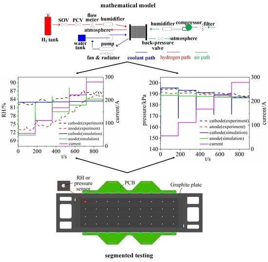
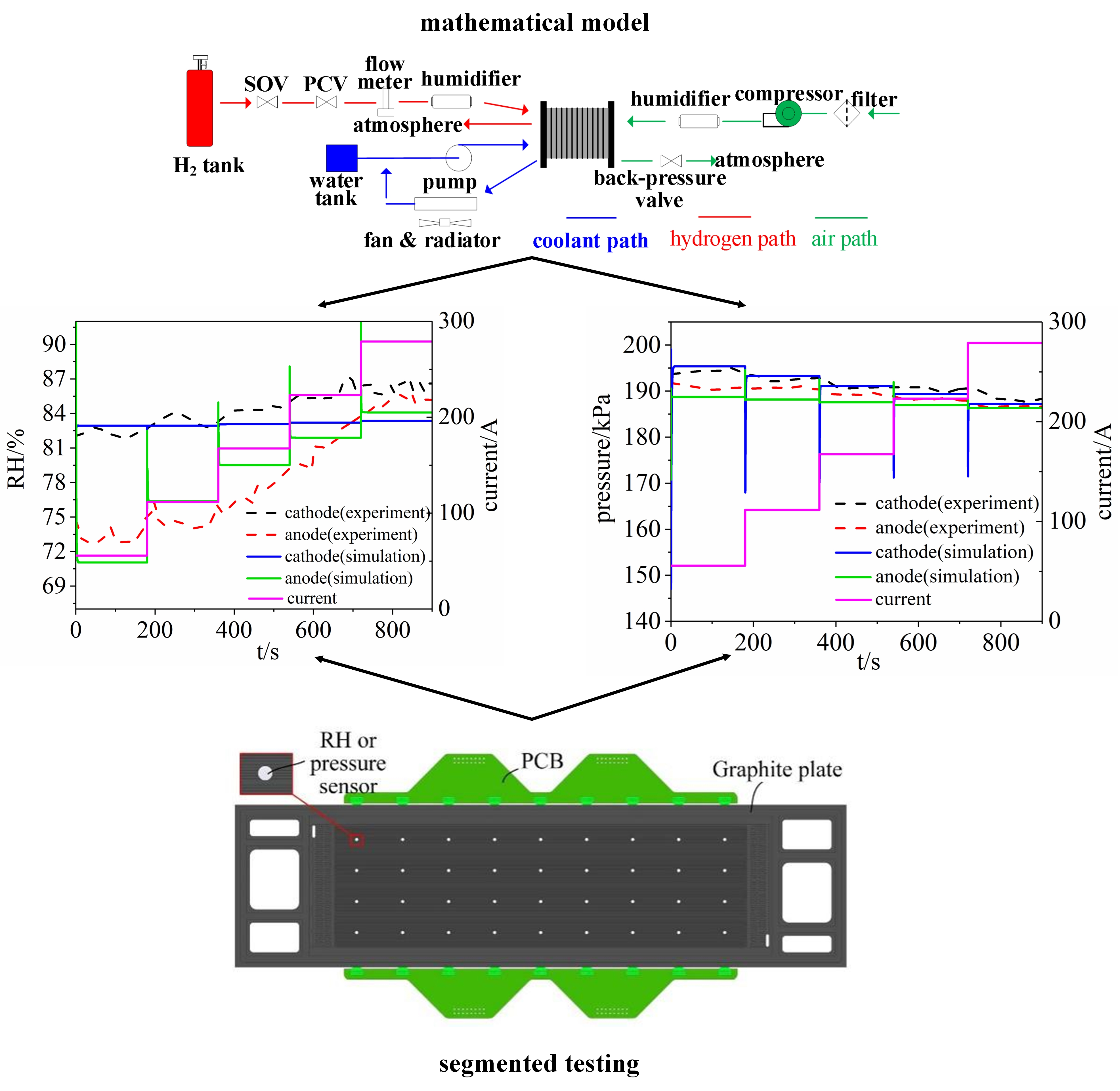
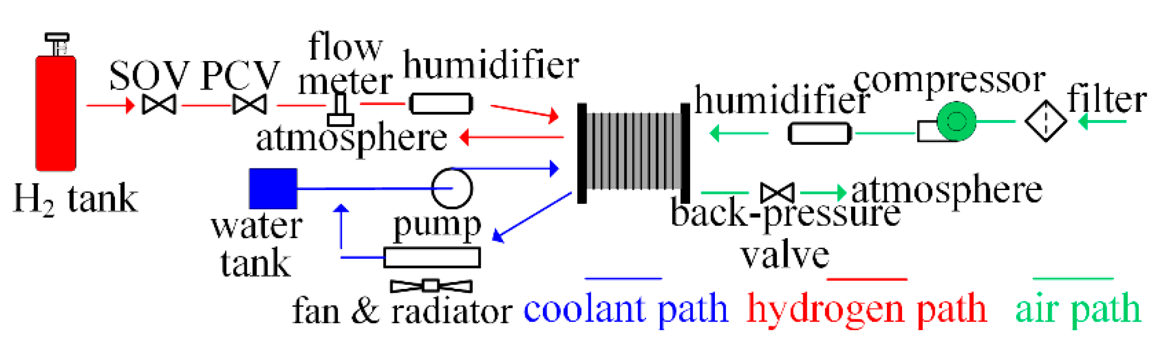
2. Mathematical Model and Experimental Platform

We claim the following assumptions made behind the model:

(a)

The gas dynamics follow the ideal gas equation of state (EoS).

(b)

Temperature, pressure and humidity distributed uniformly.

(c)

The stack operated well during the calculating period, local clogging, flooding and their influence on the stack state were not considered in this paper.

(d)

The water management was not considered in the model of water dynamics.

2.1. Operational Voltage

A single cell is calculated in this paper, which is consistent with the experimental method. The stack voltage, V_cell, can be described as Equation (1):

$$V_{cell}=V_{Nerst}-V_{act}-V_{conc}-I_{cell}{R}_{ohm}$$

(1)

where I_cell is the stack current, V_Nernst is the Nernst voltage, V_act is the activation overvoltage loss, V_conc is the concentration overvoltage loss, and R_ohm is the ohmic resistance.

The value of V_Nernst can be calculated by the Nernst equation, as shown in Equation (2):

$$V_{Nerst}=V_0+\frac{R{T}_{fc}}{2F}\ln (\frac{P_{H_2,an}}{P_0}\sqrt{\frac{P_{O_2,ca}}{P_0}})$$

(2)

where V₀ is the reversible cell potential at standard pressure, R = 8.31 J mol⁻¹ K⁻¹ and is the ideal gas constant, F = 96,483 C mol⁻¹ and is the Faraday constant, T_fc is the cell temperature, the average values of temperature from experimental results under different current were calculated and applied as known parameters in the simulation. P_H2,an and P_O2,ca are the partial pressures of hydrogen and oxygen gases in the anode and cathode channels, respectively, and P₀ = 100 kPa is the normalization coefficient.

The activation voltage loss, V_act, can be calculated using a Tafel equation:

$$V_{act}=\frac{R{T}_{fc}}{2\alpha F}\ln (\frac{I_{cell}+I_n}{I_0})$$

(3)

where α is the charge transfer coefficient, I_n is the internal current due to fuel crossover, and I₀ is the exchange current.

V_conc is the concentration voltage loss and can be calculated using Equation (4):

$$V_{conc}=\frac{R{T}_{fc}}{2F}\ln (1-\frac{I_{cell}+I_n}{I_1})$$

(4)

where I₁ is the limiting current at which the fuel is used at the maximum supply rate.

The cell ohmic resistance (R_ohm) consists of the resistance of the membrane, R_cell, and the conducting resistance, R₀ (see Equation (5)). R_cell is a function of water content and cell temperature, and it can be fitted using the experimental data from Peron et al. [7]:

$$\{\begin{array}{l}{R}_{Ohm}=R_{cell}+R_0\\ R_{cell}=\frac{L_m}{A_{cell}{\sigma }_m}\\ {\sigma }_m=f(\lambda )\end{array}$$

(5)

where L_m is membrane thickness, σ_m is membrane conductivity, A_cell is the active area of the cell, and λ is the water content in the PEM, the value of which can be obtained using Dutta et al.’s study [31].

2.2. Fluid Physics

The dynamic model for the cathode side includes air compressor, humidifier, supply and exhaust manifolds, cathode channel, and back valve; the anode side has similar structures except that hydrogen is discharged to the atmosphere directly. The mathematical models of different parts of the anode and cathode will be introduced below.

2.2.1. Gas Flow into the Stack

The hydrogen comes out from a high-pressure tank on the anode side and a flowmeter is used to regulate the fuel flow. On cathode side, air flow is controlled by the air compressor. To reduce calculations, the gas flow is simplified as Equation (6):

$${\dot{W}}_{in}\tau +W_{in}=W_{in,tg}$$

(6)

where W_in,tg is the target value for the mass flow of hydrogen and air, and τ is the time delay to reach the target value.

W_in,tg in anode and cathode sides can be calculated by as follows:

$$W_{in,catg}=0.0167N{\epsilon }_{ca}I{\rho }_{air}/60$$

(7)

$$W_{in,antg}=0.00697N{\epsilon }_{an}I{\rho }_{H_2}/60$$

(8)

where N is the cell number, ε_ca = 2.0 and ε_an = 1.3 are the stoichiometric ratios in cathode and anode, ρ_air and ρ_H2 are density of air and hydrogen.

2.2.2. Humidifier

The pressure difference between the humidifier and the supply manifold is negligible. The mole and mass fractions for the humidifier can be calculated as follows:

$$x_{vap,hum}=P_{sat}(T_{dew,hum})RH/P_{hum}$$

(9)

$$y_{gas,hum}=\frac{(1-x_{vap,hum})M_{gas}}{(1-x_{vap,hum})M_{gas}+x_{vap,hum}{M}_{H_{2}O}}$$

(10)

where x_vap,hum is the mole fraction of vapor at the output port of the humidifier, P_hum is the gas pressure in the humidifier, y_gas,hum is the mass fraction of air or hydrogen at the output port of the humidifier, T_dew,hum is the dew point of the humidified air, P_sat is the saturated vapor pressure, RH is the relative humidity in %, and M_gas and M_H2O are the molecular weights of reactant gases and water, respectively. We used Equation (11) to calculate the flow rate of mixed air and vapor in the humidifier:

$$W_{hum}=W_{cp}{y}_{gas,atm}/y_{gas,hum}$$

(11)

where W_cp is the rate of air flowing out from the air compressor, and y_gas,atm can be calculated as shown in Equation (10) using the atmospheric parameters.

2.2.3. Supply Manifolds

Assuming the temperature and pressure in the supply manifolds are uniform, the mass flow at the output port of the supply manifolds, W_sm,ca, can be expressed as follows (taking cathode side as example):

$$W_{sm}{}_{,ca}=k_{sm,ca}(P_{sm,ca}-P_{ca})$$

(12)

where k_sm,ca is the nozzle orifice coefficient of the supply manifolds, P_sm,ca and P_ca are the gas pressures in the supply manifolds and the cathode volume, respectively, and P_sm,ca is the supply manifold pressure, which can be expressed as follows:

$$\frac{d{P}_{sm,ca}}{dt}=\frac{R{T}_{cell}}{v_{sm,ca}{M}_{sm,ca}}(W_{hum,ca}-W_{sm,ca})$$

(13)

In Equation (13), v_sm,ca is the volume of the supply manifolds on the cathode side, M_sm,ca is the molar mass of the air mixture in the cathode manifolds, and W_hum is the mass flow rate of air through the humidifier. The molar mass of the mixed gas in the cathode manifolds M_sm,ca can be expressed as:

$$M_{sm,ca}=(1-x_{vap,hum})M_{air}+x_{vap,hum}{M}_{H_{2}O}$$

(14)

2.2.4. Cathode Channel

The cathode channel contains oxygen, nitrogen, water vapor, and liquid water. The mass balance equations are as follows:

$$\frac{d{m}_{O_2}}{dt}=W_{sm,ca}{y}_{O_2,sm}-\frac{I_{cell}}{4F}{M}_{O_2}-W_{ca}{y}_{O_2,ca}$$

(15)

$$\frac{d{m}_{N_2}}{dt}=W_{sm,ca}{y}_{N_2,sm}-W_{ca}{y}_{N_2,ca}$$

(16)

$$\frac{d{m}_{vap,ca}}{dt}=W_{sm,ca}{y}_{vap,sm}+\beta \frac{I_{cell}}{F}{M}_{H_{2}O}-N_{H_{2}O,diff}{A}_{cell}{M}_{H_{2}O}-W_{ca}{y}_{vap,ca}-\frac{d{m}_{phase}}{dt}-\theta \frac{d\lambda }{dt}{m}_{mem}$$

(17)

$$\frac{d{m}_{liq,ca}}{dt}=\frac{I_{cell}}{2F}{M}_{H_{2}O}+\frac{d{m}_{phase}}{dt}-W_{liq,ca}$$

(18)

The vapor change rate (Equation (17)) in cathode channel equals the algebraic sum of humid gas supplement, electro-osmotic drag water from anode to cathode, water diffusion from cathode to anode, flowing-out vapor, water condensation and membrane sorption (from left to right). Electrophoretic drag from cathode to anode due to concentration difference was neglected in this model because it is very small compared to other factors. Equation (18) shows the liquid water dynamics in cathode. The liquid water change rate is the algebraic sum of reaction product, water condensation and flowing-out liquid water. Actually, the influence of membrane water sorption usually can be neglected due to its slow change.

In these equations, m_O2, m_N2, m_vap,ca, and m_liq,ca are the respective masses of oxygen, nitrogen, water vapor, and liquid water in the cathode volume; y_O2,sm, y_N2,sm, y_vap,sm, y_O2,ca, y_N2,ca, and y_vap,ca are the respective mass fractions of oxygen, nitrogen, and water vapor in the supply manifolds and the cathode volume; W_ca is the mass flow rate of the mixed gas at the output port of the cathode volume; W_liq,ca is the liquid water mass flow at the output port of the cathode volume; m_phase is the water condensation in the cathode volume; M_O2 and M_H2O are the respective molar masses of oxygen and water vapor; N_H2O,diff is the water diffusion parameter which can be calculated according to ref [14] and n_d describes the number of water molecules dragged per H⁺ ion moved by electric field through the membrane, according to Ref. [5], n_d = 2.5λ/22.

The water content in the membrane λ is calculated by Equation (19). a is the water activity calculated by the mean value of relative humidity in the anode and cathode channels (Equation (20)) [14]. The water sorption equilibrium process in membrane usually costs more than 10⁵ s, so a delay module (1/(1 + 10⁵ s)) was applied in the model to simulate the slow process of water sorption.

$$\lambda =0.043+17.18a-39.85a^2+36a^3$$

(19)

$$a=(P_{ca}{x}_{vap,ca}/P_{sat,ca}+P_{an}{x}_{vap,an}/P_{sat,an})/2$$

(20)

In addition, the water droplet and slug formation process would affect the mass transport across GDL and flow channel, which in turn affects the PEMFC performance [12,32]. However, the model built in this paper is a lumped parameter model and it is limited to describe the local clogging phenomenon during mass transport, so it has to be assumed that the the gases and fluid water transport successfully inside the stack.

The pressure in the cathode volume, P_ca, can be calculated as follows:

$$P_{ca}=\frac{R{T}_{cell}}{v_{ca}}(\frac{m_{O_2}}{M_{O_2}}+\frac{m_{N_2}}{M_{N_2}}+\frac{m_{vap}}{M_{vap}})$$

(21)

The water condensation rate, m_phase, can be described as

$${\dot{m}}_{phase}=\{\begin{array}{l}\frac{k_c{v}_{ca}}{R{T}_{ca}}{x}_{vap,ca}(P_{ca}{x}_{vap,ca}-P_{sat})M_{H_{2}O} P_{ca}{x}_{vap,ca}\ge P_{sat}\\ k_e{m}_{liq,ca}(P_{ca}{x}_{vap,ca}-P_{sat}) P_{ca}{x}_{vap,ca}<P_{sat}\end{array}$$

(22)

where k_c is the steam condensation rate, k_e is the evaporation rate of liquid water, x_vap,ca is the molar fraction of water vapor in the cathode, and P_sat is the saturated water vapor pressure. The liquid water outflow from the cathode volume, W_liq,ca, can be expressed as follows:

$$W_{liq,ca}=\frac{k_{liq,ca}{m}_{liq,ca}}{m_{O_2}+m_{N_2}+m_{vap,ca}}{W}_{ca}$$

(23)

where k_liq,ca is a coefficient.

2.2.5. Anode Channel

The anode volume is comprised of hydrogen and water. The mass balance equations are as follows:

$$\frac{d{m}_{H_2}}{dt}=W_{sm,an}{y}_{H_2,sm}-\frac{I_{cell}}{2F}{M}_{H_2}-W_{an}{y}_{H_2,an}$$

(24)

$$\frac{d{m}_{vap,an}}{dt}=W_{sm,an}{y}_{vap,sm}-\beta \frac{I_{cell}}{F}{M}_{H_{2}O}+N_{H_{2}O,diff}{A}_{cell}{M}_{H_{2}O}-W_{an}{y}_{vap,an}-\frac{d{m}_{phase}}{dt}-(1-\theta )\frac{d\lambda }{dt}{m}_{mem}$$

(25)

$$\frac{d{m}_{liq,an}}{dt}=\frac{d{m}_{phase}}{dt}-W_{liq,an}$$

(26)

The pressure in the cathode volume, P_an, can be calculated as follows:

$$P_{an}=\frac{R{T}_{cell}}{v_{an}}(\frac{m_{H_2}}{M_{O_2}}+\frac{m_{vap}}{M_{vap}})$$

(27)

2.2.6. Cathode Exhaust Manifolds

The gas pressure in the exhaust manifolds of the cathode side, P_em,ca, can be expressed as follows:

$$\frac{d{P}_{em,ca}}{dt}=\frac{R{T}_{cell}}{v_{em,ca}{M}_{em,ca}}(W_{ca}-W_{em,ca})$$

(28)

where v_em,ca is the volume of the cathode exhaust manifolds, M_em,ca is the molar mass of the mixed gas, and W_em,ca is the mass flow rate at the output port of the manifolds. W_ca can be expressed as follows:

$$W_{ca}=k_{ca}(P_{ca}-P_{em,ca})$$

(29)

where k_ca is the nozzle orifice coefficient at the interface of the cathode volume and exhaust manifolds.

2.2.7. Anode Exhaust Manifolds

The gas pressure in the exhaust manifolds of the cathode side, P_em,an, can be expressed as follows:

$$\frac{d{P}_{em,an}}{dt}=\frac{R{T}_{cell}}{v_{em,an}{M}_{em,an}}(W_{an}-W_{em,an})$$

(30)

The two mass flows, W_em,an and W_an, can be expressed as follows:

$$W_{an}=k_{an}(P_{an}-P_{em,an})$$

(31)

$$W_{em,an}=k_{em,an}(P_{em,an}-P_{atm})$$

(32)

2.2.8. Back-Pressure Valve

The back-pressure valve is used to regulate the stack’s cathode inlet pressure. Laval nozzle flow theory is used to describe its mathematical features:

$$W_{em,ca}=s{\rho }_{em,ca}{(\frac{P_{atm}}{P_{em,ca}})}^{\frac{1}{k}}\sqrt{\frac{2k}{k-1}\frac{P_{em,ca}}{{\rho }_{em,ca}}[1-{(\frac{P_{atm}}{P_{em,ca}})}^{\frac{k-1}{k}}]}$$

(33)

where s is the opening area of the valve and is tested by experimental platform; ρ_em,ca is the gas density before the valve; and P_em,ca and P_atm are the pressures before and after the valve, respectively.

All the parameters used in the model are listed in

Table 1. Model parameters.

Parameters	Values	Parameters	Values
cathode channel volume, vca/cm3	5.088 (stack parameter)	cell internal current due to fuel crossover, In/A	3 (stack parameter)
cathode exhaust volume, vem,ca/cm3	0.15 (stack parameter)	cell nozzle orifice coefficient, kca/gPa−1s−1	3.71 × 10−5 (adjusted)
anode channel volume, van/cm3	2.387 (stack parameter)	cell nozzle orifice coefficient, ksm,ca/gPa−1s−1	2.199 × 10−5 (adjusted)
anode exhaust manifold volume, vem,an/cm3	0.07 (stack parameter)	cell nozzle orifice coefficient, kan/gPa−1s−1	1.51 × 10−6 (adjusted)
drag coefficient, nd	2.5λ/22 [5]	cell nozzle orifice coefficient, ksm,an/gPa−1s−1	2.28 × 10−6 (adjusted)
steam condensation rate, kc/s−1	100 [33]	cell nozzle orifice coefficient, kem,an/gPa−1s−1	5.08 × 10−8 (adjusted)
evaporation rate of liquid water, ke/atms−1	1 [34]	membrane thickness, lm/μm	25 (stack parameter)
liquid water coefficient, kliq/s−1	100 (ajusted)	effective area of each cell, Acell/cm2	186 (stack parameter)
cell exchange current, I0/A	0.0008 (stack parameter)	cell contact resistance, R0/mΩ	1 (stack parameter)
reversible cell potential at standard pressure, V0/V	1.229 (stack parameter)	cell limiting current, I1/A	320 (stack parameter)

.

2.3. Segmented Cell Testing Experiment to Verify the Model

A segmented cell testing experiment to test the pressure and humidity distribution on bipolar plates was conducted and is shown in Figure 2. In this study, each plate (graphite plate) was divided into 36 zones, and in each zone, humidity and pressure sensors were installed to measure the humidity and pressure distribution for different current densities. The relative humidity (RH) measurement is based on sensitive change of polymer material capacitance under different humidity, while the pressure testing is based on the resistance change of pressure sensitive resistor. The test errors of RH and pressure are 1.5% and ±4.0 kPa respectively. PCB (print circuit board) is used to collect signals from sensors and communicate with the upper computer with Labview. To reduce the influence of so many sensors, only one field was tested in each experiment.

2.4. Calculations and Experimental Conditions

In the simulation and experimental processes, the inlet pressures were set at 203 kPa and 201 kPa at the anode and cathode sides, respectively, with relative humidity (RH) values of 100% and 50%. The hydrogen and air were in co-flow mode. The requisite fuel and oxidant flows were calculated using stack current and stoichiometric ratios. The stoichiometric ratios were 1.3 and 2.0, respectively, consistent with the experimental platform.

In the simulation process, a current of 55.8 A was selected as the initial condition for the calculations, then the load current was increased with time, as shown in

Table 2. Current density used in the simulation process.

Time (s)	0–20	20–40	40–60	60–80	80–100
Current (A)	55.8	111.6	167.4	223.2	279

, and the dynamic process inside the stack was calculated.

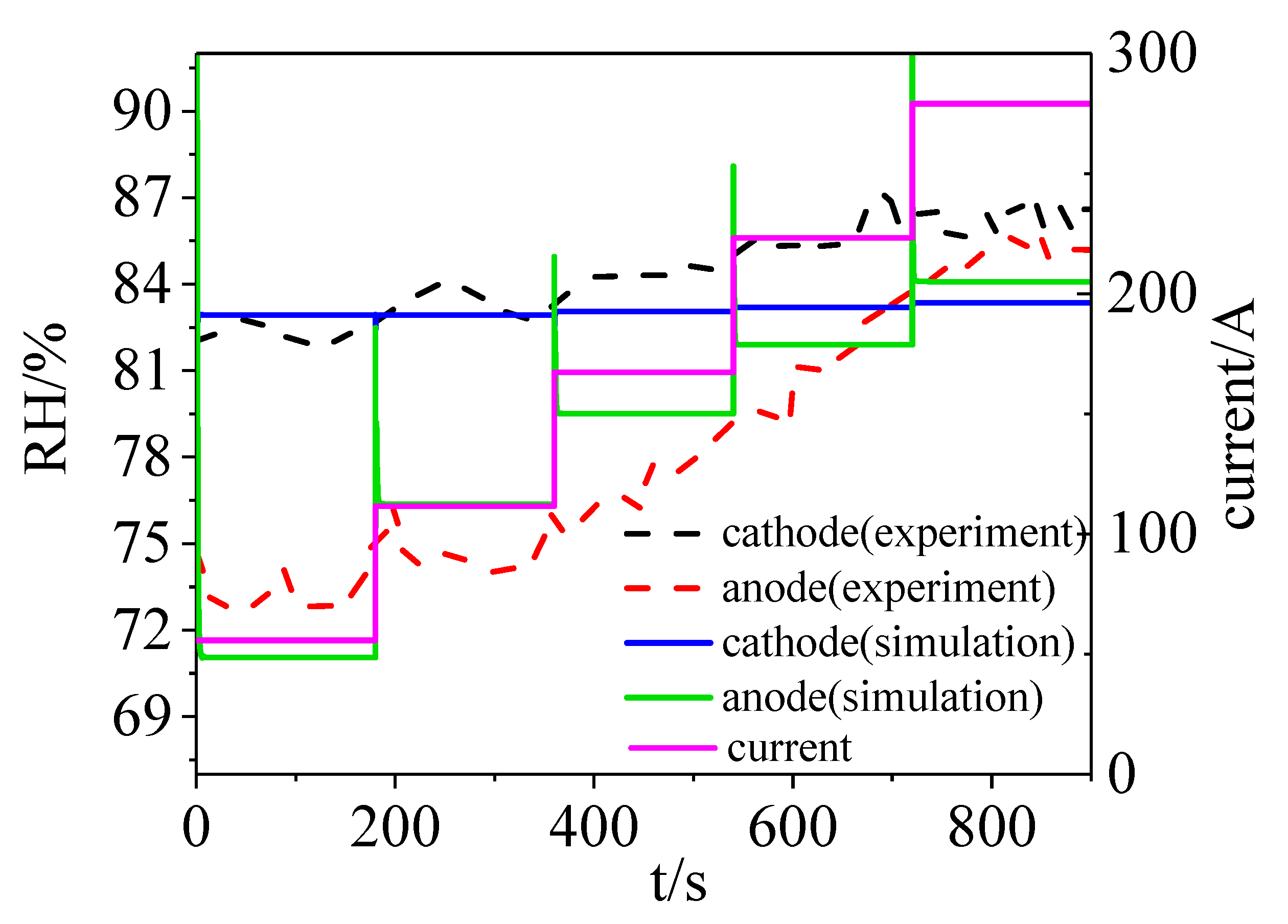
3. Results and Model Verification

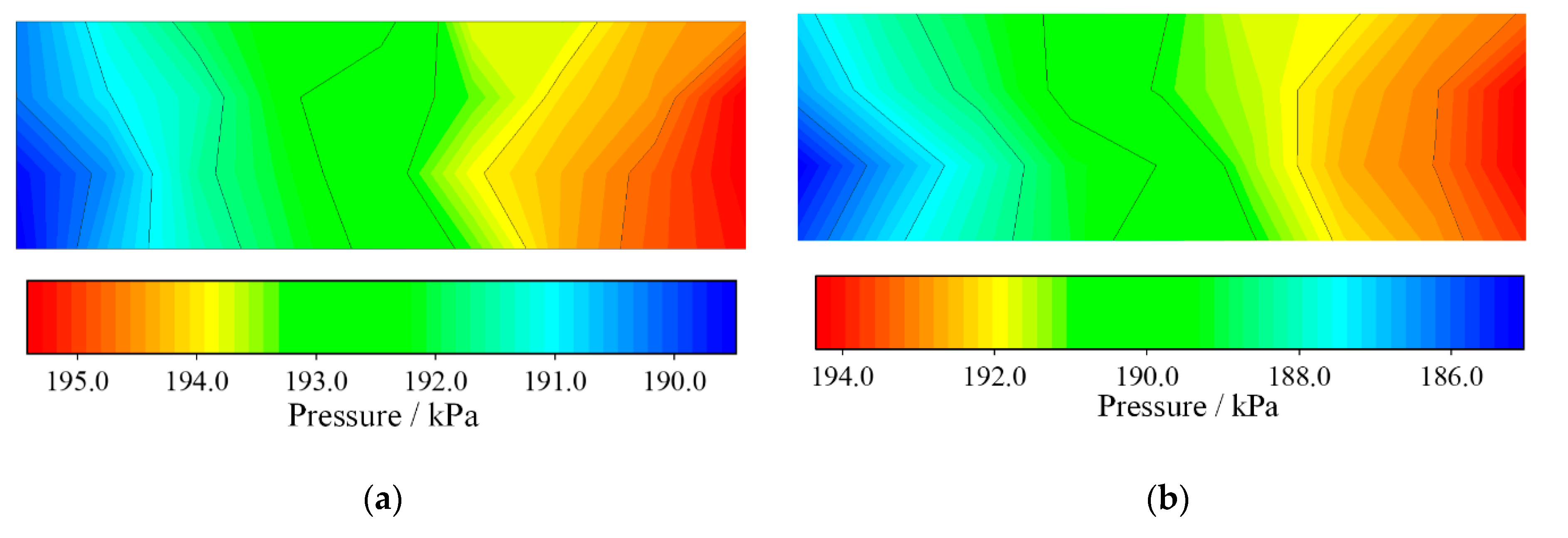
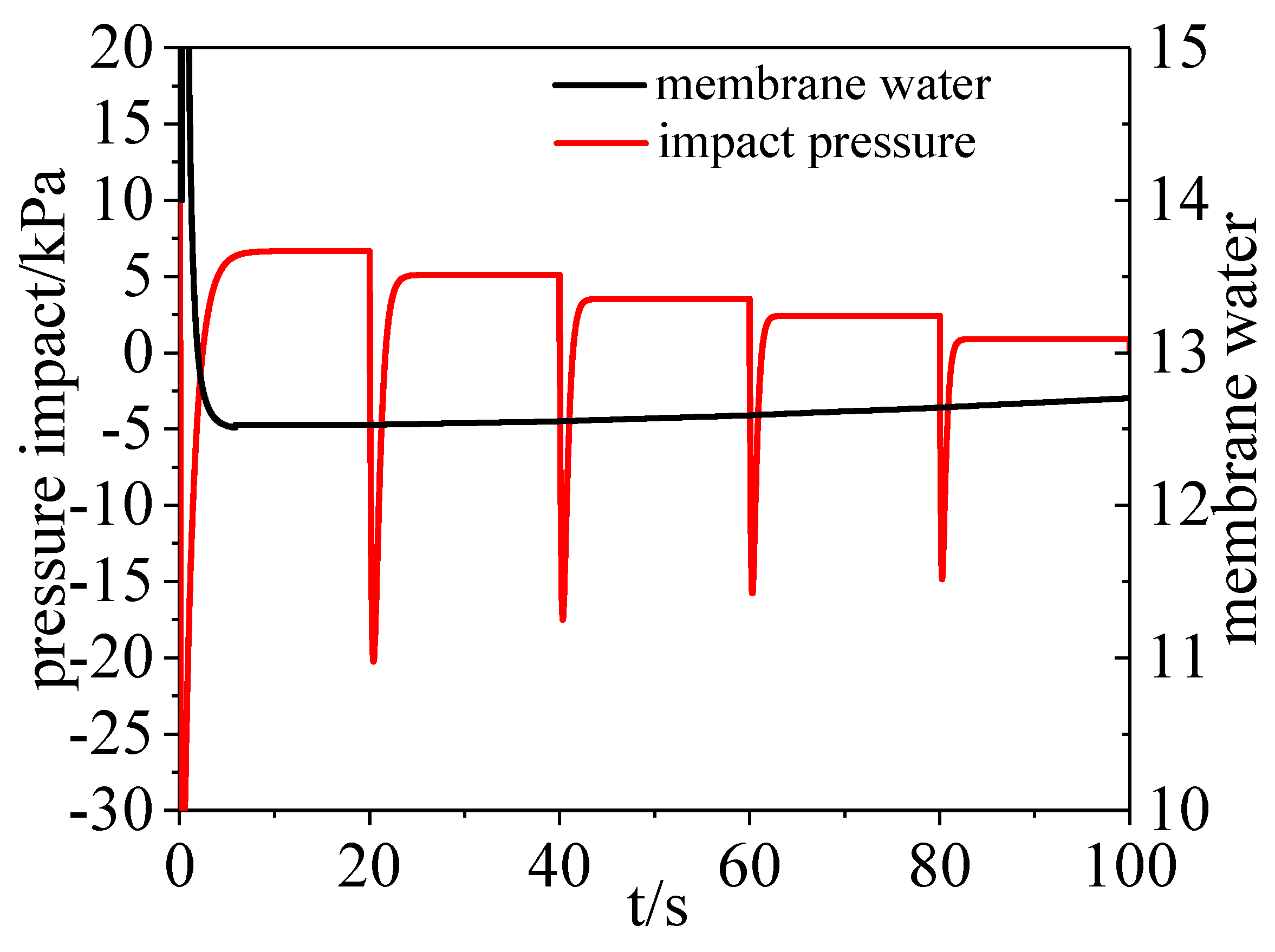
3.1. Pressure Dynamics

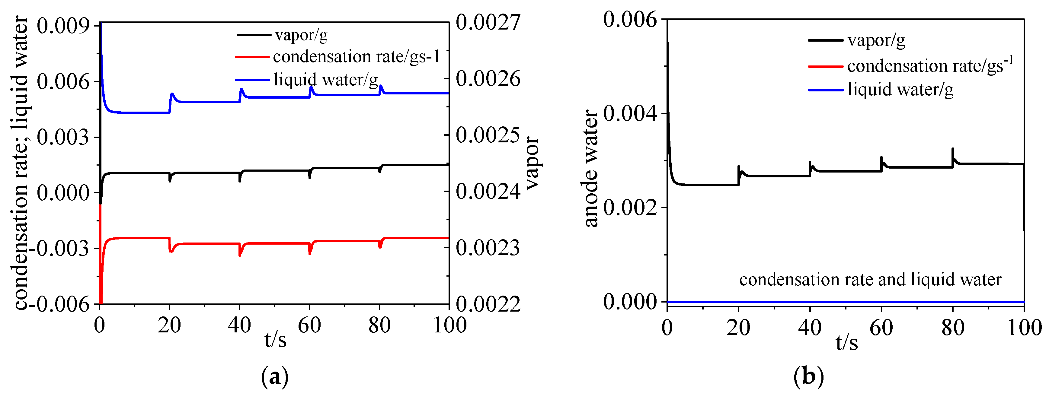
The pressure dynamics in the supply manifolds, channel and exhaust manifolds can be obtained, as can be seen in Figure 3. The pressure fluctuated when load current changed with time, and it shows obvious declines in the pressure from the supply manifolds, to the channel, to the exhaust manifolds. The pressure inside the channel and exhaust manifold declined gradually as the load current rose, because of the increasing oxygen consumption and the action of the back-pressure valve. On the anode side, the pressure in the channel and exhaust manifolds also decreased with time.

The pressure distribution from the segmented cell platform is shown in Figure 4 (in the interest of space, only the cathode channel pressure is shown as an example). It can be seen that the pressure declined gradually from stack inlet (right) to stack outlet (left) which consistent with the simulation results.

The average pressure from the experiment inside the channel was calculated and compared with the simulation results (the current was increased every 3 min considering the operating condition of the stack), as shown in Figure 5. It can be seen that the experimental pressure and calculated pressure showed the same trend with current. In addition, the average relative error of calculated results is less than 5%, which verifies the simulation model built in this study to some extent.

3.2. Water Dynamics

Water content and its transition between states in the channel are important indicators for monitoring states and diagnosing faults in a PEMFC. Values for vapor, liquid water, and the water condensation are shown in Figure 6. On the cathode side, when the load current increased, the amount of vapor and liquid water increased gradually with current. Water condensation rate fluctuated only slightly. On the anode side, vapor increased with time slightly under the multi-process of water diffusion and electro-osmotic drag, while water condensation and liquid water seldom existed.

The RH distribution under different load currents was obtained by the experimental method, the results of which are shown in Figure 7. RH clearly increased from stack inlet to stack outlet, based on the field distribution data.

The average RH value was calculated from the experimental data, and Figure 8 compares the experimental and simulation results (the RH results from the simulation were calculated using Equation (9)). It can be seen that RH in cathode channel and anode channel both increased with current under the conditions set in this paper.

With the simulation model above, we were able to obtain the membrane water and pressure impact on the MEA (i.e., the difference between the cathode and anode pressure), which we could not measure experimentally. Water content in the membrane increased very slowly with load current according to the calculation results shown in Figure 9, because the water sorption process in the membrane usually cost more than 10⁵ s. With load variation, the pressure difference between the cathode and anode channel pressure, and hence the pressure impact on the MEA, also fluctuated. The impact was particularly large, in the order of kPa.

Based on the above results, it can be concluded that the PEMFC underwent obvious state change inside the stack when the load current varied over time, potentially leading to unpredictable faults and even adversely influencing the stack’s lifespan. In the aspect of pressure dynamics, the anode and cathode pressure decreased with time because more oxygen and hydrogen were consumed when a larger current was needed. On the cathode side, the back-pressure valve connected to the atmosphere usually had a bigger opening when a larger load occurs, causing the channel pressure to drop again. Changes in anode and cathode pressure meant the MEA was subjected to pressure fluctuations, and steep pressure increases threatened the MEA’s structure and materials.

Water content is also a very important indicator for evaluating a stack’s operating state. The water dynamics in the flow channel comprise a complicated balancing process involving reactive synthesis, bidirectional diffusion, phase transition, and so on. Under the conditions described in this paper, the amount of water vapor and the water condensation rate in the cathode channel changed slightly with the load current, while the amount of liquid water gradually increased. On the anode side, water vapor increased with load, while there were nearly no liquid water and water condensation existing.

4. Discussion

As described above, we were able to verify the model’s reliability to some extent, and we found that the stack’s steady state was disrupted with load fluctuation. Based on these findings, we used the model to study how the load change magnitude and the time interval of load variation affected the stack.

4.1. Role of Load Change Magnitude

A current of 55.8 A was chosen as the initial value. It was then increased to 111.6 A, 167.4 A, 223.2 A, and 279 A over a period of 10 s. Figure 10 presents a curve showing the relationship between state change and current change magnitude. It can be seen from Figure 10a that as the current was increased from 55.8 A, the magnitude of the pressure impact and output voltage increased almost linearly, while membrane water change only increased slightly. Figure 10b shows that the RH change in the cathode and anode channels also increased with current change, and the increasing rate of anode was bigger in this paper.

4.2. Role of Time Interval of Load Change

In actual operation, a PEMFC’s operational mode changes over time, usually at very short intervals, which leads to sharp state changes in the PEMFC. According to our calculated results, the trends in pressure, RH in cathode and anode at different time intervals were similar when the time was greater than 5 s. However, when the interval was reduced to 1 s, the PEMFC struggled to maintain a steady state (Figure 11b). It can also be concluded from Figure 11 that a shorter time interval altered the normal trend of the state parameters, resulting in even greater stress on the MEA.

5. Conclusions

The following conclusions can be drawn:

• A complete model involving a PEMFC stack and its accessories was built in this paper, and it was verified to some extent by a segmented testing experiment. This model can be used to simulate the dynamic state inside the stack.
• The pressure in the channels, and exhaust manifolds declined with increasing current. The transient pressure difference between the cathode and anode sides had a huge impact on the MEA.
• On the cathode side, the vapor and liquid water increased when the load current increased. On the anode side, water vapor increased with time while there was hardly any liquid water and water condensation existing in the channel.
• Changes in the outside load definitely influenced the stack’s stability in terms of pressure, water, and voltage. When the magnitude of the current change increased, the stack state underwent greater fluctuation. If the load varied in a short enough time, the stack components and physical processes could not reach equilibrium.

References

1. Aaldering, L.J.; Song, C.H. Tracing the technological development trajectory in post-lithium-ion battery technologies: A patent-based approach. J. Clean. Prod. 2019, 241, 1–18. [Google Scholar] [CrossRef]
2. U.S. Department of Energy. Available online: https://www.energy.gov/eere/fuelcells/hydrogen-and-fuel-cells-annual-progress-reports (accessed on 1 April 2019).
3. China Nengyuan.com. Available online: http://www.china-nengyuan.com/news/141562.html (accessed on 2 July 2019).
4. Bao, C.; Ouyang, M.; Yi, B. Modeling and control of air stream and hydrogen flow with recirculation in a PEM fuel cell system—I. control-oriented modeling. Int. J. Hydrog. Energy 2006, 31, 1879–1896. [Google Scholar] [CrossRef]
5. Springe, T.E.; Zawodzinski, T.; Gottesfeld, A.S. Polymer electrolyte fuel cell model. J. Electrochem. Soc. 1991, 138, 2334–2342. [Google Scholar] [CrossRef]
6. Xu, L.; Fang, C.; Hu, J. Parameter extraction and uncertainty analysis of a proton exchange membrane fuel cell system based on Monte Carlo simulation. Int. J. Hydrog. Energy 2017, 42, 2309–2326. [Google Scholar] [CrossRef]
7. Peron, J.; Mani, A.; Zhao, X. Properties of Nafion® NR-211 membranes for PEMFCs. J. Membr. Sci. 2010, 356, 44–51. [Google Scholar] [CrossRef]
8. Deevanhxay, P.; Sasabe, T.; Tsushima, S.; Hirai, S. In situ diagnostic of liquid water distribution in cathode catalyst layer in an operating PEMFC by high-resolution soft X-ray radiography. Electrochem. Commun. 2012, 22, 33–36. [Google Scholar] [CrossRef]
9. Deevanhxay, P.; Tsushima, S.; Hirai, S. Investigation on the effect of microstructure of proton exchange membrane fuel cell porous layers on liquid water behavior by soft X-ray radiography. J. Power Sources 2011, 196, 8197–8206. [Google Scholar]
10. Suzuki, T.; Tabuchi, Y.; Tsushima, S. Measurement of water content distribution in catalyst coated membranes under water permeation conditions by magnetic resonance imaging. Int. J. Hydrog. Energy 2011, 36, 5479–5486. [Google Scholar] [CrossRef]
11. Jay, B. Fan the flame with water: Current ignition, front propagation and multiple steady states in polymer electrolyte membrane fuel cells. AICHE J. 2009, 55, 3034–3040. [Google Scholar]
12. Erin, K.; Tamara, W.; Yannis, K.; Jay, B. Drops, slugs, and flooding in polymer electrolyte membrane fuel cells. AICHE J. 2008, 54, 1313–1320. [Google Scholar]
13. Luna, J.; Jemei, S.; Yousfifi-Steiner, N.; Husar, A.; Serra, M. Nonlinear predictive control for durability enhancement and efficiency improvement in a fuel cell power system. J. Power Sources 2016, 328, 250–261. [Google Scholar] [CrossRef] [Green Version]
14. Barbir, F. PEM Fuel Cell: Theory and Practice, 2nd ed.; Elsevier Press: Amsterdam, The Netherlands, 2012; p. 25. [Google Scholar]
15. Fang, C. Fuel Cell Engine Control Based on Reduced Dimension Model. Ph.D. Thesis, Tsinghua University, Beijing, China, 2017. [Google Scholar]
16. Hua, J.; Li, J.; Ouyang, M. Proton exchange membrane fuel cell system diagnosis based on the multivariate statistical method. Int. J. Hydrog. Energy 2011, 36, 9896–9905. [Google Scholar] [CrossRef]
17. Hong, P.; Xu, L.; Li, J. Modeling and analysis of internal water transfer behavior of PEM fuel cell of large surface area. Int. J. Hydrog. Energy 2017, 42, 18540–18550. [Google Scholar] [CrossRef]
18. Sui, P.; Zhu, X.; Djilali, N. Modeling of PEM fuel cell catalyst layers: Status and outlook. Electrochem. Energy Rev. 2019, 2, 428–466. [Google Scholar] [CrossRef]
19. Tian, N.; Lu, B.; Yang, X. Rational design and synthesis of low-temperature fuel cell electrocatalysts. Electrochem. Energy Rev. 2018, 1, 54–83. [Google Scholar] [CrossRef] [Green Version]
20. Xu, L.; Fang, C.; Hu, J. Self-humidification of a polymer electrolyte membrane fuel cell system with cathodic exhaust gas recirculation. J. Electrochem. Energy Convers. Storage 2018, 15, 1–18. [Google Scholar] [CrossRef]
21. Hong, P.; Xu, L.; Li, J. Modeling of membrane electrode assembly of PEM fuel cell to analyze voltage losses inside. Energy 2017, 139, 277–288. [Google Scholar] [CrossRef]
22. Xu, L.; Fang, C.; Li, J. Nonlinear dynamic mechanism modeling of a polymer electrolyte membrane fuel cell with dead-ended anode considering mass transport and actuator properties. Appl. Energy 2018, 230, 106–121. [Google Scholar] [CrossRef]
23. Zhang, Q.; Xu, L.; Li, J. Performance prediction of proton exchange membrane fuel cell engine thermal management system using 1D and 3D integrating numerical simulation. Int. J. Hydrog. Energy 2018, 43, 1736–1748. [Google Scholar] [CrossRef]
24. Pasaogullari, U.; Mukherjee, P.; Wang, C.; Chen, K. Anisotropie heat and water transport in a PEFC cathode gas diffusion layer. J. Electrochem. Soc. 2007, 154, B823. [Google Scholar] [CrossRef]
25. Vladimir, G.; Adin, M. A critical overview of computational fluid dynamics multiphase models for proton exchange membrane fuel cells. SIAM J. Appl. Math 2009, 70, 410–454. [Google Scholar]
26. Lin, R.; Lin, X.; Weng, Y. Evolution of thermal drifting during and after cold start of proton exchange membrane fuel cell by segmented cell technology. Int. J. Hydrog. Energy 2015, 40, 7370–7381. [Google Scholar] [CrossRef]
27. Lin, R.; Weng, Y.; Li, Y. Internal behavior of segmented fuel cell during cold start. Int. J. Hydrog. Energy 2014, 39, 16025–16035. [Google Scholar] [CrossRef]
28. Pei, H.; Liu, Z.; Zhang, H. In situ measurement of temperature distribution in proton exchange membrane fuel cell I a hydrogeneair stack. J. Power Sources 2013, 227, 72–79. [Google Scholar] [CrossRef]
29. Lin, R.; Cui, X.; Shan, J. Investigating the effect of start-up and shut-down cycles on the performance of the proton exchange membrane fuel cell by segmented cell technology. Int. J. Hydrog. Energy 2015, 40, 14952–14962. [Google Scholar] [CrossRef]
30. Lin, R.; Xiong, F.; Tang, W. Investigation of dynamic driving cycle effect on the degradation of roton exchange membrane fuel cell by segmented cell technology. J. Power Sources 2014, 260, 150–158. [Google Scholar] [CrossRef]
31. Dutta, S.; Shimpalee, S.; Zee, J. Numerical prediction of mass-exchange between cathode and anode channels in a PEM fuel cell. Int. J. Heat Mass Transf. 2001, 44, 2029–2042. [Google Scholar] [CrossRef]
32. May, C.; Ioannis, K.; Jay, B. Water slug formation and motion in gas flow channels: The effects of geometry, surface wettability, and gravity. Langmuir 2013, 29, 9918–9934. [Google Scholar]
33. Wensheng, H.; Jung, S.; Trung, N. Two-phase flow model of the cathode of PEM fuel cells using interdigitated flow fields. AIChE J. 2000, 46, 2053–2060. [Google Scholar]
34. Dilip, N.; Trung, N. A two-dimensional, two-phase, multicomponent, transient model for the cathode of a proton exchange membrane fuel cell using conventional gas distributors. J. Electrochem. Soc. 2001, 48, 1324–1335. [Google Scholar]
Figure 1. Schematic of a proton exchange membrane fuel cell (PEMFC) system.
Energies 13 03596 g001
Figure 2. Segmented testing schematic on a bipolar plate. (a) segmented testing platform. (b) segmented zones on a bipolar plate.
Energies 13 03596 g002
Figure 3. Pressure dynamics in the channel, according to calculations: (a) cathode, (b) anode.
Energies 13 03596 g003
Figure 4. Pressure dynamics in the cathode channel, from the experiment: (a) under current of 111.6 A, (b) under current of 167.4 A.
Energies 13 03596 g004
Figure 5. Comparison of experimental and simulation results for pressure.
Energies 13 03596 g005
Figure 6. Calculated values for the water dynamics in the channel: (a) cathode channel water, (b) anode channel water.
Energies 13 03596 g006
Figure 7. Experimental results for relative humidity (RH) distribution in the anode channel: (a) under current of 55.8 A, (b) under current of 167.4 A.
Energies 13 03596 g007
Figure 8. Comparison of experimental and simulation results for RH in channel.
Energies 13 03596 g008
Figure 9. Water content in the membrane and pressure impact on membrane electrode assembly (MEA), from simulation results.
Energies 13 03596 g009
Figure 10. Changes in PEMFC state with current changes. (a) pressure impact, membrane water and output voltage (b) RH.
Energies 13 03596 g010
Figure 11. RH and pressure impact on the MEA at different time intervals: (a) at interval of 10 s, (b) at interval of 1 s, (c) at interval of 0.2 s.
Energies 13 03596 g011aEnergies 13 03596 g011b