Abstract
The main objective of this study is to calculate and determine design parameters for a novel wire cloth micro heat exchanger. Wire cloth micro heat exchangers offer a range of promising applications in the chemical industry, plastics technology, the recycling industry and energy technology. We derived correlations to calculate the heat transfer rate, pressure drop and temperature distributions through the woven structure in order to design wire cloth heat exchangers for different applications. Computational Fluid Dynamics (CFD) simulations have been carried out to determine correlations for the dimensionless Euler and Nusselt numbers. Based on these correlations, we have developed a simplified model in which the correlations can be used to calculate temperature distributions and heat exchanger performance. This allows a wire cloth micro heat exchanger to be virtually designed for different applications.
1. Introduction
In order to tackle problems in energy management, improvements in the efficiency of existing systems are needed. In this context, the miniaturization of heat exchangers has been a constant area of research for decades [1,2]. A limiting factor in many configurations, whether parallel-, counter- or cross-flow, is the heat transfer from the gas-phase to the solid medium. A metallic wire-screen/tubing structure, as shown schematically in Figure 1, can be used to reduce this limitation by increasing the volume-specific heat transfer surface area and magnifying the contact area between gas-phase and heat exchanger [3,4].
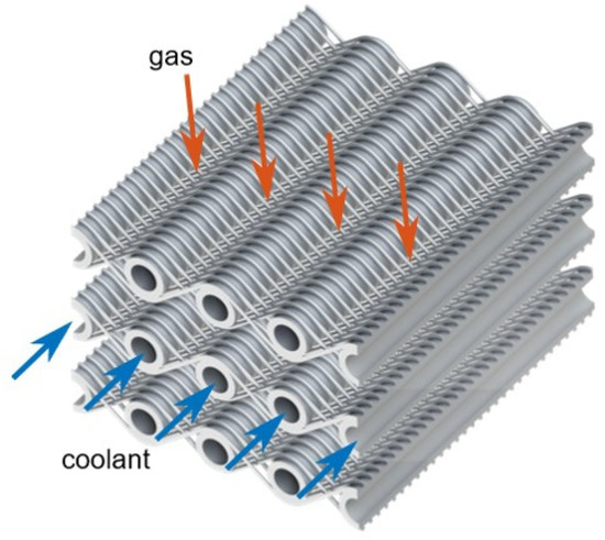
Figure 1.
Illustration of a woven cloth micro heat exchanger featuring a wire-screen/tubing structure, with coolant flow through tubes in blue and cross-flow of gas through the wire-screen in red.
Wire screens are regular structures, consisting of small diameter wires which are woven in two orthogonal directions in a plane, similar to woven textile materials. There is a range of different types of weaves that are suited for heat exchange applications. A modification of the standard linen weave, employed in this context, consists of replacing the weft wire with small diameter tubes. The resulting cross-flow heat exchanger, shown in Figure 1, is highly versatile and provides a high volume-specific heat transfer surface area. It can be used in the chemical industry, by applying a catalyst coat on the surface of the screen, or in energy storage applications in combination with phase change materials. The concept of the wire-screen heat exchanger was introduced and experimentally investigated in [5,6,7]. These studies with multilayer meshes in a rectangular channel and with variations in the wire structure suffered from poor thermal contact between the tubes and the wires. The resulting heat transfer coefficients were significantly lower than those of comparable systems. We refer to an improved and patented concept that increases the thermal contact, as presented in [8]. Experimental and numerical investigations of these systems were conducted by Martens and Fugmann et al. [9,10,11], with an extension to different wire-on-tube structures by the latter authors. The improvements resulted in increased heat transfer coefficients which are in the upper range of comparable compact heat exchangers.
Woven wire mesh structures allow a broad variety of combinations of geometric dimensions and shapes. In conjunction with the properties of the working fluids used, they offer numerous possibilities for optimizing heat exchanger cost and performance for a wide range of operating conditions. Due to the large number of influencing parameters, research into the thermal transmission potential and the development of design criteria on a purely experimental basis is not expedient [12,13,14]. For this reason, this article presents a numerical approach to characterize and calculate the heat transfer across wire cloth heat exchangers of the type shown in Figure 1. For an efficient design of the heat exchanger, the transmitted heat flow, the pressure drop and the temperature profiles along the tubes and along the wires are of particular interest.
In the first step, the gas-side heat transfer coefficient is determined numerically using CFD simulations. With this, the heat flow as well as the average gas and coolant temperatures can be determined by a P-NTU approach. The temperature profile in tube direction, which is particularly relevant for applications in chemical reaction engineering, is calculated by an effective 1-D model (EM). The maximum temperature along the wire can be determined analytically by considering the wires to be connected to the tube as fins [15]. For all calculations, water is used as coolant and air as gas with temperature-dependent material values. In the following, the geometry and the relevant parameters of the heat exchanger are presented.
2. Materials and Methods
2.1. Geometric Parameters
Following the approach of Balzer [8] and assuming a common inlet and outlet for the coolant tubes, the heat exchanger configuration shown in Figure 2a with the length dimensions , and , is considered. The total volume of the heat exchanger is given by
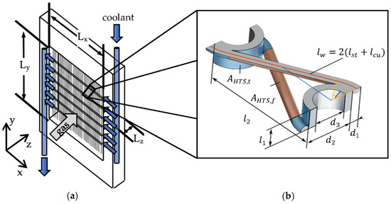
Figure 2.
(a) Schematic view of the entire woven wire heat exchanger with common manifold inlet and outlet for the coolant tubes colored in blue. The relevant length dimensions are shown with the axes of the heat exchanger tubes pointing in the x-direction. (b) Characteristic symmetric/periodic (in the x- and y-directions) section of the woven heat exchanger with relevant geometric variables. The gas-side heat transfer surface area can be separated in the tube and connected wire and fin .
The wires are combined with the tubes in a weaving process comparable to that known from textiles. Solder is added in order to stabilize the structure and improve the thermal contact between wires and tubes. Wire diameters can range from 100 µm to 1 mm. The outer diameter of the tubes can be significantly less than 2 mm and with small wall thicknesses (in the range of 100 µm) while providing high-pressure resistance [16].
The characteristic geometric parameters of the wire-screen/tubing structure are shown in a representative section of the heat exchanger in Figure 2b. Whereby denotes the distance between the centers of two wires in the y-direction, the distance between the tube centers in the x-direction and the inner tube diameter. The total number of tubes and wires is therefore given by
A dimensionless diameter
dimensionless warp wire pitch
and dimensionless weft tube pitch
are used to characterize geometric variations of the heat exchanger.
In Figure 2b, denotes the entire length of the wire within the periodic section and is composed of a curved part attached to the tube and a straight section . The latter can be calculated as follows:
where the tangential angle
describes half the angle over which a tube and a wire are in contact. In other words, it describes the angular range over which the wire bends around a tube. Based on geometrical considerations, the overall gas-side heat transfer surface area , composed of the tube surface area with connected wire area and the wire fin surface area can be calculated from Equations (9)–(11):
Additional geometric parameters are the gas-side specific surface area of the solid in relation to the total heat exchanger volume and the gas fraction , which are defined as:
With the help of additional dimensionless parameters, it is possible to quickly investigate the behavior of the system. For the characterization of heat exchangers, gas-side pressure loss and heat transfer rate are of interest under given operating conditions. The dependencies are governed by a set of geometry parameters, as well as Reynolds, Euler and Nusselt numbers. Here, the Reynolds number is based on the undisturbed inflow velocity , gas-phase density and viscosity , and the specific surface area of the mesh structure
The Euler number is defined by the ratio of the gas-phase static pressure drop across the heat exchanger and the dynamic pressure of the undisturbed flow
The Nusselt number of the gas-side surface heat transfer is defined as
where by denotes the gas-side heat transfer coefficient, is the thermal conductivity of the gas and again serves as characteristic length.
2.2. Heat Transfer Paths and Mechanisms
The overall heat transfer through the woven wire mesh heat exchanger can be separated into five contributions:
- Heat transfer between the coolant and the tubes;
- Heat conduction in the tube walls;
- Heat conduction in the wires;
- Heat transfer between the tubes and curved wire sections and the gas;
- Heat transfer between the straight wire sections as a fin and the gas.
The heat transfer between the coolant and the tube can be described using correlations for laminar pipe flow from literature [17]. Heat conduction in the solid phase can be described using Fourier’s law. Heat transfer between the gas and the heat exchanger’s outer surface, on the other hand, must be derived from numerical simulations.
The logarithmic temperature difference as driving force for the heat transfer is defined as
with the gas outflow temperature , the inflow temperature and the mean temperature of the heat transfer surface .
In order to reduce the complexity of the problem, the concept of fin efficiency can be applied, as described in [18]. Accordingly, the straight part of the wire is assumed to be a fin with a rectangular profile and the thickness . A mean heat transfer coefficient between the gas and solid phase, which does not vary significantly along the surface, is defined and the temperature profile in the fin is given by
with
where is the fin temperature and is the distance on the fin from the base of the fin referred to as fin coordinate, with the length of the straight wire part representing the fin length. The ambient temperature is approximated by the gas inlet temperature . Considering low thermal resistance for the heat transfer through the tube, the temperature at the base of the fin is approximately the coolant temperature . With this assumption we obtain Equation (20) for the maximum temperature rise along the wire for .
Taking the fin efficiency into account, the gas-side heat transfer is described by Equation (21).
whereby the fin efficiency , given by
is a function of .
2.3. 3D-Computational Fluid Dynamics Simulation (CFD)
The aim of the numerical model presented here is the numerical determination of the heat transfer coefficient for a large variation of the heat exchanger’s geometric parameters. The governing equations in the gas flow and solid region are solved using OpenFoam®, while the liquid flow in the tubes can be modeled analytically assuming constant coolant temperature () and using Nu-correlations from the literature. For the gas flow the following assumptions are made:
- Gas density is constant and heat generation due to frictional forces is negligible, due to low gas-phase velocities (Mach number << 1);
- All material properties are calculated for a constant temperature;
- Natural convection is negligible compared to the imposed forced convective flow;
- Heat transfer into the environment and radiative heat transfer is negligible.
The gas-phase governing equations to be solved based on the prescribed assumptions are Equations (23)–(25).
where , , ,, and denote velocity vector, density, pressure, shear stress tensor, the transferred heat flux density and temperature in the gas-phase and and represent the dynamic viscosity and specific heat capacity of the gas. In the area of the fabric, specific Reynolds numbers below 1000 occur at low flow velocities (up to approx. ) and therefore a laminar state around the fabric is expected.
In the solid phase, only a heat conduction equation has to be solved, i.e.,
with the thermal conductivity , the heat capacity and the density of the solid phase material.
Coupling between the fluid and solid phase domains is achieved via boundary conditions (BC) as illustrated in Figure 3. The applied boundary conditions are summarized in Table 1. A Neumann BC for the temperature field is applied on boundary faces (W) pertaining to both solid and fluid domains. The gradient is calculated by Equation (27) conservation of heat flux through the boundary face
with as the thermal conductivity of the gas and the solid and as the normal vector.
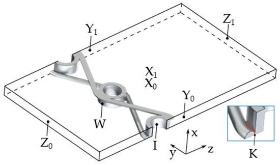
Figure 3.
Illustration of the computational domain and domain boundaries used for the Computational Fluid Dynamics (CFD) analysis of a periodic/symmetric section of the heat exchanger. The contact surface between tube and wire with thermal resistance K is enlarged.

Table 1.
Overview of the boundary conditions employed for the CFD analysis.
On the fluid side default (nonslip) wall BCs are employed. Temperature and velocity at the inlet (located at ) as well as the pressure at the outlet (located at ) are fixed, while zero gradients in the respective variables are set at opposing sides of the flow field. In tube direction (x-direction) symmetry conditions are imposed at the boundaries of the simulation domain, i.e., at . In warp-wire direction (y-direction) the geometry is mirrored, and cyclic BCs are applied at , which allows to capture unsteady flow behavior like vortex shedding. The temperature gradients in the tubes are expected to be small compared to the other heat transport mechanisms. The velocity field is therefore independent of the temperature, which supports the assumption of the applied symmetry condition.
In the solid domain, adiabatic BCs are used on walls that are not coupled with the gas-phase domain, except for the inner surface of the tubes (I), where the temperature is fixed. The transport processes of the coolant are therefore not part of the simulation but are calculated using suitable analytical models.
To account for thermal resistance due to limited wire/tube contact, a zero-dimensional wall element is inserted between tubes and wires with a defined thermal resistance (K). The heat flux at this contact surface is given by
with as the transferred heat flux, the contact surface, the temperature difference and the thermal resistance The value of can be varied and calibrated based on experimental data. For this investigation, the thermal resistance is neglected, i.e., ideal heat transfer is assumed.
Figure 4 shows an exemplary temperature field within the gas-phase of the analyzed symmetry element in a z = constant plane. Aside from providing an increased surface area, the wires cause a strong deflection of the air flow as it passes through with intense flow mixing behind the wires. This results in a fairly uniform temperature field behind the wires and between the tubes, even though considerable temperature differences between this area and the wakes behind the tubes exist.
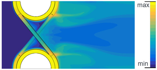
Figure 4.
Exemplary temperature field within the gas-phase of a symmetric/periodic wire mesh heat exchanger section, as obtained from CFD analysis. The inner tube surface temperature is set to . The inflow gas velocity and temperature are set to and , respectively.
For a numerical evaluation of the heat transfer, the temperatures of the gas-phase ), on the gas–solid surface (), in both solid phases, i.e., wires and tubes, (), on the coolant-side solid surface () and at the gas outlet () are calculated. The gas-side heat transfer results in
From a CFD analysis of a specific heat exchanger, heat transfer rate and temperature values appearing in Equations (29) and (21) are obtained. Accordingly, these equations can then be iteratively solved for the heat transfer coefficient and fin efficiency . In Section 3.3, correlations for and derived from the CFD results are presented.
2.4. Effective Heat Transfer Model (EM)
CFD analyses are computationally expensive and time-intensive and, therefore, not suitable for extensive parameter surveys or design optimizations. This is especially true, if successively connected layers of wired heat exchangers are to be considered, e.g., for applications where tight temperature control of chemical reactions is required. In this case, the temperature distribution along the tubes (x-direction) and of the surface temperature on the mesh surface () is of crucial importance. A CFD analysis of the prescribed case would require a very large computational domain and is impractical and depending on the gas-phase Reynolds numbers unfeasible.
For this reason, a reduced-order effective heat transfer model (EM) has been developed which is presented next.
As shown in Figure 5, the heat transfer system is separated into three phases (coolant, solid, gas) and two-phase boundary layers. The tubes and wires are considered as one phase which has one common boundary with the gas-phase . The inner surface of the tubes is represented as . Heat exchange takes only place between the individual phases described through a general approach, i.e., .
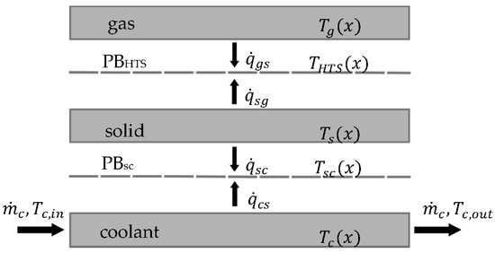
Figure 5.
Phase overview of the effective heat transfer model. All temperatures are averaged in the y- and z-directions.
Additionally, the following assumptions are made:
- Laminar flow of the gas-phase in the x-direction ;
- There are no external (thermal) sources or sinks;
- A linear driving force approach for the heat transfer is used;
- The system is in steady-state;
- In a boundary layer, energy transport takes place only by heat conduction.
By reducing the general energy Equation (25) to the flow direction (x) of the coolant, a one-dimensional equation for each phase can be derived:
With the heat transfer coefficient, the volume fraction and the mass flow rate of the corresponding phases.
All temperatures only depend on the x-coordinate and thus are comparable with the temperatures from the CFD simulations, in which the inner tube temperatures were held constant. The assumption of negligible heat losses of the heat exchanger leads to a zero gradient Neumann boundary condition for the gas-phase and the wall/solid phase in the x-direction. At the coolant entry a Dirichlet boundary condition for the inlet temperature () is used. At the outlet a zero gradient Neumann boundary condition is applied.
The boundary conditions for the system of differential equations:
The heat transfer coefficient is calculated using the correlation presented in Section 3.3 and derived from the CFD simulations.
The mean heat transfer coefficients and have also been determined from the CFD calculations and are approximated to be constant with and . Their values are significantly higher than the values of the other coefficients and thus do not limit the heat transfer. To calculate the heat transfer coefficient between coolant and tube walls a Nu-correlation given in the literature [17] is used:
Since there are six unknown temperatures and no explicit equation for , the logarithmic temperature difference in Equation (37) is used as an additional equation to solve the system of Equations (30)–(34) and (37).
After discretizing the special derivatives in the x-direction, using a central differencing scheme, and specifying the input variables , , and , the system of equations is solved using the Matlab® function fsolve [19]. All material properties are calculated as a function of temperature. This method provides heat flow for one tube. To calculate the total heat exchanger, the result must be extended by the number of tubes .
2.5. P-NTU Method
In order to quickly estimate the heat transfer over the entire heat exchanger, as well as the average outlet gas and coolant temperatures, the P-NTU [20] method is used. In addition to the EM method described in the previous section, this method provides a simple way to design heat exchangers. The overall thermal transmittance for a single tube can be calculated by using
where the thermal resistance of the solid can be approximated using Equation (39) as found in the literature [20].
For the coolant flow, we have
with given by the Nu-correlation in Equation (36). The thermal resistance of the gas flow, on the other hand, is given by
The temperature ratio
is a function of the heat capacity ratio
the number of transfer units
as well as the flow configuration, in this case a single pass counter-current flow, mixed on the coolant side.
Finally, the gas-side heat transfer and the mixed outlet temperatures and of the heat exchanger can be calculated as:
3. Results
3.1. CFD Grid Convergence Study
Following best practices, mesh independence of the CFD analysis results has to be established. Here, the Grid Convergence Index (GCI) based upon a Richardson Extrapolation as proposed in [21] or [22] has been employed in order to estimate the spatial discretization error. The first step in this approach is to calculate a representative grid length for the three-dimensional computational domain, i.e.,
where N is the overall number of grid cells and the Volume of cell . Three different computational domains with a successive grid refinement ratio are created:
This results in three different solutions and , where denotes a selected solution variable. Using the absolute errors and the pseudo-order of the computational method can be calculated iteratively, as
with
The GCI is then given by
and the estimated exact solution, as an extrapolation of the error to an infinite amount of grid cells, by
Here, the dimensionless temperature difference is used as the solution variable , with
and temperatures according to their indexed positions (see Figure 3 in this context). Figure 6 shows the results of three solutions as a function of the grid length .
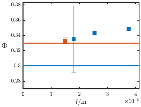
Figure 6.
Results of the grid convergence study. Nondimensional temperature versus grid length . Solutions on coarse ( ) and fine (
 ) mesh. Legend: (lines) predicted values, (squares) simulations.
) and fine () mesh. Legend: (lines) predicted values, (squares) simulations.
The result for the coarse grid with is a of 13%. This is higher than the acceptable value of 5% and therefore further grid refinement is necessary. Applying the same procedure on a refined grid with results in and thus provides sufficient accuracy of the solution with regards to the employed computational mesh.
3.2. CFD Analysis Results for Variation of Geometric Parameters
In order to determine the influences of the various geometric parameters, CFD simulations were carried out for a heat exchanger with baseline dimensions as summarized in Table 2 and by varying the inflow velocity between 0.1 and 7 m/s.
Table 2.
Geometric parameters of the heat exchanger (V1) used for parametric study together with baseline values.
The diagrams in Figure 7 show the heat transfer coefficient (a) and the pressure loss (b) as a function of inflow velocity for different values of the dimensionless diameter . As expected, heat transfer coefficients change significantly with inflow velocity, however, their variation with respect to changes in is small. The same holds true for the pressure loss across the heat exchanger. With regards to the dimensionless warp wire pitch (Figure 8), an increase in results in a lower pressure drop and a likewise decreasing heat transfer coefficient. The same behavior can also be observed for the dimensionless weft tube pitch (not illustrated).
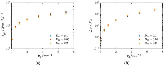
Figure 7.
Variation of heat transfer coefficient (a) and pressure loss (b) as a function of inflow velocity and dimensionless diameter ratio .
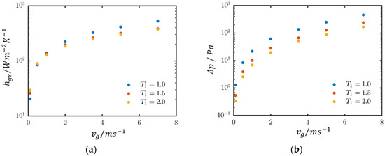
Figure 8.
Variation of heat transfer coefficient (a) and pressure loss (b) as function of inflow velocity and dimensionless warp wire pitch .
In Figure 9, the total heat flow transferred in relation to the temperature change in the gas (transmission capacity) is plotted against the pressure drop . This diagram illustrates the effect of different geometric parameter changes with respect to the baseline geometry V1 from Table 2. By increasing , a more favorable ratio of heat transfer rate to pressure drop is obtained. By increasing , the observed transmission capacity decreases more than by varying . If the dimensionless diameter is increased, the transmission capacity increases but also the pressure loss by almost the same amount. The heat transfer limitation is on the gas-side. Therefore, changes in the tube inner diameter do not have a strong influence on the heat transfer. For the sake of brevity, only a fraction of the conducted CFD analyses are discussed here. Additional details can be found in [9].
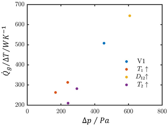
Figure 9.
Variation of heat exchanger transmission capacity and pressure drop due to changes of geometric parameters from their baseline values (V1) .
3.3. CFD-Based Eu and Nu-Correlations
Correlations for the characteristic dimensionless numbers and as defined in Equations (15) and (16) have been developed and calibrated by means of the prescribed CFD simulations. A detailed description of the procedure can be found in [9]. Table 3 shows the parameter range which was used for this purpose.
Table 3.
Parameter range considered to develop the Eu and Nu-correlations.
The predictive model for the Euler number given in Equation (55) is based on the friction factor model for straight tubes [23]:
For the Nusselt number model, a more generic approach was used. Here, is modeled as the product of power functions, each power function being represented by an influencing parameter as base and an exponent fitted by means of the CFD analyses results. This yield
Note that the Reynolds number dependency is close to that for a straight tube. The scatter plots in Figure 10 compare the fitted models with the results derived from the CFD simulations.
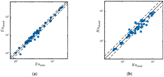
Figure 10.
Comparison between results for Euler number (a) and Nusselt number (b) obtained from CFD simulations (x-axis) and fitted models (y-axis). Legend: analysis point of parametric study, — parity, - - - - ±25% deviation.
For both Euler and Nusselt numbers good agreement between fitted models and simulation results is found. Accordingly, the correlations can be used with confidence in the technical design of heat exchanger geometries.
Figure 11 illustrates the heat exchanger transmission capacity in terms of pressure drop for the investigated geometries. These results can be fitted to a characteristic curve that can be used for the evaluation of heat exchangers of similar geometries.
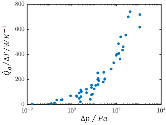
Figure 11.
Comparison of the heat exchanger transmission capacity in terms of pressure drop for a variation of heat exchanger geometric parameters.
3.4. Numerical Validation of EM and P-NTU Models
To validate the EM (effective heat transfer) model (Section 2.2) and the employed P-NTU method (Section 2.5), the performance of the heat exchanger geometry shown in Figure 4 will be calculated and compared to the results obtained from CFD analysis. The overall size of the heat exchanger is given by , , . Results are compared for the same geometric parameter variations described in Section 3.3 with a constant gas inlet temperature and variable gas inlet velocity, ranging from to . The coolant side solid surface temperature was set to for all simulations. To reach this constant temperature in the effective model, must be chosen sufficiently large.
Figure 12 shows the overall transferred heat from coolant to gas for the EM and the P-NTU method in comparison to the CFD analysis results. Differences between the effective model and the CFD simulation results are small. The relative error increases slowly with inflow gas velocity; however, it is always within the error range of the employed correlation. Deviations for the calculated temperatures are on a comparable level. For higher heat flows, the P-NTU method overestimates the results from the CFD calculations. This behavior is also found when comparing the EM model and the P-NTU method for an upscale heat exchanger, as illustrated in Figure 13. This shows a comparison of the temperatures along the pipe/tube coordinate calculated using the EM model with the mean outlet temperature determined by the P-NTU method. The overall temperature rise on the heat transfer surface is also shown. Depending on the operating point, this can lead to highly inhomogeneous temperatures in the gas-phase. This behavior can only be reproduced by the EM model. This is particularly important for the connection of several heat exchangers and thus for the overall design.
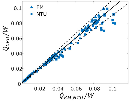
Figure 12.
Comparison of the transferred heat as predicted by CFD analysis (y-axis) and the P-NTU method or the effective heat transfer (EM) model (x-axis). Legend:  analysis point, — parity, --- ±10% deviation.
analysis point, — parity, --- ±10% deviation.
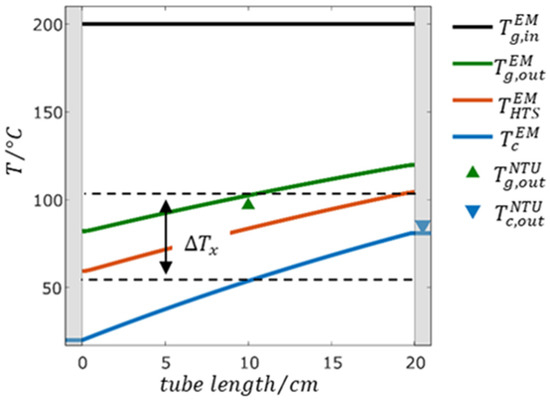
Figure 13.
Comparison of outlet temperatures calculated using the EM model and the P-NTU method. The dotted lines indicate the overall temperature increase of the heat transfer surface along the tube coordinate calculated by the EM (effective heat transfer) model.
3.5. Estimation of the Temperature Distribution on the Wire Surface
An important parameter, especially for the application of a catalytically coated heat exchanger, is the temperature distribution along the wire. Figure 14a shows this profile for a cross-section of the symmetric/periodic element used within the CFD analysis. Figure 14b illustrates the temperature variation along the wire coordinate (locally averaged over the wire cross-section) for the two simulated wires.
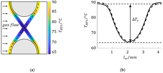
Figure 14.
Temperature distribution in (a) and along (b) the two wires calculated for geometry V1 (see Table 2) and an inflow velocity of 2.0 m/s.
Clearly, there is a significant temperature change along the wire. As a consequence, temperatures in the gas outlet are nonuniform making the design of a layered heat exchanger difficult. In addition, the prescribed temperature nonuniformities can be intensified by heat sources on the wire, for example as a result of chemical reactions. For an efficient design, the temperature difference on the wire mesh should be minimized. For this purpose, the heat conduction through the wire must be improved. The maximum temperature difference across the wire can be calculated using Equation (20) in Section 2.2. A comparison of the analytical solution (Equation (20)) with the results from CFD analysis is depicted in Figure 15, showing good agreement for different geometries. Equation (20) can therefore be used for estimating the temperature nonuniformity along the weft wire.
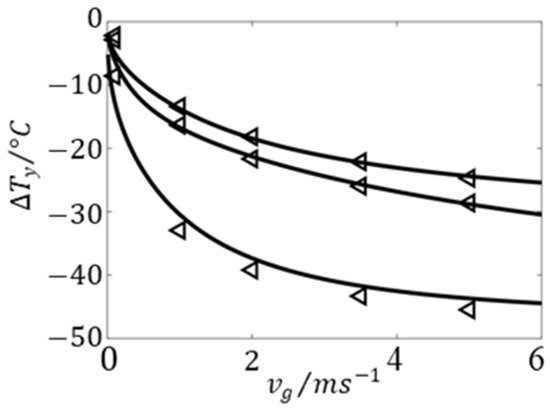
Figure 15.
Maximum temperature difference on a wire as function of inflow gas velocity and for different geometries. Comparison between analytical solutions using Equation (20) (solid lines) and values from CFD analysis (triangles).
4. Conclusions
The relevant quantities for the design of a wire cloth micro heat exchanger, consisting of a wire-screen/tubing structure, are the transmitted heat flux , the gas-phase pressure drop , the temperature rise along the tubes and the maximum temperature difference in the weft wire . Different methods were presented to calculate these quantities quickly and with high accuracy.
For the transferred heat a Nu-correlation (Equation (57) in Section 3.3) was derived based on detailed CFD analyses. The heat transfer coefficient between the outer surface and the gas, which can be calculated with this correlation, can be used to calculate the transferred heat using the P-NTU method (Equation (45) in Section 2.5). The gas-phase pressure loss is obtained from an Eu-correlation (Equation (55) in Section 3.3) which was also derived based on detailed CFD analyses. An effective 1D model (Section 2.4) was established for the temperature profiles along the tube coordinate. With this model, the nonuniformity of the temperature profiles along the heat exchanger tubes can be determined. This is relevant for the interconnection of several heat exchangers and in the presence of gas-phase or surface chemical reactions; especially in case of temperature-sensitive reactions where the use of an average temperature value may be insufficient. For the maximum temperature difference in the weft wire, an analytical estimation was found (Equation (20) in Section 2.2) which was validated by detailed CFD analyses (Section 2.3). By means of this procedure, a wire cloth heat exchanger can be designed based on the desired operating point.
Regarding the influence of geometry on pressure loss and heat transfer, an expected trend was observed. Larger distances reduce the pressure loss, but at the same time also the heat transfer. The spacing of the wires reduces the pressure loss at the transition from () to (). The increase of causes an increase in the free cross-section and thus reduces the deflection. Although the heat transfer coefficient also decreases, it does so to a much lesser extent. The diameter ratio shows a significantly lower influence compared to the tube or wire spacing. Optimization of the geometry must be carried out specifically for each design point.
The numerically determined correlations, as well as the promising application of coated heat exchangers for chemical reaction engineering, must be experimentally evaluated and validated in future work. The first experimental results for wire cloth heat exchangers were published by Fugmann et al. [3,11].
Author Contributions
Conceptualization, C.W., C.Z. and S.M.; methodology, C.W., C.Z. and S.M. software, C.W. and S.M.; validation, C.W. and S.M.; formal analysis, C.W. and S.M.; writing—original draft preparation, C.W.; writing—review and editing, U.N. and C.M.; visualization, C.W. and S.M.; supervision, U.N. and C.M.; All authors have read and agreed to the published version of the manuscript.
Funding
The authors acknowledge the financial support from the German Federal Ministry for Economic Affairs and Energy (BMWi) for the Thermogewebe Project (FKZ 03ET1281 A-D).
Acknowledgments
We acknowledge the support from Manfred Piesche from IMVT for the supervision of the numerical simulation method.
Conflicts of Interest
The authors declare no conflicts of interest.
Abbreviations
The following abbreviations are used in this manuscript:
| Greek Symbols | |
| tangential angle of contact (m) | |
| difference of a quantity | |
| logarithmic difference of a quantity | |
| volume fraction (-) | |
| numerical error | |
| fin efficiency (-) | |
| dimensionless temperature (-) | |
| dynamic viscosity (Pa s) | |
| calculation parameter for fin efficiency (-) | |
| density (kg/m3) | |
| stress tensor (kg/(ms2)) | |
| solution of numerical calculation | |
| specific surface area (m2/m3) | |
| Latin Symbols | |
| surface area (m2) | |
| heat capacity flux (W/K) | |
| heat capacity (J/(kg K)) | |
| wire diameter (m) | |
| outer tube diameter (m) | |
| inner tube diameter (m) | |
| dimensionless diameter (-) | |
| Euler number (-) | |
| Grid Convergence Index | |
| heat transfer coefficient (W/(m2 K)) | |
| interface between coolant and inner tube wall | |
| thermal conductivity (W/(m K)) | |
| interface between tube and wire | |
| distances between wires (m) | |
| distances between tubes (m) | |
| length of symmetric section (m) | |
| length of structure (m) | |
| mass flow rate (kg/s) | |
| number of grid cells (-) | |
| Nusselt number (-) | |
| number of transfer units (-) | |
| normal vector (m) | |
| number of tubes (-) | |
| number of wires (-) | |
| pressure (Pa) | |
| temperature ratio (-) | |
| phase boundary | |
| Prandtl number (-) | |
| transferred heat flux density (W/m2) | |
| transferred heat flux (W) | |
| heat capacity ratio (-) | |
| specific thermal resistance ((K m2)/(W)) | |
| Reynolds number (-) | |
| refinement ratio (-) | |
| t | time (s) |
| temperature (K) | |
| dimensionless warp wire pitch (-) | |
| dimensionless weft tube pitch (-) | |
| overall thermal transmittance (W/K) | |
| velocity (m/s) | |
| velocity vector (m/s) | |
| V | volume (m3) |
| interface between solid and gas | |
| fin coordinate (m) | |
| boundary wall in the x-direction | |
| boundary wall in the y-direction | |
| boundary wall in the z-direction | |
| Subscripts | |
| ambient condition | |
| related to the coolant phase | |
| related to the coolant-solid surface | |
| related to the curved wire | |
| related to the fin surface | |
| related to the grid | |
| related to the gas-phase | |
| related to the gas–solid surface | |
| heat exchanger | |
| related to the heat transfer surface on the air-side | |
| related to the effective heat transfer surface on the air-side | |
| inflow | |
| outflow | |
| related to the solid phase | |
| related to the solid-coolant surface | |
| related to the solid-gas surface | |
| related to the straight wire | |
| related to the tube surface | |
| related to the wire | |
| geometrical directions | |
References
- Dixit, T.; Ghosh, I. Review of micro- and mini-channel heat sinks and heat exchangers for single phase fluids. Renew. Sustain. Energy Rev. 2015, 41, 1298–1311. [Google Scholar] [CrossRef]
- Smakulski, P.; Pietrowicz, S. A review of the capabilities of high heat flux removal by porous materials, microchannels and spray cooling techniques. Appl. Therm. Eng. 2016, 104, 636–646. [Google Scholar] [CrossRef]
- Fugmann, H. Investigation of Wire Structures for Heat Transfer Enhancement in Compact Heat Exchanger. Ph.D. Thesis, Karlsruher Institut für Technologie, Karlsuhe, Germany, 2019. [Google Scholar] [CrossRef]
- Wang, Z.; Zhou, J.F.; Fan, H.L.; Shao, C.L. Experimental Study on Enhanced Heat Transfer Capability of the Array of Microtubes. Procedia Eng. 2015, 130, 250–255. [Google Scholar] [CrossRef]
- Lee, T.; Yun, J.; Lee, J.; Park, J.; Lee, K. Determination of airside heat transfer coeffcient on wire-on-tube type heat exchanger. Int. J. Heat Mass Transf. 2001, 44, 1767–1776. [Google Scholar] [CrossRef]
- Choi, S.; Cho, W.; Kim, J.; Kim, J. A study on the development of the wire woven heat exchanger using small diameter tubes. Exp. Therm. Fluid Sci. 2004, 28, 153–158. [Google Scholar] [CrossRef]
- Xu, J.; Tian, J.; Lu, T.J.; Hodson, H.P. On the thermal performance of wire-screen meshes as heat exchanger material. Int. J. Heat Mass Transf. 2007, 50, 1141–1154. [Google Scholar] [CrossRef]
- Balzer, R. Wärmetauschvorrichtung für Einen Wärmeaustausch Zwischen Medien und Webstruktur. Patent DE102006022629, 15 November 2007. [Google Scholar]
- Martens, S. Modellierung und Numerische Berechnung der Thermofluiddynamischen Eigenschaften Gewebebasierter Wärmeübertrager. Ph.D. Thesis, Universität Stuttgart, Stuttgart, Germany, 2019. [Google Scholar]
- Fugmann, H.; Laurenz, E.; Schnabel, L. Wire Structure Heat Exchangers—New Designs for Efficient Heat Transfer. Energies 2017, 10, 1341. [Google Scholar] [CrossRef]
- Fugmann, H.; Martens, S.; Balzer, R.; Brenner, M.; Schnabel, L.; Mehring, C. Performance Evaluation of Wire Cloth Micro Heat Exchangers. Energies 2020, 13, 715. [Google Scholar] [CrossRef]
- Rehman, D.; Joseph, J.; Morini, G.L.; Delanaye, M.; Brandner, J. A Hybrid numerical methodology based on CFD and porous medium for thermal performance evaluation of gas to gas micro heat exchanger. Micromachines 2020, 11, 218. [Google Scholar] [CrossRef] [PubMed]
- Kumra, A.; Rawal, N.; Samui, P. Prediction of heat transfer rate of a Wire-on-Tube type heat exchanger: An Artificial Intelligence approach. Procedia Eng. 2013, 64, 74–83. [Google Scholar] [CrossRef]
- Beshr, M.; Aute, V.; Radermacher, R. Multi-objective optimization of a residential air source heat pump with small-diameter tubes using genetic algorithms. Int. J. Refrig. 2016, 67, 134–142. [Google Scholar] [CrossRef]
- Nakaso, K.; Mitani, H.; Fukai, J. Convection heat transfer in a shell-and-tube heat exchanger using sheet fins for effective utilization of energy. Int. J. Heat Mass Transf. 2015, 82, 581–587. [Google Scholar] [CrossRef]
- Radermacher, R.; Bacellar, D.; Aute, V.; Huang, Z.; Hwang, Y.; Ling, J.; Muehlbauer, J.; Tancabel, J.; Abdelaziz, O.; Zhang, M. Miniaturized Air-to-Refrigerant Heat Exchangers; University of Maryland: College Park, MD, USA, 2017. [Google Scholar] [CrossRef]
- Shah, R.K.; London, A.L. Laminar Flow Forced Convection in Ducts: A Source Book for Compact Heat Exchanger Analytical Data; Irvine, T.F., Hartnett, J.P., Eds.; Academic Press: Cambridge, MA, USA, 2014. [Google Scholar]
- Baehr, H.D.; Stephan, K. Wärme-und Stoffübertragung; Springer: Berlin, Germany, 2016. [Google Scholar]
- MATLAB. 9.7.0.1190202 (R2019b); The MathWorks Inc.: Natick, MA, USA, 2018. [Google Scholar]
- Shah, R.K.; Sekulic, D.P. Fundamentals of Heat Exchanger Design; Wiley: Hoboken, NJ, USA, 2003. [Google Scholar]
- Roache, P.J. Perspective: A Method for Uniform Reporting of Grid Refinement Studies. J. Fluids Eng. 1994, 116, 405. [Google Scholar] [CrossRef]
- Roache, P.J. Conservatism of the Grid Convergence Index in Finite Volume Computations on Steady-State Fluid Flow and Heat Transfer. J. Fluids Eng. 2003, 125, 731. [Google Scholar] [CrossRef]
- Kopf, P.; Piesche, M.; Schütz, S. Beschreibung des Druckverlusts von Drahtgeweben mit Hilfe von Ähnlichkeitsgesetzen. Filtr. Sep. 2007, 21, 330–335. [Google Scholar]
© 2020 by the authors. Licensee MDPI, Basel, Switzerland. This article is an open access article distributed under the terms and conditions of the Creative Commons Attribution (CC BY) license (http://creativecommons.org/licenses/by/4.0/).