Abstract
To improve the trackability of in-wheel motor drive (IWMD) and wheel-individual steer electric vehicles (EVs) when steering actuators fail, the fail-operation control strategy was proposed to correct vehicles in a steering failure situation and avoid losing control of vehicle steering. A linear quadratic regulator (LQR) decides the additional yaw moment of the vehicle according to vehicle state errors. The tire force estimation module estimates the compensating resistance moment generated by the failed wheel according to the tire slip angle and the vertical tire force. By isolating the failed wheel, the optimal torque distribution (OTD) controller allocates the additional yaw moment and the compensating resistance moment to normal wheels to realize the fail-operation control of the IWMD vehicle. The control effect was verified through co-simulation of MATLAB/Simulink and Trucksim. Compared with the uncontrolled and direct torque allocation methods, the proposed OTD method reduces the lateral trajectory error of the vehicle by 86% and 60.5%, respectively, when failure occurs, and achieves better velocity maintaining ability, which proves the effectiveness of the proposed fail-operation control strategy.
1. Introduction
An in-wheel motor drive (IWMD) and wheel-individual steer vehicle removes the transmission system from traditional vehicles, and the drive torque and steering angle of each wheel can be controlled independently. Owing to the flexible layout design ability of such a vehicle, multi-axle heavy vehicles with an arbitrary number of driving and steering axles are no longer inaccessible.
Based on the characteristic of the IWMD vehicle, Jin et al. [1] proposed adaptive differential control of the IWMD vehicle to reduce the driver’s steering torque. Inspired by that, Wang et al. [2] and Wang et al. [3] presented differential drive assisted steering (DDAS), which significantly reduces a driver’s steering efforts. Giving full play to the advantages of an IWMD vehicle, Yu et al. enhanced a vehicle’s handling characteristic through joint control of DDAS and torque vectoring control [4]. Li et al. improved the stability of IWMD vehicles by distributing yaw moment error of an IWMD vehicle to four in-wheel motors [5]. For heavy trucks, Kim et al. [6,7] and Nah et al. [8] presented the drive control algorithm of a multi-axle IWMD vehicle, and computer simulations proved the feasibility of the in-wheel motor used in multi-axle vehicles.
In terms of energy efficiency and local carbon dioxide emissions of the IWMD vehicle, Sun et al. [9] proposed to reduce driving resistance by means of proper torque distribution between left and right wheels. To estimate the states of batteries and to realize the energy management of an IWMD and wheel-individual steer electric vehicle (EV), Brembeck [10] proposed a model-based state observation. Similar to [1,2,3], Jürgen et al. [11] reduced energy consumption by using the DDAS effect of the IWMD vehicle to substitute the EPS (Electric Power Steering) system.
These studies clearly show the advantages of IWMD and wheel-individual steer EVs. However, when failure occurs in a driving motor or independent steering actuation, the vehicle may deviate from the road and even cause an accident. IWMD vehicles can achieve both lateral and longitudinal dynamic vehicle control through in-wheel motor torque allocation. Therefore, it is a feasible way to improve the IWMD vehicle’s fail-operation ability by adjusting the wheel torques when a drive motor fails. In addition, when a steering actuation fails, by the isolation of failed wheel and allocating driving forces to other hub motors, we can form an additional yaw moment to steer and correct the vehicle, thus realizing the fail-operation control of the vehicle.
Nah et al. [12] used high slip ratio-based optimal control (the failed wheel rotates at a high slip rate by means of wheel torque control) to reduce lateral resistance force (the lateral force of failed wheel which would cause resistant moment when vehicle corners) of the failed wheel, which lacks the comparison of failed wheel isolation situation. On the one hand, high slip ratio causes much more energy consumption and severe tire wearout. On the other hand, high slip ratio control is heavily dependent on the precise identification of the road surface, and sudden changes of the driving force on the failed wheel will aggravate the vehicle’s instability when the road condition changes.
This contribution serves to design a new fail-operation controller when steering actuators fail and cannot steer, which isolates the failed wheel and allocates the additional yaw moment and the compensating resistance moment to normal wheels, thus reducing the lateral displacement error of the failed vehicle effectively. By evaluating the trackability of an IWMD and wheel-individual steer vehicle in the steering failure case, the proposed optimal torque distribution (OTD) control method is validated. In Section 2, the vehicle control model and the tire force estimation modular are introduced. In Section 3 and Section 4, the OTD controller is proposed to control the IWMD vehicle on the fail-operation condition, and then the results are discussed. Section 5 gives the conclusions.
2. Dynamic Models
2.1. Vehicle Control Model
Figure 1 gives the model of the IWMD and wheel-individual steer vehicle. As shown in Figure 1a, the vehicle is driven by eight in-wheel motors, and each wheel can be steered independently by the steering actuator. Figure 1b gives the parameters of the vehicle model.
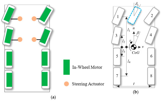
Figure 1.
Vehicle model. (a) Vehicle layout; (b) vehicle parameters.
Taking the handling characteristic of the 2-Degree-of-Freedom (2-DOF) linear vehicle model [13] as the main control target, the desired yaw rate and slip angle as the state variables, and the wheel angle of the first axle as the input, the state equation of a 2-DOF linear vehicle can be written in the form of Equation (1):
where u is the longitudinal velocity, is the moment of inertia of the vehicle about z axis, m is the vehicle mass, and is the equivalent cornering stiffness for each axle. denotes the distance between the ith axle and the vehicle’s center of gravity (CoG), which is negative for the axle behind the CoG, and H is the matrix of steering ratio from each axle to the first axle.
The steady-state gain of yaw rate and slip angle to the first axle angle is written as follows:
where
When steering failure occurs, the vehicle trajectory changes and cannot follow the driver’s steering intention. Specifically, the actual yaw rate and slip angle deviate greatly from the desired ones. In this case, the additional yaw moment can be applied to adjust the vehicle, then the state equation of the vehicle can be rewritten as follows:
where , is the additional yaw moment to correct the vehicle.
Normally, the steering angle in Equation (9) is prioritized, and the additional yaw moment acts as a backup to correct the failed vehicle.
2.2. Tire Force Estimation
The tire force estimation aims to estimate the vertical force, longitudinal force, and lateral force of tires, which will be utilized to calculate the resistance yaw moment in Section 3.2. The vertical tire force is obtained through estimation. Let us set . We can calculate the vertical tire force of the multi-axle IWMD vehicle as follows [14,15]:
where is the diagonal matrix of the equivalent tire stiffness, is the equivalent tire stiffness (the force required to raise the tire contact points with the ground by a unit travel distance when vehicle body and other wheels hold standstill), t is the track width, denotes the sprung mass, is the CoG height for sprung mass, is the roll center height, is the pitch center height, is the lateral acceleration of vehicle, is the longitudinal acceleration, and is the height of the CoG of the vehicle.
The longitudinal tire force can be obtained by Equation (15):
where the subscribe i denotes the ith wheel, is the drive torque, is the rotational inertia of the wheel, is the angular acceleration, and f is the rolling resistance coefficient of the wheel.
Considering that the failed wheel often works at a large tire slip angle, the traditional tire model formula assumption is no longer applicable, therefore, the tire model with known parameters is adopted. The tire slip angle is calculated through Equation (16). The maximum lateral tire force for a given tire slip angle when the longitudinal tire force is zero can be obtained through the lateral tire force map (see Figure 2), which is related to tire slip angle and vertical tire force.
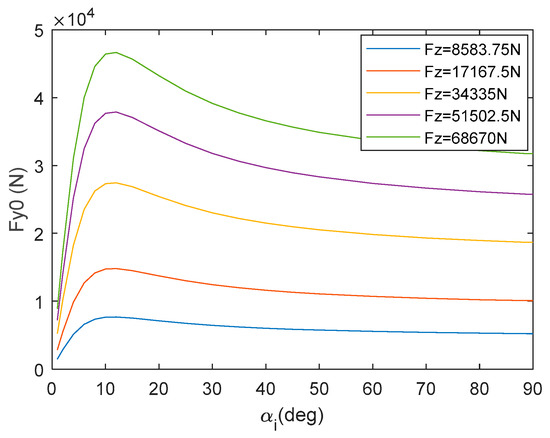
Figure 2.
Lateral tire force map in relation to the tire slip angle and vertical tire forces.
Limited by ground conditions, lateral tire force is constrained by friction ellipse expressed by Equation (17):
3. Fail-Operation Control Strategy
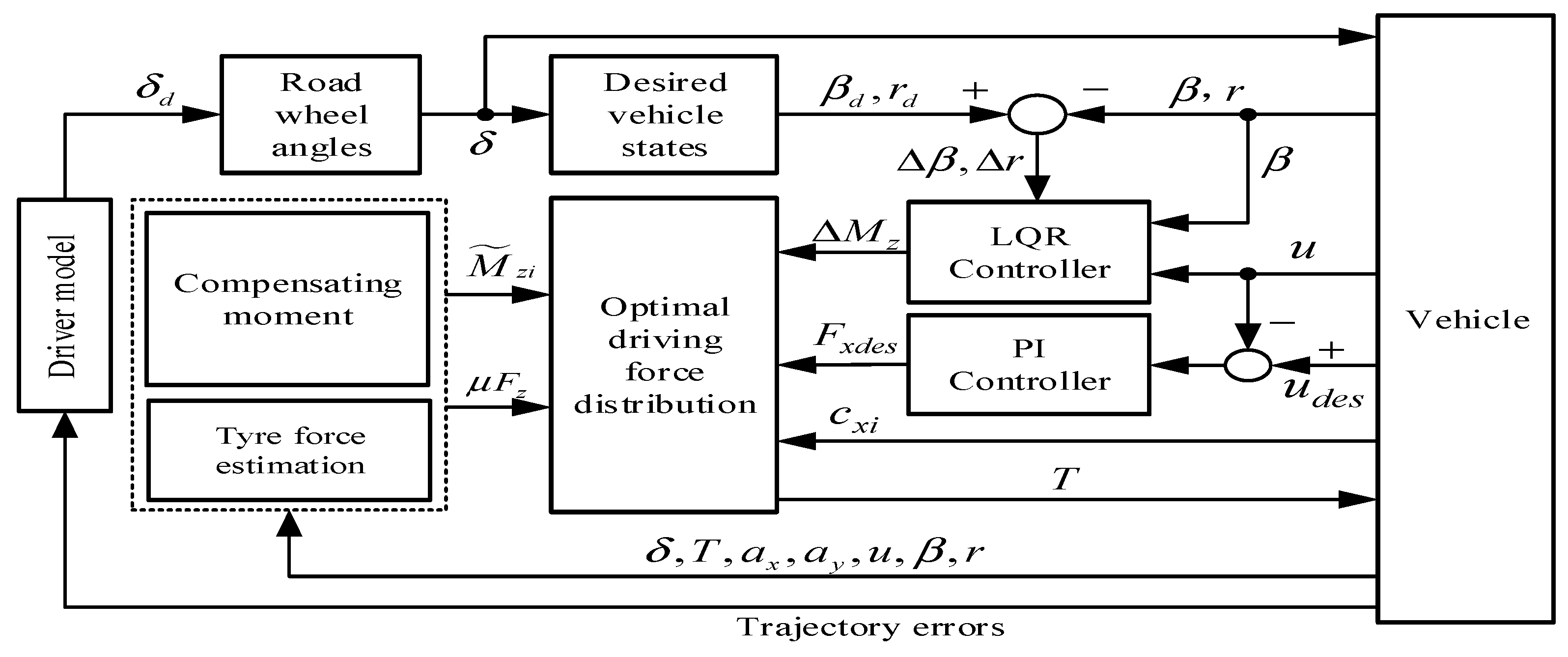
Figure 3 shows the closed-loop fail-operation control strategy for the steering failure case. The vehicle sensors are used to simulate the driver’s vision to obtain the lateral displacement error and area error of the vehicle, and the external driver model [16,17] generates the steering wheel angle accordingly. The target wheel angles can be obtained through the look-up table of the virtual gear box. The linear quadratic regulator (LQR) decides the additional yaw moment of the vehicle according to the vehicle state errors [18,19]. The PI (Proportion Integration) controller utilizes the difference between target velocity and the actual velocity to obtain the driving force. The tire force estimation module estimates the tire slip angle and vertical tire force by vehicle parameters and states, and then the lateral tire force can be obtained through the aforementioned method in Section 2.2, so as to calculate the resistance moment generated by the failed wheel. The in Figure 3 is the weight factor to isolate the failed wheel, which is set to 1 or 0 for normal and failed wheels, respectively.
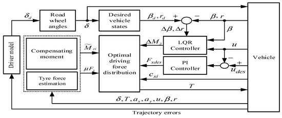
Figure 3.
Control strategy of the fail-operation steering system.
The optimal torque distribution algorithm allocates the additional yaw moment, the compensating resistance moment, and the driving force required for vehicle acceleration to the normal wheels. The adjustment of in-wheel motor torques form the vehicle yaw moment, thus finishing the closed-loop fail-operation control of the vehicle.
3.1. LQR Controller
The optimal additional yaw moment is calculated by the LQR method, and the evaluation index is established through Equation (18):
where Q and R are weight coefficient matrices.
The optimal control quantity is as follows:
The feedback coefficient K is obtained by Equation (20) and the Riccati equation (Equation (21)):
The weight coefficient matrices Q and R are given below:
where q refers to the importance attached by the evaluation index to the vehicle slip angle and the yaw rate, is the weight coefficient of the vehicle slip angle, and is the threshold value.
By solving Equation (21) offline, the table of the feedback coefficient K is obtained. Let us set , , and the optimal control yaw moment can be calculated through Equation (24) in real-time:
3.2. Optimal Tire Force Distribution
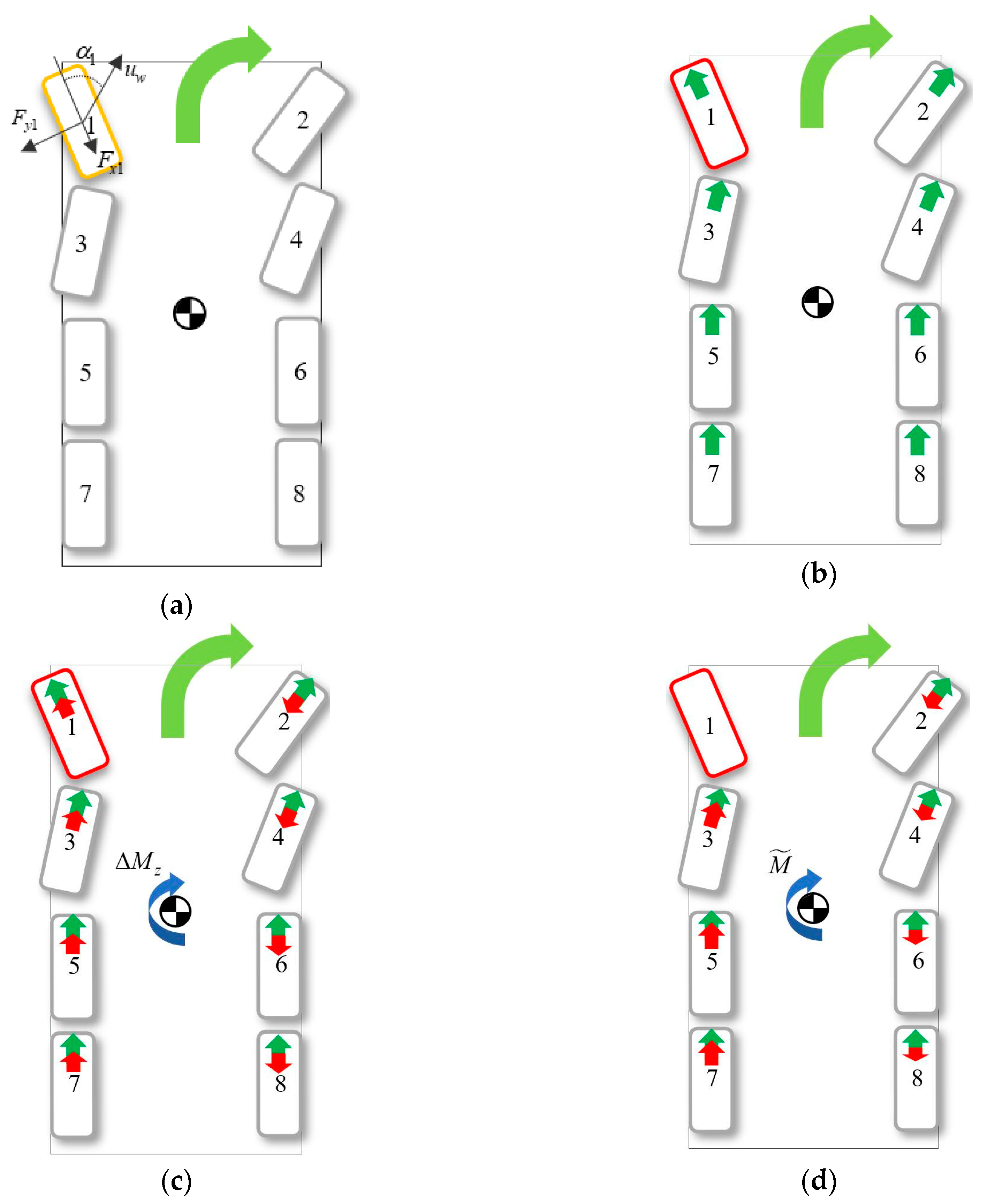
Figure 4a demonstrates the schematic diagram of an 8-wheel independent drive and a 4-wheel independent steer IWMD vehicle with the front left (No.1) wheel failed. To compare and analyze the superiority of the proposed OTD control method, four groups of vehicles are simulated here. Namely, the normal vehicle, the vehicle that operates without (w/o) any lateral control (Figure 4b), the vehicle under direct torque distribution (DTD) control (Figure 4c), and the vehicle under OTD control (Figure 4d). The green arrows in Figure 4b–d denote driving forces for accelerating, and the red arrows denote additional driving forces allocated by the corresponding controller to correct the vehicle. The DTD controller includes the additional yaw moment calculated by the LQR, and distributes the driving forces to all eight in-wheel motors numerically equal. On the basis of the DTD method, the OTD controller includes the feedforward yaw moment compensation to offset the resistance yaw moment formed by the failed wheel, but distributes the driving forces to normal wheels by isolating the failed one (No.1).
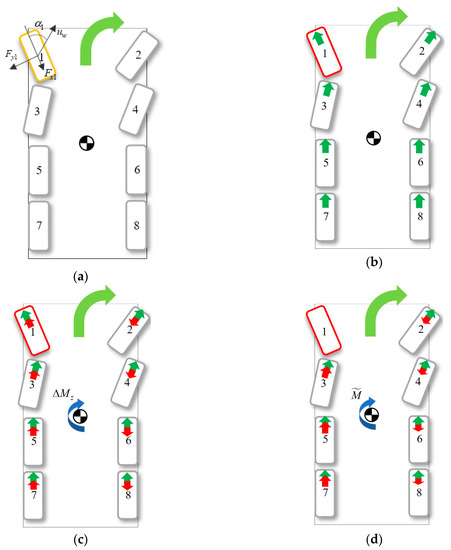
Figure 4.
Fail-operation steering of the vehicle. (a) Vehicle parameters; (b) fail-operation without lateral control; (c) fail-operation with DTD control; (d) fail-operation with OTD control.
The resistance yaw moment formed by the failed wheel is calculated by Equation (25):
The total yaw moment of the vehicle required for tracking the trajectory of the vehicle is obtained as follows:
Considering that the control object of the yaw moment is the in-wheel motor drive torque rather than the wheel angle, the weighted sum of each wheel driving force is taken as the evaluation index:
Constraints of the wheel driving forces and the additional yaw moment are as follows:
Driving forces of the rear axle wheels are expressed as a function of other wheels:
By substituting Equations (29) and (30) into Equation (27), the evaluation index function is rewritten as follows:
The necessary condition for minimizing the evaluation index is given below:
Taking wheel 1 as an example, Equation (33) can be written as follows:
For all eight wheels, we can write to state space form of Equations (34) and (35):
By solving Equation (35), state variable can be obtained, which constitutes the driving forces of the normal wheels together with the forces required to maintain the vehicle velocity:
Then, the in-wheel motor torque is obtained as follows:
4. Fail-Operation Realization
We utilized the co-simulation of MATLAB/Simulink and Trucksim software to verify the effectiveness of the controller, and the vehicle parameters are shown in Table 1. The track width of each axle is assumed to be the same. The vehicle travels at a target velocity of 30 km/h on the S road with the radius of 20 m on all curves. The left front (No.1) wheel fails when the vehicle travels 55 m in the x direction. After entering into the right turning lane, the direction of rotation for the two wheels on the first axle are opposite, so as to study the control effect for the worst failure situation.

Table 1.
Vehicle parameters.
Due to the different velocity maintaining effect of the four simulating vehicles after the steering failure, it is not intuitive to use time history to analyze the results of fail-operation, but with space history. That is, by comparing the states of vehicle under different control methods at the same trajectory point, the control effect of fail-operation is evaluated.
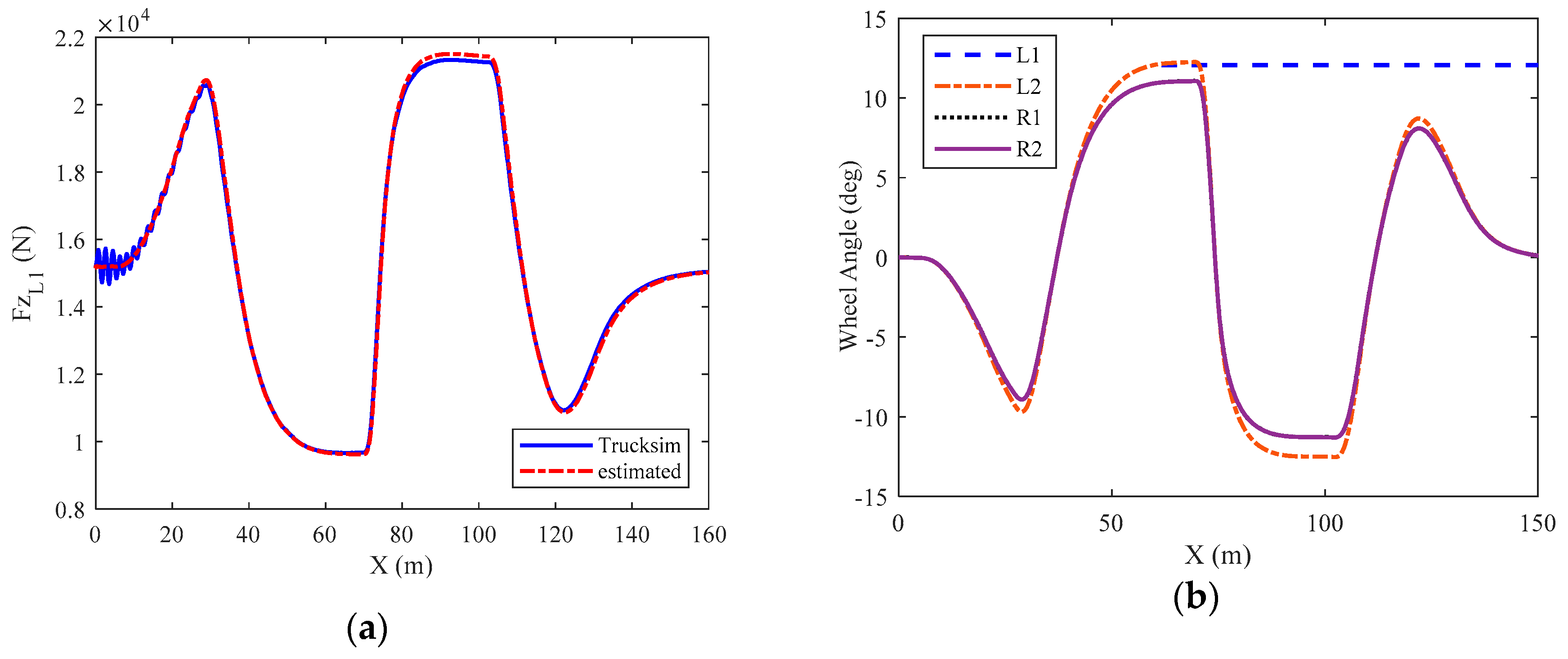
Figure 5a shows the vertical tire force of left front wheel (No.1), which demonstrates the good coincidence between the estimated vertical tire force and the Trucksim value. Figure 5b shows the wheel angle curves, which indicates that the front left wheel (L1) angle stays at an angle of 12 degrees after steering failure and other wheels operate well.
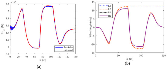
Figure 5.
Vehicle driving parameters changes. (a) Vertical tire force of the failed wheel; (b) wheel angle.
Figure 6 is the state comparation of different vehicles. According to Figure 6a,b, when the vehicle enters into the right turning lane at 75 m, the velocity of the normal vehicle maintains above 29 km/h, while that of the vehicle without control decreases to 20.5 km/h. Velocity of vehicles under DTD control and OTD control are 24 km/h and 25.5 km/h, respectively, and the results illustrate the good velocity control effect of the OTD control method.
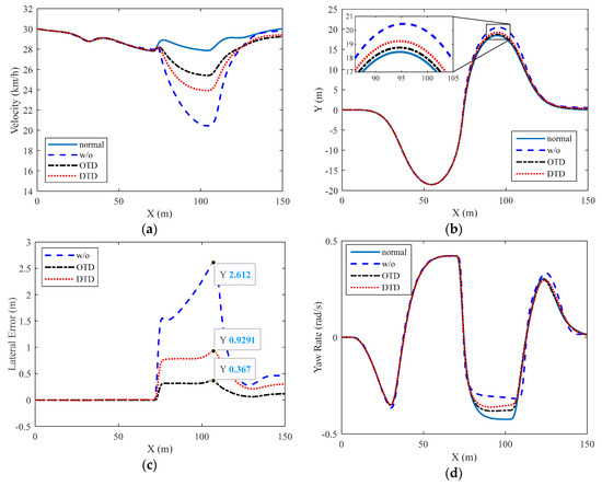
Figure 6.
State comparation of different vehicles. (a) Vehicle velocity; (b) vehicle trajectory; (c) lateral displacement error relative to normal vehicle; (d) vehicle yaw rate.
To furtherly investigate the effectiveness of the proposed OTD control method, the lateral displacement enhance rate (LDER, the reduction rate of maximum lateral displacement error of vehicle under different control methods compared with vehicle without control) is defined and calculated in terms of the peak value of the lateral displacement error as follows:
where denotes the lateral displacement error of either DTD controlled vehicle or vehicle without control.
As shown in Figure 6c,d, comparing with the normal vehicle, the peak value of the lateral displacement error reaches 2.612 m, 0.929 m, and 0.367 m for vehicle without control (w/o), under DTD control, and under OTD control, respectively. In other words, the LDER of the OTD controlled vehicle is 86% and 60.5% compared with the vehicle without control (w/o) and under DTD control, respectively. The yaw rate curves in Figure 6d demonstrate that the vehicle under OTD control follows the normal vehicle best before and after corning.
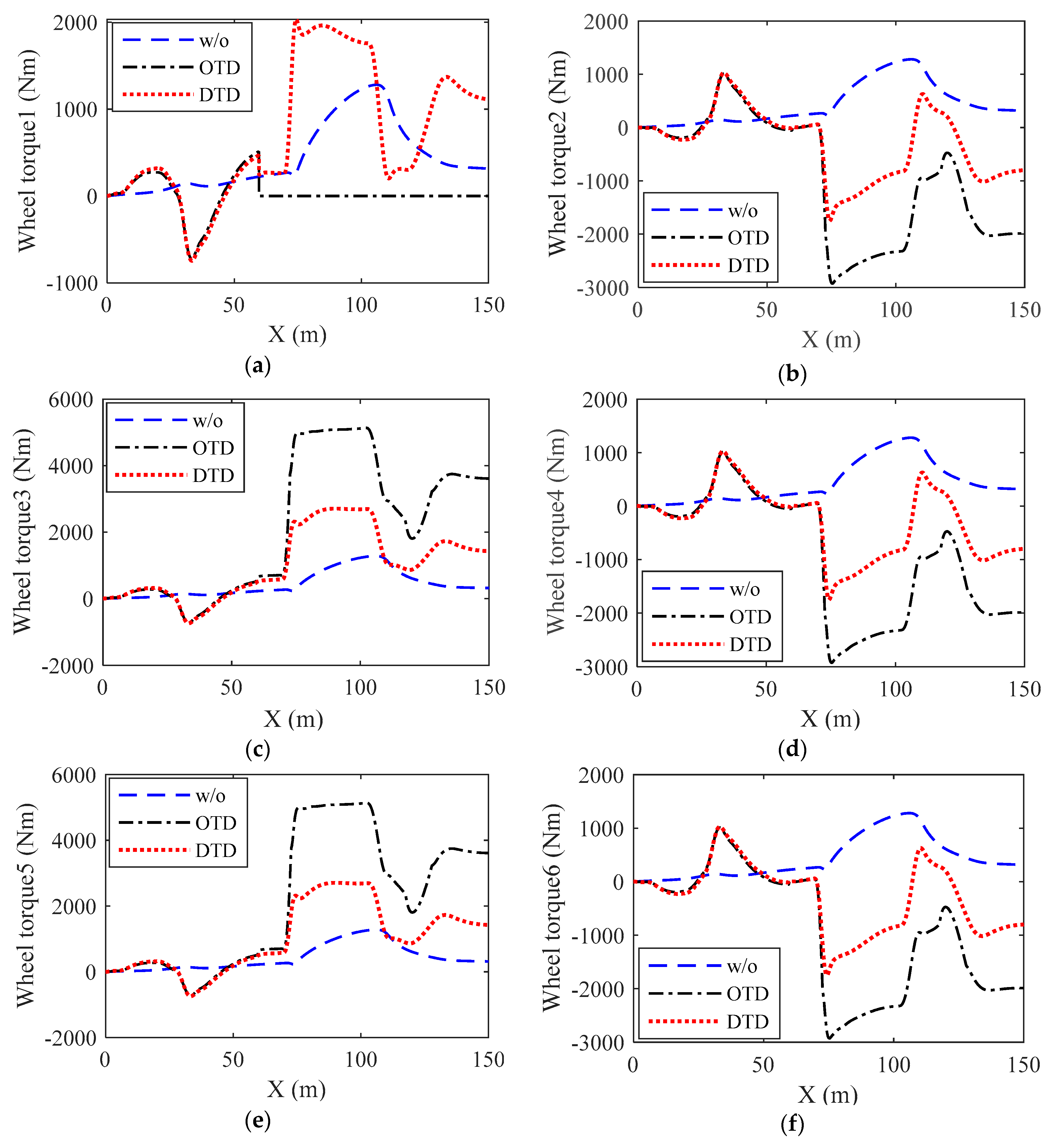
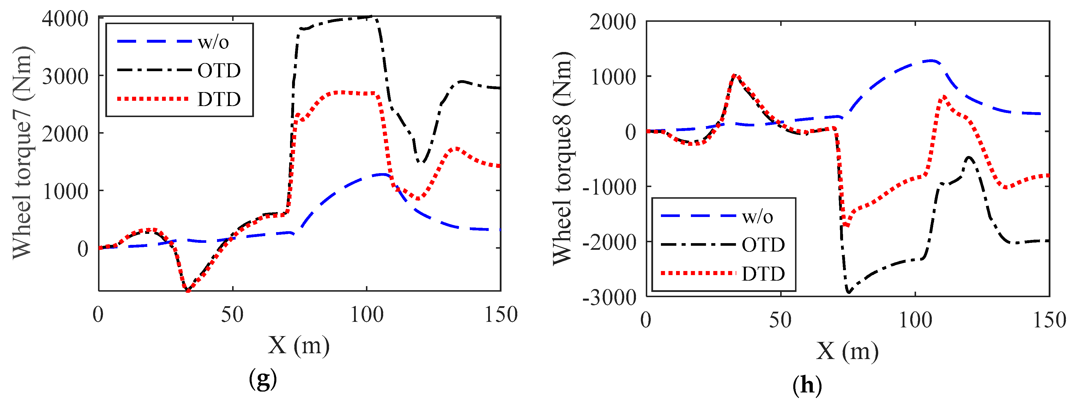
Figure 7 shows the wheel torque for different control methods. The wheels numbered 1, 3, 5, and 7 are on the left side (see Figure 4) of the vehicle, and the wheels numbered 2, 4, 6, and 8 are on the right side. It can be observed that the eight in-wheel motor torques are equal for EVs without fail-operation control. As for the vehicle under DTD control, the eight in-wheel motor torques on both sides are different because of the requirement to form the additional yaw moment to correct the vehicle.
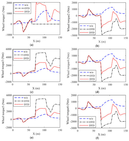
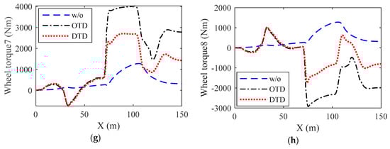
Figure 7.
Wheel torque for different control methods. (a) Torque of wheel No.1; (b) torque of wheel No.2; (c) torque of wheel No.3; (d) torque of wheel No.4; (e) torque of wheel No.5; (f) torque of wheel No.6; (g) torque of wheel No.7; (h) torque of wheel No.8.
Different from the vehicle under DTD control, the torque on the failed wheel 1 is zero for OTD controlled vehicle when failure occurs, and thus avoids energy consumption and reduces the disturbance of the driving force on this wheel. Due to the absence of the driving force on the failed wheel and to form the required yaw moment for trajectory correction, drive torques of the normal wheels on the failure side (left side) are significantly larger than that of the normal side (right side).
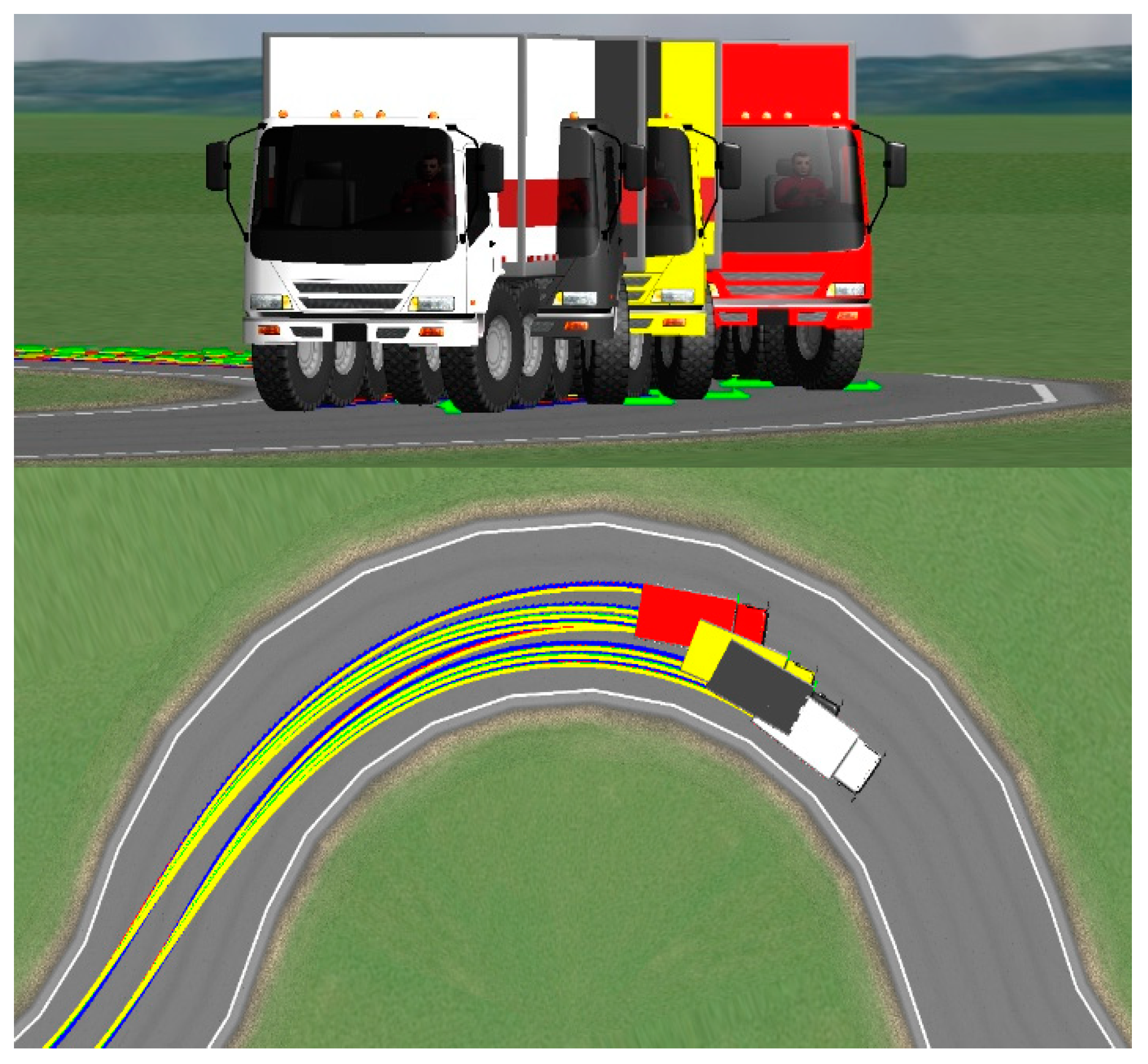
It can be seen more intuitively from the trajectory animation in Figure 8 that vehicles under different control methods separate after entering the right turning lane. The innermost white vehicle is the normal vehicle. The outermost red vehicle is the fail-operation vehicle without control. The second outermost vehicle in yellow is the vehicle under DTD control, and the black vehicle next to the normal one is the vehicle under OTD control. It shows that the direction of the left front and right front wheels are opposite for all failed vehicles, and the vehicle without control travels with the largest trajectory deviation and the slowest velocity.

Figure 8.
Animation of the trajectories of different vehicles.
Compared with the vehicles without control and under DTD control, the OTD controlled vehicle can significantly reduce the tracking error along with the best velocity maintaining ability, which verifies the effectiveness of the proposed fail-operation control strategy.
5. Conclusions
- (1)
- To improve the fail-operation ability of IWMD and wheel independent steering vehicles, a fail-operation control strategy through failed wheel isolation and yaw moment compensation is proposed based on the optimal driving force distribution. When steering failure occurs, the LQR utilizes the vehicle side-slip angle deviations and yaw rate to decide the additional yaw moment of the vehicle. The tire force estimation modular estimates the lateral tire force of the failed wheel to calculate the resisting yaw moment. The optimal driving force distribution controller isolates the failed wheel and allocates the additional vehicle yaw moment and the estimated wheel resisting yaw moment to normal driving wheels to correct the vehicle.
- (2)
- By means of joint simulation of Trucksim and MATLAB/Simulink, the effectiveness of the proposed control strategy was verified. Results showed that the optimal distribution of the driving force reduced the lateral trajectory deviation of the fail-operation vehicle by 86% and 60.5%, respectively, compared with the vehicles without control and under DTD control, which enhanced the road tracing ability of the fault vehicle. Meanwhile, the proposed OTD controlled vehicle showed great superiority in terms of velocity maintaining.
- (3)
- Fault diagnosis and identification will be studied in the future to pave way for the experimental test, and furtherly validate the proposed fail-operation control strategies.
Author Contributions
Conceptualization, Z.Z. and J.L.; methodology, Z.Z.; software, Z.Z. and J.W.; validation, Z.Z. and L.J.; data curation, Z.Z.; writing, Z.Z., J.L. and J.W.; supervision, L.J.; project administration, L.J. All authors have read and agreed to the published version of the manuscript.
Funding
This research was funded by the National Natural Science Foundation of China (Grant No. 51875235) and the Natural Science Foundation of Jilin Province (Grant No.: 20170101208JC), and in part by the Jilin Province Science and Technology Development Project under Grant 20180414011GH.
Conflicts of Interest
The authors declare no conflicts of interest.
References
- Jin, L.Q.; Wang, Q.N.; Zhang, H.H.; Wang, J.N. A study on differential technology of in-wheel motor drive EV. Automot. Eng. 2007, 29, 700–704. [Google Scholar]
- Wang, Q.N.; Wang, J.N.; Jin, L.Q. Differential assisted steering applied on electric vehicle with electric motorized wheels. J. Jilin Univ. (Eng. Technol. Ed.) 2010, 39, 1–6. [Google Scholar]
- Wang, J.; Wang, Q.; Jin, L.; Song, C. Independent wheel torque control of 4WD electric vehicle for differential drive assisted steering. Mechatronics 2011, 21, 63–76. [Google Scholar] [CrossRef]
- Yu, Z.P.; Liu, J.; Xiong, L.; Feng, Y. Control strategies of handling improvement of distributed drive electric vehicle. J. Tongji Univ. (Nat. Sci.) 2014, 42, 1088–1095. [Google Scholar]
- Li, B.; Goodarzi, A.; Khajepour, A. An optimal torque distribution control strategy for four-independent wheel drive electric vehicles. Veh. Syst. Dyn. 2015, 53, 1172–1189. [Google Scholar] [CrossRef]
- Kim, W.G.; Yi, K.; Lee, J. Drive control algorithm for an independent 8 in-wheel motor drive vehicle. J. Mech. Sci. Technol. 2011, 25, 1573–1581. [Google Scholar] [CrossRef]
- Kim, W.G.; Kang, J.Y.; Yi, K. Drive control system design for stability and maneuverability of a 6WD/6WS vehicle. Int. J. Automot. Technol. 2011, 12, 67–74. [Google Scholar] [CrossRef]
- Nah, J.; Seo, J.; Yi, K.; Kim, W.G.; Lee, J. Friction circle estimation-based torque distribution control of six-wheeled independent driving vehicles for terrain-driving performance. Proc. Inst. Mech. Eng. Part D J. Automob. Eng. 2015, 229, 1469–1482. [Google Scholar] [CrossRef]
- Sun, W.; Wang, Q.N.; Wang, J.N. Yaw-moment control of motorized vehicle for energy conservation during cornering. J. Jilin Univ. (Eng. Technol. Ed.) 2018, 48, 11–19. [Google Scholar]
- Brembeck, J. Model Based Energy Management and State Estimation for the Robotic Electric Vehicle ROboMObil. Ph.D. Thesis, Electrical Engineering and Information Technology College of Technical University of Munich, Munich, Germany, 2018. [Google Scholar]
- Jürgen, R.; Philipp, K.; Michael, F.; Frank, G. Reducing energy demand using wheel-individual electric drives to substitute EPS-systems. Energies 2018, 11, 247. [Google Scholar]
- Nah, J.; Kim, W.; Yi, K.; Lee, D.; Lee, J. Fault-tolerant driving control of a steer-by-wire system for six-wheel-driving-six-wheel-steering vehicle. Proc. Inst. Mech. Eng. Part D J. Automob. Eng. 2013, 227, 506–520. [Google Scholar] [CrossRef]
- Daniel, W. Generalized multi-axle vehicle handling. Veh. Syst. Dyn. 2012, 50, 149–166. [Google Scholar]
- Liu, W.; He, H.W.; Sun, F.C.; Lv, J.Y. Integrated chassis control for a three-axle electric bus with distributed driving motors and active rear steering system. Veh. Syst. Dyn. 2017, 55, 601–625. [Google Scholar] [CrossRef]
- Zhang, Y.B.; Khajepour, A.; Huang, Y.J. Multi-axle/articulated bus dynamics modeling: A reconfigurable approach. Veh. Syst. Dyn. 2018, 56, 1315–1343. [Google Scholar] [CrossRef]
- Plöchl, M.; Edelmann, J. Driver models in automobile dynamics application. Veh. Syst. Dyn. 2007, 45, 699–741. [Google Scholar] [CrossRef]
- Ungoren, A.Y.; Peng, H. An adaptive lateral preview driver model. Veh. Syst. Dyn. 2005, 43, 245–259. [Google Scholar] [CrossRef]
- Kırlı, A.; Chen, Y.S.; Okwudire, C.E.; Ulsoy, A.G. Torque-vectoring-based backup steering strategy for steer-by-wire autonomous vehicles with vehicle stability control. IEEE Trans. Veh. Technol. 2019, 68, 7319–7328. [Google Scholar] [CrossRef]
- Ding, H.T.; Guo, K.H.; Chen, H. LQR method for vehicle yaw moment decision in vehicle stability control. J. Jilin Univ. (Eng. Technol. Ed.) 2010, 40, 597–601. [Google Scholar]


© 2020 by the authors. Licensee MDPI, Basel, Switzerland. This article is an open access article distributed under the terms and conditions of the Creative Commons Attribution (CC BY) license (http://creativecommons.org/licenses/by/4.0/).