Power Optimization of a Modified Closed Binary Brayton Cycle with Two Isothermal Heating Processes and Coupled to Variable-Temperature Reservoirs


Abstract
1. Introduction
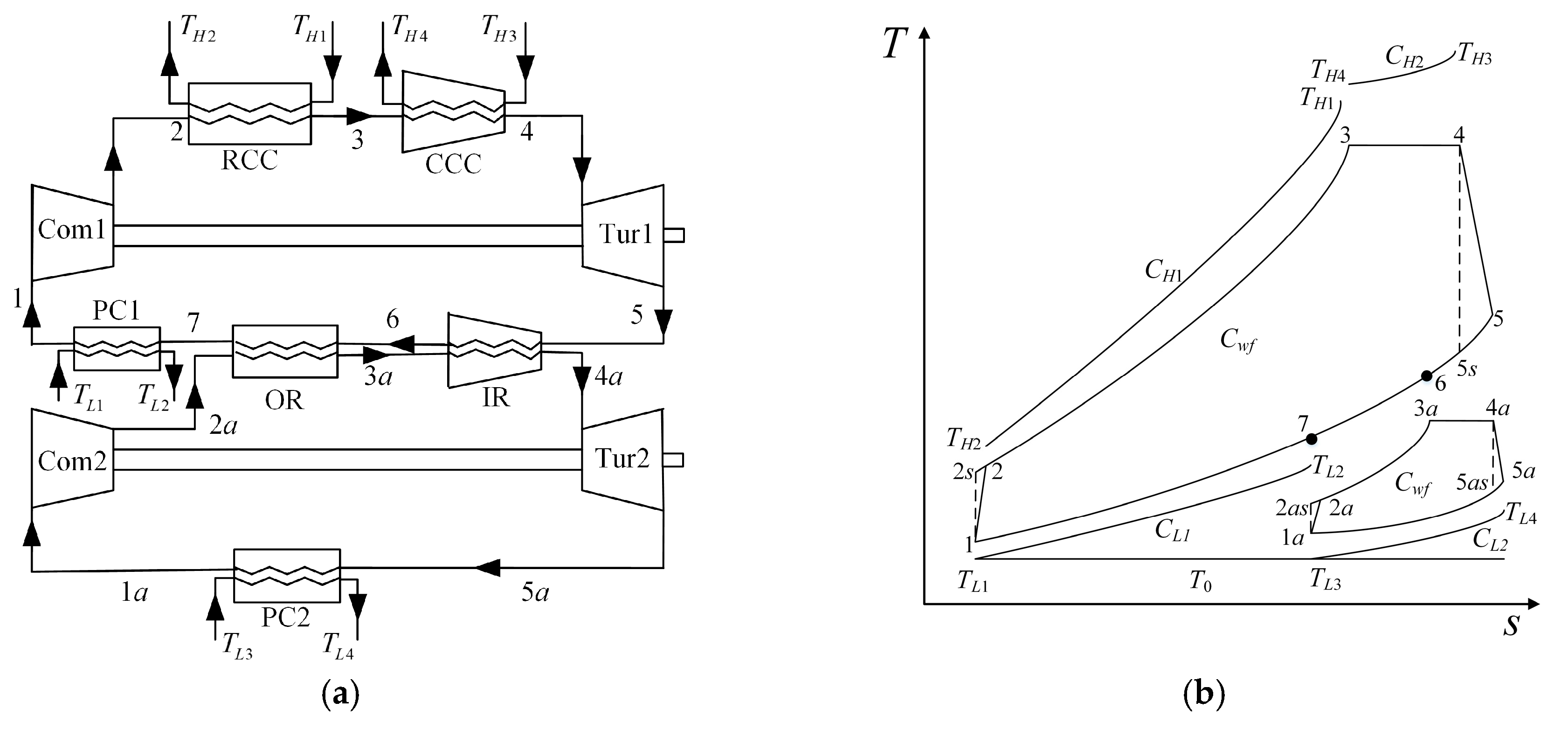
2. Cycle Model
3. Optimal Heat Conductance Distributions
4. Optimal Thermal Capacitance Rate Matchings
5. Conclusions
Author Contributions
Funding
Acknowledgments
Conflicts of Interest
Nomenclature
| a, b, c, d, e, m, x, y | Intermediate variables |
| C | Thermal capacity rate (kW/K) |
| Cp | Specific heat at constant pressure (kJ/(kg·K)) |
| E | Effectiveness of heat exchanger |
| k | Specific heat ratio |
| M | Mach number |
| N | Number of heat transfer units |
| Heat absorbing rate or heat releasing rate | |
| Rg | Gas constant (kJ/(kg·K)) |
| T | Temperature (K) |
| U | Heat conductance (kW/K) |
| u | Heat conductance distribution |
| W | Power output(kW) |
| Dimensionless power output | |
| Greek symbol | |
| Efficiency | |
| π | Pressure ratio |
| Temperature ratio | |
| Subscripts | |
| bot | Bottoming cycle |
| com | Compressor |
| H | Hot-side heat exchanger |
| L | Cold-side heat exchanger |
| R | Regenerator |
| s | Isentropic |
| t/ta | Converging combustion chamber/isothermal regenerator |
| tot | Total |
| tur | Turbine |
| top | Topping cycle |
| wf | Working fluid |
| 1,2,3,4,5,6,7,1a,2a,3a,4a,5a,2s,5s,2as,5as | State points |
Abbreviations
| CCC | Converging combustion chamber |
| CTR | Constant-temperature reservoir |
| FTT | Finite-time thermodynamics |
| HCD | Heat conductance distribution |
| IR | Isothermal regenerator |
| MCBBC | Modified closed binary Brayton cycle |
| PO | Power output |
| PD | Power density |
| OR | Ordinary regenerator |
| RCC | Regular combustion chamber |
| TCRM | Thermal capacitance rate matching |
| TEF | Thermal efficiency |
| THC | Total heat conductance |
| Tur | Turbine |
| VTHR | Variable-temperature heat reservoir |
| WF | Working fluid |
Appendix A
References
- Invernizzi, C.M. Prospects of mixtures as working fluids in real-gas Brayton cycles. Energies 2017, 10, 1649. [Google Scholar] [CrossRef]
- Wang, J.P.; Wang, J.; Lund, P.D.; Zhu, H.X. Thermal performance analysis of a direct-heated recompression supercritical carbon dioxide Brayton cycle using solar concentrators. Energies 2019, 12, 4358. [Google Scholar] [CrossRef]
- Jaszczur, M.; Dudek, M.; Kolenda, Z. Thermodynamic analysis of advanced gas turbine combined cycle integration with a high-temperature nuclear reactor and cogeneration unit. Energies 2020, 13, 400. [Google Scholar] [CrossRef]
- Vecchiarelli, J.; Kawall, J.G.; Wallace, J.S. Analysis of a concept for increasing the efficiency of a Brayton cycle via isothermal heat addition. Int. J. Energy Res. 1997, 21, 113–127. [Google Scholar] [CrossRef]
- Göktun, S.; Yavuz, H. Thermal efficiency of a regenerative Brayton cycle with isothermal heat addition. Energy Convers. Manag. 1999, 40, 1259–1266. [Google Scholar] [CrossRef]
- Erbay, L.B.; Göktun, S.; Yavuz, H. Optimal design of the regenerative gas turbine engine with isothermal heat addition. Appl. Energy 2001, 68, 249–264. [Google Scholar] [CrossRef]
- Jubeh, N.M. Exergy analysis and second law efficiency of a regenerative Brayton cycle with isothermal heat addition. Entropy 2005, 7, 172–187. [Google Scholar] [CrossRef]
- El-Maksound, R.M.A. Binary Brayton cycle with two isothermal processes. Energy Convers. Manag. 2013, 73, 303–308. [Google Scholar] [CrossRef]
- Qi, W.; Wang, W.H.; Chen, L.G. Exergy analysis and optimization for binary Brayton cycle with two isothermal heat additions. Therm. Turbine 2017, 46, 76–81. (In Chinese) [Google Scholar]
- Andresen, B.; Salamon, P.; Barry, R.S. Thermodynamics in finite time. Phys. Today 1987, 37, 62–70. [Google Scholar] [CrossRef]
- Chen, L.G.; Li, J. Thermodynamic optimization theory for Two-Heat-Reservoir cycles; Science Press: Beijing, China, 2020. [Google Scholar]
- Barranco-Jimenez, M.A.; Ramos-Gayosso, I.; Rosales, M.A.; Angulo-Brown, F. A proposal of ecologic taxes based on thermoeconomic performance of heat engine models. Energies 2009, 2, 1042–1056. [Google Scholar] [CrossRef]
- Chen, C.L.; Ho, C.E.; Yau, H.T. Performance analysis and optimization of a solar powered Stirling engine with heat transfer considerations. Energies 2012, 5, 3573–3585. [Google Scholar] [CrossRef]
- Gonca, G. Energy and exergy analyses of single and double reheat irreversible Rankine cycle. Int. J. Exergy 2015, 18, 402–422. [Google Scholar] [CrossRef]
- Han, Z.H.; Li, P.; Han, X.; Mei, Z.K.; Wang, Z. Thermo-economic performance analysis of a regenerative superheating organic Rankine cycle for waste heat recovery. Energies 2017, 10, 1593. [Google Scholar] [CrossRef]
- White, M.T.; Sayma, A.I. A generalised assessment of working fluids and radial turbines for non-recuperated subcritical organic Rankine cycles. Energies 2018, 11, 800. [Google Scholar] [CrossRef]
- Chen, W.J.; Feng, H.J.; Chen, L.G.; Xia, S.J. Optimal performance characteristics of subcritical simple irreversible organic Rankine cycle. J. Therm. Sci. 2018, 27, 555–562. [Google Scholar] [CrossRef]
- Vittorini, D.; Cipollone, R.; Carapellucci, R. Enhanced performances of ORC-based units for low grade waste heat recovery via evaporator layout optimization. Energy Convers. Manag. 2019, 197, 111874. [Google Scholar] [CrossRef]
- Koo, J.; Oh, S.R.; Choi, Y.U.; Jung, J.H.; Park, K. Optimization of an organic Rankine cycle system for an LNG-powered ship. Energies 2019, 12, 1933. [Google Scholar] [CrossRef]
- Wang, S.; Zhang, W.; Feng, Y.Q.; Wang, X.; Wang, Q.; Liu, Y.Z.; Wang, Y.; Yao, L. Entropy, entransy and exergy analysis of a dual-loop organic Rankine cycle (DORC) using mixture working fluids for engine waste heat recovery. Energies 2020, 13, 1301. [Google Scholar] [CrossRef]
- Feng, H.J.; Chen, W.J.; Chen, L.G.; Tang, W. Power and efficiency optimizations of an irreversible regenerative organic Rankine cycle. Energy Convers. Manag. 2020, 220, 113079. [Google Scholar] [CrossRef]
- Chen, L.G.; Ma, K.; Feng, H.J.; Ge, Y.L. Optimal configuration of a gas expansion process in a piston-type cylinder with generalized convective heat transfer law. Energies 2020, 13, in press. [Google Scholar]
- Chen, L.G.; Meng, F.K.; Sun, F.R. Thermodynamic analyses and optimizations for thermoelectric devices: the state of the arts. Sci. China Technol. Sci. 2016, 59, 442–455. [Google Scholar] [CrossRef]
- Chen, J.L.; Li, K.W.; Liu, C.W.; Li, M.; Lv, Y.C.; Jia, L.; Jiang, S.S. Enhanced efficiency of thermoelectric generator by optimizing mechanical and electrical structures. Energies 2017, 10, 1329. [Google Scholar] [CrossRef]
- Feng, Y.L.; Chen, L.G.; Meng, F.K.; Sun, F.R. Influences of external heat transfer and Thomson effect on performance of TEG-TEC combined thermoelectric device. Sci. China Technol. Sci. 2018, 61, 1600–1610. [Google Scholar] [CrossRef]
- Li, G.; Wang, Z.C.; Wang, F.; Wang, X.Z.; Li, S.B.; Xue, M.S. Experimental and numerical study on the effect of interfacial heat transfer on performance of thermoelectric generators. Energies 2019, 12, 3797. [Google Scholar] [CrossRef]
- Açıkkalp, E.; Chen, L.G.; Ahmadi, M.H. Comparative performance analyses of molten carbonate fuel cell-alkali metal thermal to electric converter and molten carbonate fuel cell –thermoelectric generator hybrid systems. Energy Rep. 2020, 6, 10–16. [Google Scholar] [CrossRef]
- Gonca, G. Exergetic and thermo-ecological performance analysis of a Gas-Mercury combined turbine system (GMCTS). Energy Convers. Manag. 2017, 151, 32–42. [Google Scholar] [CrossRef]
- Lin, J.; Zhang, Z.H.; Zhu, X.Y.; Meng, C.; Li, N.; Chen, J.C.; Zhao, Y.R. Performance evaluation and parametric optimization strategy of a thermocapacitive heat engine to harvest low-grade heat. Energy Convers. Manag. 2019, 184, 40–47. [Google Scholar] [CrossRef]
- Zhu, F.L.; Chen, L.G.; Wang, W.H. Thermodynamic analysis and optimization of irreversible Maisotsenko-Diesel cycle. J. Therm. Sci. 2019, 28, 659–668. [Google Scholar] [CrossRef]
- Dumitrascu, G.; Feidt, M.; Popescu, A.; Grigorean, S. Endoreversible trigeneration cycle design based on finite physical dimensions thermodynamics. Energies 2019, 12, 3165. [Google Scholar]
- Wu, Z.X.; Chen, L.G.; Feng, H.J. Thermodynamic optimization for an endoreversible Dual-Miller cycle (DMC) with finite speed of piston. Entropy 2018, 20, 165. [Google Scholar] [CrossRef]
- You, J.; Chen, L.G.; Wu, Z.X.; Sun, F.R. Thermodynamic performance of Dual-Miller cycle (DMC) with polytropic processes based on power output, thermal efficiency and ecological function. Sci. China Technol. Sci. 2018, 61, 453–463. [Google Scholar] [CrossRef]
- Abedinnezhad, S.; Ahmadi, M.H.; Pourkiaei, S.M.; Pourfayaz, F.; Mosavi, A.; Feidt, M.; Shamshirband, S. Thermodynamic assessment and multi-objective optimization of performance of irreversible Dual-Miller cycle. Energies 2019, 12, 4000. [Google Scholar] [CrossRef]
- Ding, Z.M.; Ge, Y.L.; Chen, L.G.; Feng, H.J.; Xia, S.J. Optimal performance regions of Feynman’s ratchet engine with different optimization criteria. J. Non-Equilib. Thermodyn. 2020, 45, 191–207. [Google Scholar] [CrossRef]
- Feng, H.J.; Qin, W.X.; Chen, L.G.; Cai, C.G.; Ge, Y.L.; Xia, S.J. Power output, thermal efficiency and exergy-based ecological performance optimizations of an irreversible KCS-34 coupled to variable temperature heat reservoirs. Energy Convers. Manag. 2020, 205, 112424. [Google Scholar] [CrossRef]
- Chen, L.G.; Sun, F.R.; Wu, C. Performance analysis of an irreversible Brayton heat engine. J. Inst. Energy 1997, 70, 2–8. [Google Scholar]
- Sadatsakkak, S.A.; Ahmadi, M.H.; Ahmadi, M.A. Thermodynamic and thermo-economic analysis and optimization of an irreversible regenerative closed Brayton cycle. Energy Convers. Manag. 2015, 94, 124–129. [Google Scholar] [CrossRef]
- Naserian, M.M.; Farahat, S.; Sarhaddi, F. Finite time exergy analysis and multi-objective ecological optimization of a regenerative Brayton cycle considering the impact of flow rate variations. Energy Convers. Manag. 2015, 103, 790–800. [Google Scholar] [CrossRef]
- Jansen, E.; Bello-Ochende, T.; Meyer, J.P. Integrated solar thermal Brayton cycles with either one or two regenerative heat exchangers for maximum power output. Energy 2015, 86, 737–748. [Google Scholar] [CrossRef]
- Sánchez-Orgaz, S.; Medina, A.; Calvo Hernández, A. Thermodynamic model and optimization of a multi-step irreversible Brayton cycle. Energy Convers. Manag. 2010, 51, 2134–2143. [Google Scholar] [CrossRef]
- Sanchez-Orgaz, S.; Pedemonte, M.; Ezzatti, P.; Curto-Risso, P.L.; Medina, A.; Calvo Hernández, A. Multi-objective optimization of a multi-step solar-driven Brayton plant. Energy Convers. Manag. 2015, 99, 346–358. [Google Scholar] [CrossRef]
- Chen, L.G.; Feng, H.J.; Ge, Y.L. Power and efficiency optimization for open combined regenerative Brayton and inverse Brayton cycles with regeneration before the inverse cycle. Entropy 2020, 22, 677. [Google Scholar] [CrossRef]
- Açıkkalp, E. Performance analysis of irreversible solid oxide fuel cell–Brayton heat engine with ecological based thermo-environmental criterion. Energy Convers. Manag. 2017, 148, 279–286. [Google Scholar] [CrossRef]
- Zhu, F.L.; Chen, L.G.; Wang, W.H. Thermodynamic analysis of an irreversible Maisotsenko reciprocating Brayton cycle. Entropy 2018, 20, 167. [Google Scholar] [CrossRef]
- Chen, L.G.; Shen, J.F.; Ge, Y.L.; Wu, Z.X.; Wang, W.H.; Zhu, F.L.; Feng, H.J. Power and efficiency optimization of open Maisotsenko-Brayton cycle and performance comparison with traditional open regenerated Brayton cycle. Energy Convers. Manag. 2020, 217, 113001. [Google Scholar] [CrossRef]
- Feng, H.J.; Tao, G.S.; Tang, C.Q.; Ge, Y.L.; Chen, L.G.; Xia, S.J. Exergoeconomic performance optimization for a regenerative gas turbine closed-cycle heat and power cogeneration plant. Energy Rep. 2019, 5, 1525–1531. [Google Scholar] [CrossRef]
- Chen, L.G.; Yang, B.; Feng, H.J.; Ge, Y.L.; Xia, S.J. Performance optimization of an open simple-cycle gas turbine combined cooling, heating and power plant driven by basic oxygen furnace gas in China’s steelmaking plants. Energy 2020, 203, 117791. [Google Scholar] [CrossRef]
- Kaushik, S.C.; Tyagi, S.K.; Singhal, M.K. Parametric study of an irreversible regenerative Brayton cycle with isothermal heat addition. Energy Convers. Manag. 2003, 44, 2013–2025. [Google Scholar] [CrossRef]
- Tyagi, S.K.; Kaushik, S.C.; Tiwari, V. Ecological optimization and parametric study of an irreversible regenerative modified Brayton cycle with isothermal heat addition. Entropy 2003, 5, 377–390. [Google Scholar] [CrossRef]
- Tyagi, S.K.; Chen, J.C. Performance evaluation of an irreversible regenerative modified Brayton heat engine based on the thermoeconomic criterion. Int. J. Power Energy Syst. 2006, 26, 66–74. [Google Scholar] [CrossRef]
- Kumar, R.; Kaushik, S.C.; Kumar, R. Power optimization of an irreversible regenerative Brayton cycle with isothermal heat addition. J. Therm. Eng. 2015, 1, 279–286. [Google Scholar] [CrossRef]
- Tyagi, S.K.; Chen, J.; Kaushik, S.C. Optimum criteria based on the ecological function of an irreversible intercooled regenerative modified Brayton cycle. Int. J. Exergy 2005, 2, 90–107. [Google Scholar] [CrossRef]
- Tyagi, S.K.; Wang, S.; Kaushik, S.C. Irreversible modified complex Brayton cycle under maximum economic condition. Indian J. Pure Appl. Phys. 2006, 44, 592–601. [Google Scholar]
- Tyagi, S.K.; Chen, J.; Kaushik, S.C.; Wu, C. Effects of intercooling on the performance of an irreversible regenerative modified Brayton cycle. Int. J. Power Energy Syst. 2007, 27, 256–264. [Google Scholar] [CrossRef]
- Tyagi, S.K.; Wang, S.; Park, S.R. Performance criteria on different pressure ratios of an irreversible modified complex Brayton cycle. Indian J. Pure Appl. Phys. 2008, 46, 565–574. [Google Scholar]
- Wang, J.H.; Chen, L.G.; Ge, Y.L.; Sun, F.R. Power and power density analyzes of an endoreversible modified variable-temperature reservoir Brayton cycle with isothermal heat addition. Int. J. Low-Carbon Technol. 2016, 11, 42–53. [Google Scholar] [CrossRef][Green Version]
- Wang, J.H.; Chen, L.G.; Ge, Y.L.; Sun, F.R. Ecological performance analysis of an endoreversible modified Brayton cycle. Int. J. Sustain. Energy 2014, 33, 619–634. [Google Scholar] [CrossRef]
- Tang, C.Q.; Chen, L.G.; Wang, W.H.; Feng, H.J.; Xia, S.J. Performance optimization of the endoreversible simple MCBC coupled to variable-temperature reservoirs based on NSGA-II Algorithm. Power Gener. Technol. 2020. in press (In Chinese) [Google Scholar]
- Tang, C.Q.; Feng, H.J.; Chen, L.G.; Wang, W.H. Power density analysis and multi-objective optimization for a modified endoreversible simple closed Brayton cycle with one isothermal heating process. Energy Rep. 2020, 6. in press. [Google Scholar]
- Arora, R.; Kaushik, S.C.; Kumar, R.; Arora, R. Soft computing based multi-objective optimization of Brayton cycle power plant with isothermal heat addition using evolutionary algorithm and decision making. Appl. Soft Comput. 2016, 46, 267–283. [Google Scholar] [CrossRef]
- Qi, W.; Wang, W.H.; Chen, L.G. Power and efficiency performance analyses for a closed endoreversible binary Brayton cycle with two isothermal processes. Therm. Sci. Eng. Prog. 2018, 7, 131–137. [Google Scholar] [CrossRef]
- Chen, L.G.; Zheng, J.L.; Sun, F.R.; Wu, C. Performance comparison of an irreversible closed variable-temperature heat reservoir Brayton cycle under maximum power density and maximum power conditions. Proc. IMechE Part A J. Power Energy 2005, 219, 559–566. [Google Scholar] [CrossRef]
- Chen, L.G.; Zheng, J.L.; Sun, F.R.; Wu, C. Performance comparison of an endoreversible closed variable temperature heat reservoir Brayton cycle under maximum power density and maximum power conditions. Energy Convers. Manag. 2002, 43, 33–43. [Google Scholar] [CrossRef]
- Cheng, C.Y.; Chen, C.K. Ecological optimization of an endoreversible Brayton cycle. Energy Convers. Manag. 1998, 39, 33–34. [Google Scholar] [CrossRef]
- Zheng, J.L.; Chen, L.G.; Sun, F.R. Power density analysis of an endoreversible closed Brayton cycle. Int. J. Ambient Energy 2001, 22, 95–104. [Google Scholar] [CrossRef]


| Parameters | Symbol | Initial Value | Range | Unit |
|---|---|---|---|---|
| Thermal capacity rate of outer fluid at RCC | 1.2 | —— | ||
| Thermal capacity rate of outer fluid at CCC | 1 | —— | ||
| Thermal capacity rate of outer fluid at PC1 | 1.2 | —— | ||
| Thermal capacity rate of outer fluid at PC2 | 1.2 | —— | ||
| Thermal capacity rate of WF | 1 | —— | ||
| Specific heats ratio | 1.4 | —— | —— | |
| Gas constant | 0.287 | —— | ||
| Ambient temperature | 300 | —— | ||
| THC | 18 | 8–36 | ||
| Compressor efficiencies | , | 0.9 | 0.7–1 | —— |
| Turbine efficiencies | , | 0.9 | 0.7–1 | —— |
| Inlet temperature ratio of outer fluid at RCC | 4 | 3–6.67 | —— | |
| Inlet temperature ratio of outer fluid at CCC | 5 | 3–6.67 | —— | |
| Inlet temperature ratio of outer fluid at PC1 | 1 | —— | —— | |
| Inlet temperature ratio of outer fluid at PC2 | 1 | —— | —— | |
| Pressure ratio at Com1 | —— | 2–20 | —— | |
| Pressure ratio at Com2 | —— | 1–6 | —— |
© 2020 by the authors. Licensee MDPI, Basel, Switzerland. This article is an open access article distributed under the terms and conditions of the Creative Commons Attribution (CC BY) license (http://creativecommons.org/licenses/by/4.0/).
Share and Cite
Tang, C.; Chen, L.; Feng, H.; Wang, W.; Ge, Y. Power Optimization of a Modified Closed Binary Brayton Cycle with Two Isothermal Heating Processes and Coupled to Variable-Temperature Reservoirs. Energies 2020, 13, 3212. https://doi.org/10.3390/en13123212
Tang C, Chen L, Feng H, Wang W, Ge Y. Power Optimization of a Modified Closed Binary Brayton Cycle with Two Isothermal Heating Processes and Coupled to Variable-Temperature Reservoirs. Energies. 2020; 13(12):3212. https://doi.org/10.3390/en13123212
Chicago/Turabian StyleTang, Chenqi, Lingen Chen, Huijun Feng, Wenhua Wang, and Yanlin Ge. 2020. "Power Optimization of a Modified Closed Binary Brayton Cycle with Two Isothermal Heating Processes and Coupled to Variable-Temperature Reservoirs" Energies 13, no. 12: 3212. https://doi.org/10.3390/en13123212
APA StyleTang, C., Chen, L., Feng, H., Wang, W., & Ge, Y. (2020). Power Optimization of a Modified Closed Binary Brayton Cycle with Two Isothermal Heating Processes and Coupled to Variable-Temperature Reservoirs. Energies, 13(12), 3212. https://doi.org/10.3390/en13123212