A New Wind Turbine CFD Modeling Method Based on a Porous Disk Approach for Practical Wind Farm Design

Abstract

In this study, the new computational fluid dynamics (CFD) porous disk (PD) wake model was proposed in order to accurately predict the time-averaged wind speed deficits in the wind turbine wake region formed on the downstream side by the 2-MW wind turbine operating at a wind speed of 10 m/s. We use the concept of forest canopy model as a new CFD PD wake model, which has many research results in the meteorological field. In the forest canopy model, an aerodynamic resistance is added as an external force term to all governing equations (Navier–Stokes equations) in the streamwise, spanwise, and vertical directions. Therefore, like the forest model, the aerodynamic resistance is added to the governing equations in the three directions as an external force term in the CFD PD wake model. In addition, we have positioned the newly proposed the LES using the CFD PD wake model approach as an intermediate method between the engineering wake model (empirical/analytical wake model) and the LES combined with actuator disk (AD) or actuator line (AL) models. The newly proposed model is intended for use in large-scale offshore wind farms (WFs) consisting of multiple wind turbines. In order to verify the validity of the new method, the optimal model parameter C_RC was estimated by comparison with the time-averaged wind speed database in the wind turbine wake region with fully resolved geometries, combined with unsteady Reynolds-averaged Navier–Stokes (RANS) equations, implemented using the ANSYS(R) CFX(R) software. Here, product names (mentioned herein) may be trademarks of their respective companies. As a result, in the range from x = 5D of the near wake region to x = 10D of the far wake region, by selecting model parameter C_RC, it was clarified that it is possible to accurately evaluate the time-averaged wind speed deficits at those separation distances. We also examined the effect of the spatial grid resolution using the CFD PD wake model that is proposed in the present study, clarifying that the spatial grid resolution has little effect on the simulation results shown here.

1. Introduction

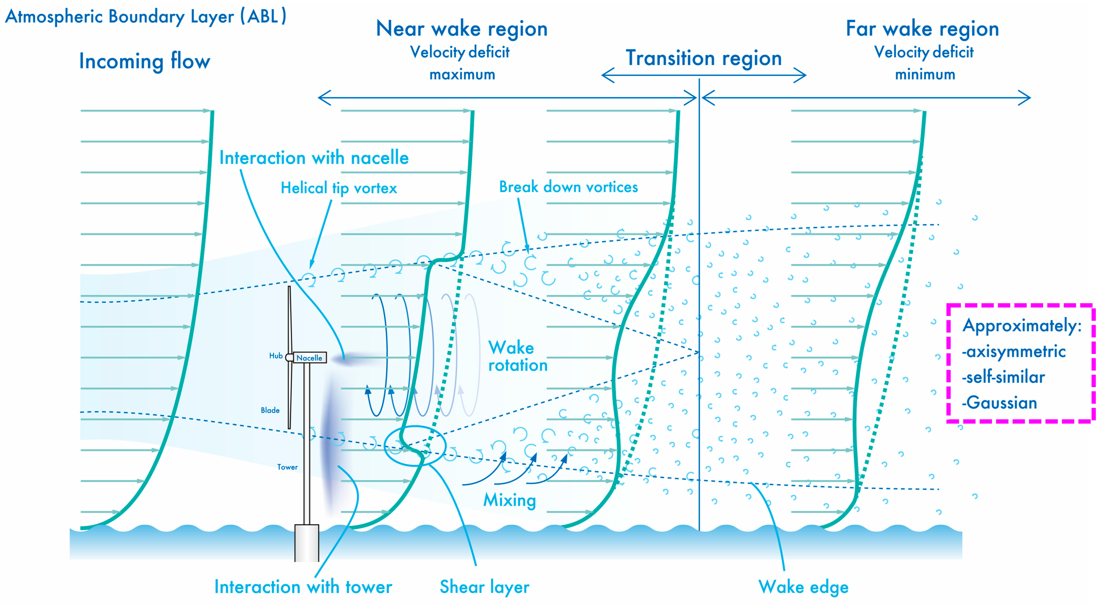
Generally, with the operation of wind turbines, a deficit of wind speed and temporal and spatial fluctuations are formed behind the wind turbines (see Figure 1). These flow phenomena are referred to as wind turbine wakes, and are especially prevalent in large-scale offshore wind farms (WFs) composed of multiple wind turbines, causing a decrease in the power generation of downstream wind turbines. At the same time, these flow phenomena cause failure both inside and outside of the wind turbines. Therefore, it is essential to correctly evaluate the effect of wind turbine wakes formed by upstream wind turbines and to determine the appropriate separation distance between wind turbines. In the evaluation of wind turbine wakes, field measurements and wind tunnel experiments using a scale model are difficult to carry out, so studies based on numerical simulations are generally performed instead [1,2,3,4,5,6]. The method with the highest prediction accuracy is using fully resolved geometries combined with computational fluid dynamics (CFD) simulations [7]. In this method, the structures of the rotating wind turbine blades, nacelle, tower, etc. are modeled in detail by the CFD approach of unsteady Reynolds-averaged Navier–Stokes (RANS) modeling and large-eddy simulation (LES). In these approaches, in order to faithfully reproduce the rotation of the wind turbine blade, special techniques such as the advanced generation of computational grids and a sliding mesh approach are required. For this reason, commercial CFD software is generally used, such as ANSYS(R) Fluent(R), ANSYS(R) CFX(R) [8], and Simcenter STAR-CCM+ [9]. However, these calculations require enormous calculation costs and computer resources and are hardly used for practical wind farm design, which requires the calculation of many wind directions and wind speeds. Recently, the LES approach using a CFD wake model that simulates the rotation of a wind turbine blade based on blade element theory has become a mainstream approach. CFD wake models mainly include actuator disk (AD) models [10], AD models with rotation (ADM-R) [11], actuator line (AL) models [10], and actuator surface (AS) models [12]. However, these approaches require some parameters of the wind turbine-specific blades (i.e., the cord length, twist angle, drag coefficient, and lift coefficient at any cross-sectional position of the blade), and these are often difficult to obtain for wind energy/wind farm developers. As a result, the CFD wake model is currently inconvenient. On the other hand, the engineering wake model (empirical/analytical wake model) represented by the Park model by Jensen [13]/Katic [14] has a very simple series of calculations and is convenient. Therefore, it is still widely used in practical wind farm design in domestic and overseas wind industry. The engineering wake model is a method for predicting wind turbine wakes based on momentum theory, and the flow field is idealized as a precondition for modeling. Therefore, in the case of a large-scale WFs composed of multiple wind turbines, it is difficult to accurately predict the mutual interference of wind turbine wakes, which is a nonlinear flow phenomenon.

Therefore, in the present research, we propose a new LES approach using a porous disk (PD) model as an intermediate method between the engineering wake model (empirical/analytical wake model) and the LES, combined with AD or AL models, especially for the assumption of use in large-scale offshore wind farms (WFs) consisting of multiple wind turbines. In this research, we use the concept of forest canopy model [15,16] as a porous disk (PD) model, which has many research results in the meteorological field. In the forest canopy model, an aerodynamic resistance is added as an external force term to all governing equations (Navier–Stokes equations) in the streamwise, spanwise, and vertical direction. Therefore, like the forest model, the aerodynamic resistance is added to the governing equations in the three directions as an external force term in the porous disk (PD) model. In particular, the main purpose of this approach is to accurately predict the mutual interference of wind turbine wakes, which is a nonlinear flow phenomenon. The CFD porous disk (PD) wake model newly proposed in this research does not cover all wind speed classes from cut-in wind speed to cut-out wind speed of a wind turbine. In the CFD porous disk (PD) wake model proposed in this research, only the wind speed of 10 m/s approaching the hub center of the wind turbine is targeted. In addition, the target wind turbine is only 2-MW. This is because the accurate prediction results of this wind speed class have a very important impact on the evaluation of the feasibility of offshore wind power generation. At the same time, we are focusing on the high-precision prediction of the average loss of the wind velocity component (U-velocity) in the streamwise direction among the three wind velocity components. This is because the wind velocity component (U-velocity) in the streamwise direction has the greatest effect on the evaluation of power generation. Hereinafter, the wind velocity component in the streamwise direction will be denoted by U-velocity.

In order to verify the validity of the new CFD porous disk (PD) wake model proposed in the present study, we compare it with huge computation results using fully resolved geometries combined with unsteady RANS by use of the ANSYS(R) CFX(R) software. As mentioned above, in this research, we attempt to reproduce the wind turbine wake that is formed on the downstream side by the 2-MW wind turbine operating at a wind speed of 10 m/s. Furthermore, in order to verify the prediction accuracy of fully resolved geometries combined with unsteady RANS itself by ANSYS(R) CFX(R), a comparison with wind tunnel experiments using a wind turbine scale model is also performed here.

2. Wind Tunnel Experiment Using a 1/88 Wind Turbine Scale Model and Fully Resolved Geometries Combined with Unsteady RANS by ANSYS(R) CFX(R)

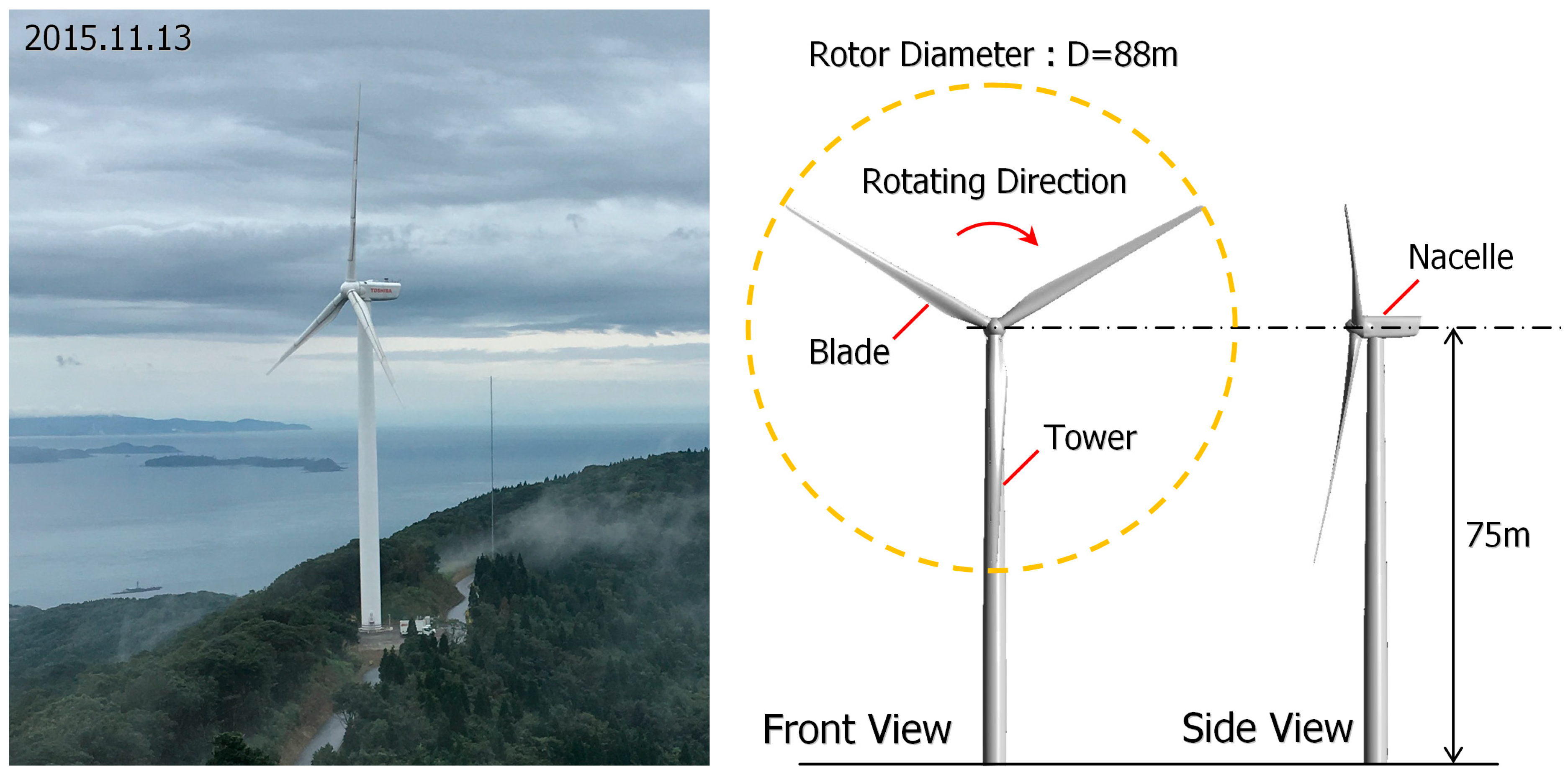
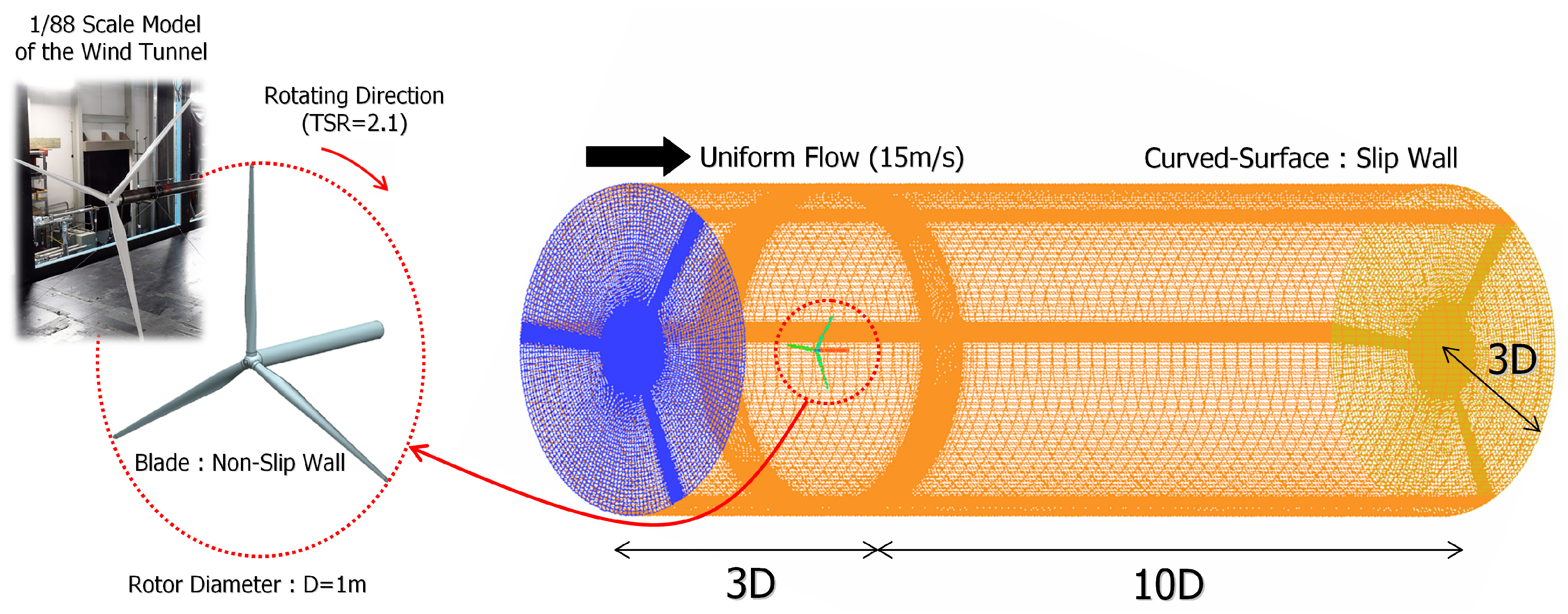
The target wind turbine in the present study is a 2-MW-large wind turbine, shown in Figure 2. In the present study, we propose an LES approach, using a PD model for the purpose of the practical wind farm design of large-scale offshore WFs. First, the prediction accuracy of the fully resolved geometries combined with unsteady RANS is used to verify the validity of the CFD PD wake model. 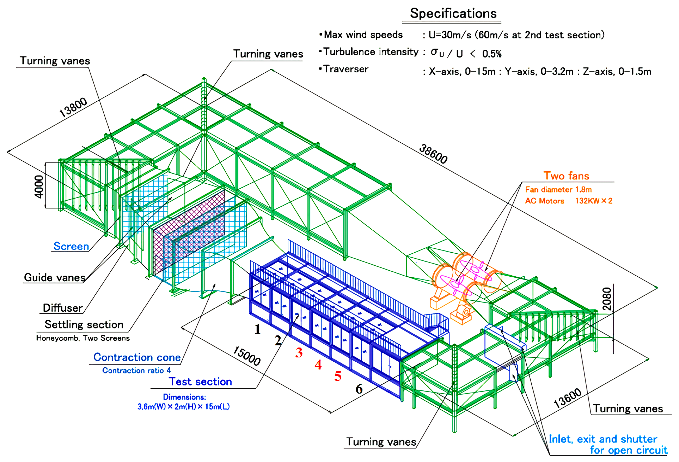The 1/88 scale model (rotor diameter D = 1 m) of a 2-MW wind turbine blade (D = 88 m) shown in Figure 2 was manufactured and a wind tunnel experiment was performed. 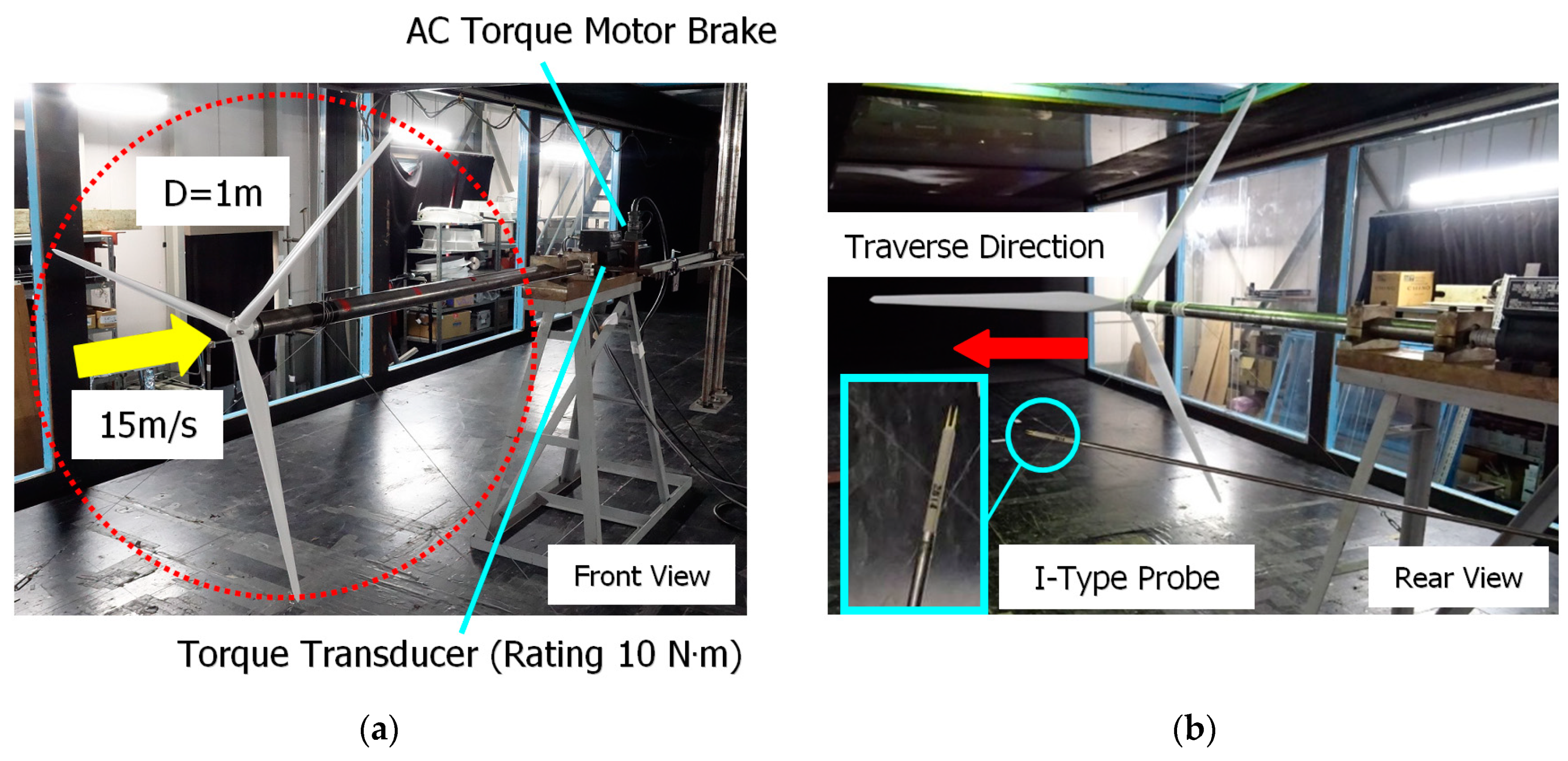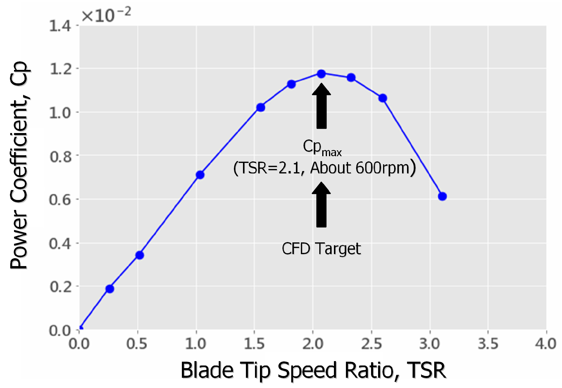The wind tunnel facility used in the present study is a boundary layer wind tunnel (BLWT; 15 m long × 3.6 m wide × 2.0 m high) owned by the Research Institute for Applied Mechanics (RAIM), Kyushu University, shown in Figure 3. As shown in Figure 4, in the wind tunnel experiment, only the blade part was targeted for the scale model. The inflow wind speed was set to 15 m/s, the wind turbine blades were rotated at multiple rotation speeds, and the optimum tip speed ratio (TSR = 2.1, about 600 rpm) at which the power coefficient Cp showed a maximum value was estimated (see Figure 5). The Reynolds number, where the rotor diameter D is defined as the representative length, is of the order of 10⁶.

Then, the wind turbine scale model was rotated at the optimal tip speed ratio (TSR = 2.1) and the velocity distribution was measured by traversing the hot-wire anemometer horizontally in the wake region of the wind turbine. The sampling frequency of the airflow measurement was 1000 Hz, the sampling time was 30 sec, and only the average velocity distribution was evaluated.

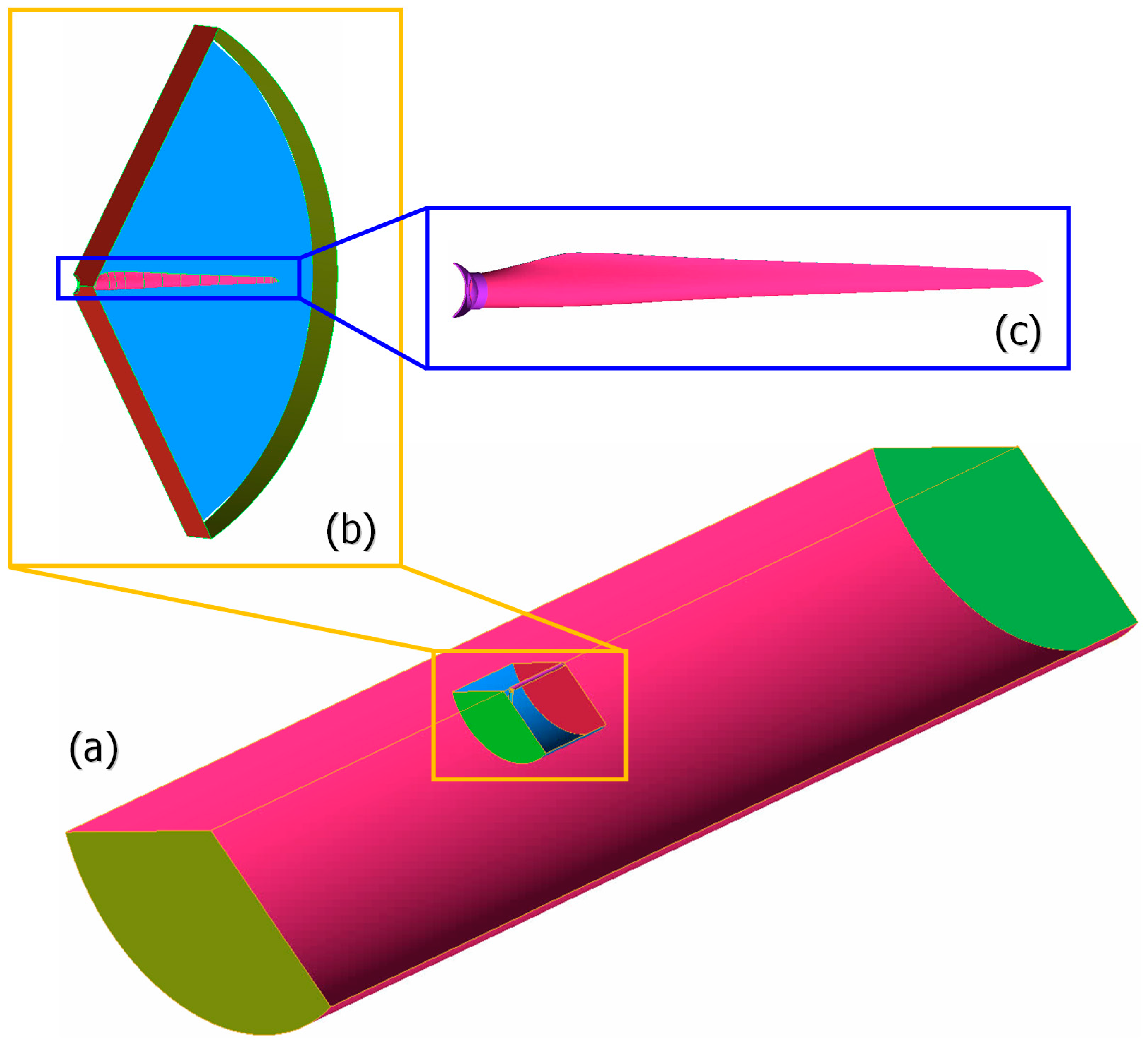
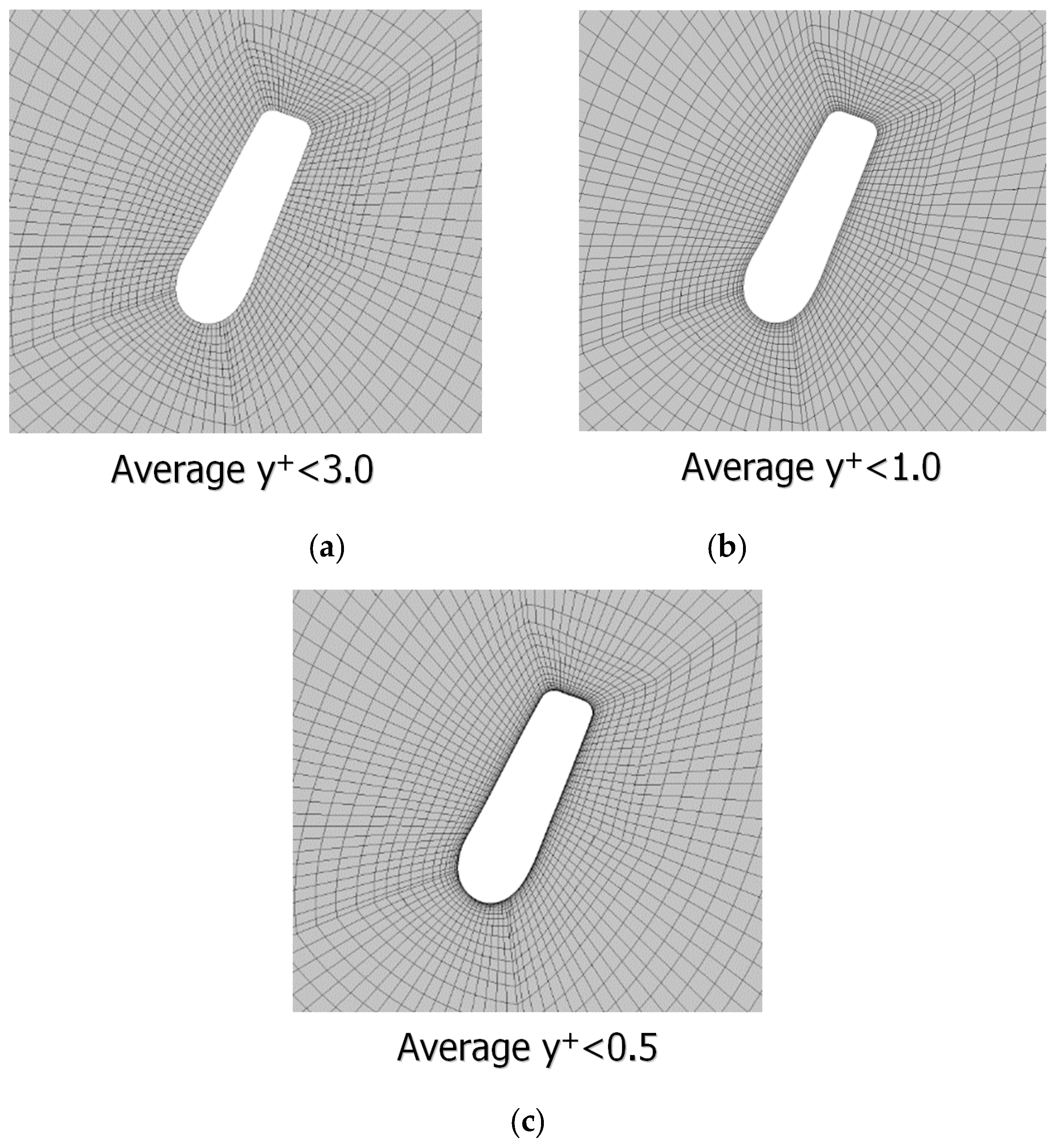
The fully resolved geometries combined with unsteady RANS by ANSYS(R) CFX(R) for a 1/88 scale wind turbine model (rotor diameter D = 1 m) approach was used at the optimum tip speed ratio (TSR = 2.1) estimated by the wind tunnel experiments. As shown in Figure 6 and Figure 7, in the present simulation, the rotating wind turbine blade was faithfully reproduced using the sliding mesh approach. On the other hand, the motor part was not simulated. In the present study, a cylindrical computational grid was set and used. In addition, three types of computational grids were prepared, as shown in Figure 8, to verify the effect of the spatial grid resolution of the blade surface on the flow field. The other simulation conditions are shown in

Table 1. Simulation conditions for the 1/88 scale wind turbine model. RANS: Reynolds-averaged Navier–Stokes.

Pre-Processing (Geometry/Mesh Generation)	ANSYS(R) ICEM CFD(TM) v14.5
Solver	ANSYS(R) CFX(R) v19.3
Turbulence Model	Unsteady RANS (SST k-ω)
Convective Difference Scheme	High Resolution
Number of Meshes	Approximately 15 Million
Time Increment (sec)	1.96e-3 (5 deg/1 step)
Analysis Time (day)	3 (40 Blade Rotations)
Sampling Time (sec)	4.23
Number of Blade Rotations during Sampling	30
Computer Environment	Number of Cores: Total of 1440 cores (60 nodes) Single-node Performance: 24 cores/1 node, Intel Xeon Gold 6136 (3.0 GHz)

.

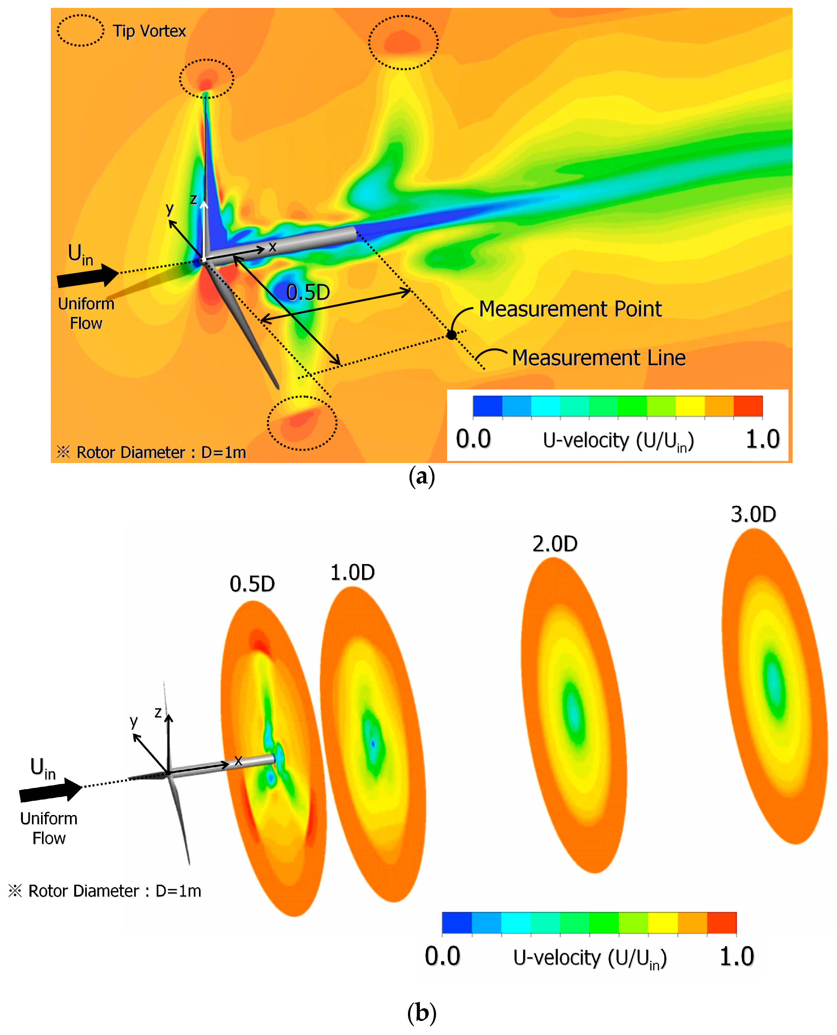
Figure 9 shows the spatial distribution of the velocity components (instantaneous U-velocity) in the streamwise direction for fully resolved geometries combined with unsteady RANS by ANSYS(R) CFX(R) using the standard grid shown in Figure 8b. Looking at Figure 9a, the formation of a tip vortex is clearly observed near the tip of the wind turbine blade. Paying attention to Figure 9b, it can be seen that the velocity deficit region is formed downstream of the wind turbine blade with the rotation of the wind turbine blade. 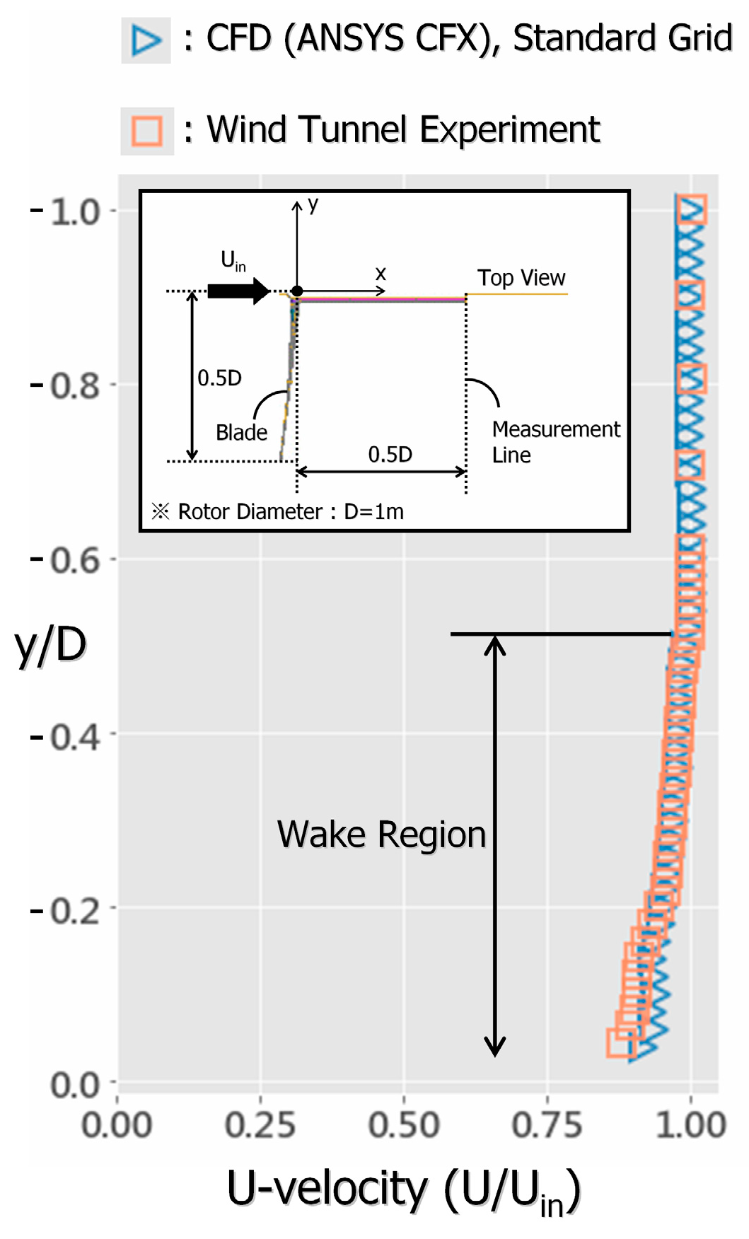Figure 10 shows the comparison of the velocity distribution in the measurement line (x = 0.5D), shown by the dotted line in Figure 9a, with the airflow measurement result by the wind tunnel experiment. Although the description is omitted here for the sake of space, the same tendency was confirmed from the results of the airflow measurement in the wind tunnel experiment using a 1/44 scale wind turbine model (D = 2 m) with twice the blade diameter. The results show that the fully resolved geometries combined with unsteady RANS by ANSYS(R) CFX(R), using the standard grid shown in Figure 8b, are able to reproduce the results of the wind tunnel experiment well.

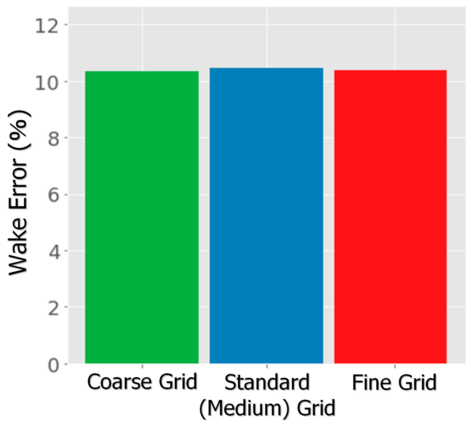
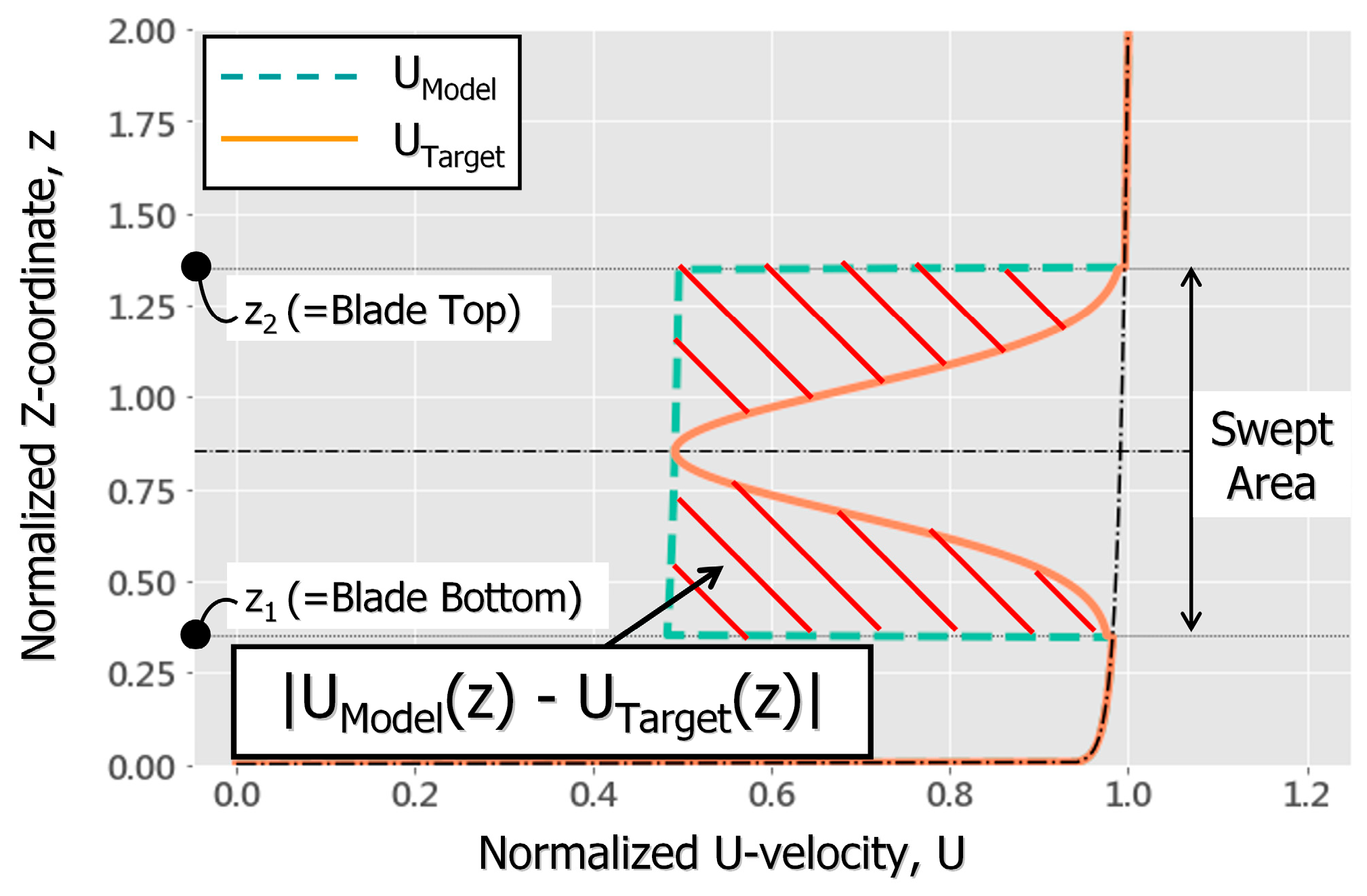
In the present study, the effect of the spatial grid resolution on the wind turbine blade surface on the mean velocity distribution in the wind turbine wake region was verified. For this purpose, we compared the numerical results of three computational grids, as shown in Figure 8. Furthermore, the error rate for the time-averaged wind turbine wake velocity distribution, determined by Figure 11 and Equation (1), is newly defined. The error rate of the time-averaged wind velocity distribution on the measurement line (x = 0.5D), shown by the dotted line in Figure 9a, was evaluated with respect to the wind tunnel experiment results. Figure 12 shows the obtained numerical results. As shown in Figure 12, the error rate of the calculation results by ANSYS(R) CFX(R), with respect to the wind tunnel test results, was about 10% for all three types of computational grids used.

$$\mathrm{W}\mathrm{a}\mathrm{k}\mathrm{e} \mathrm{E}\mathrm{r}\mathrm{r}\mathrm{o}\mathrm{r} (\%)={\displaystyle {\int }_{{\mathrm{z}}_1}^{{\mathrm{z}}_2}\frac{\left|{\mathrm{U}}_{\mathrm{M}\mathrm{o}\mathrm{d}\mathrm{e}\mathrm{l}}\left(\mathrm{z}\right)-{\mathrm{U}}_{\mathrm{Target}}\left(\mathrm{z}\right)\right|}{{\mathrm{U}}_{\mathrm{Target}}\left(\mathrm{z}\right)} }\mathrm{d}\mathrm{z} \times 100$$

(1)

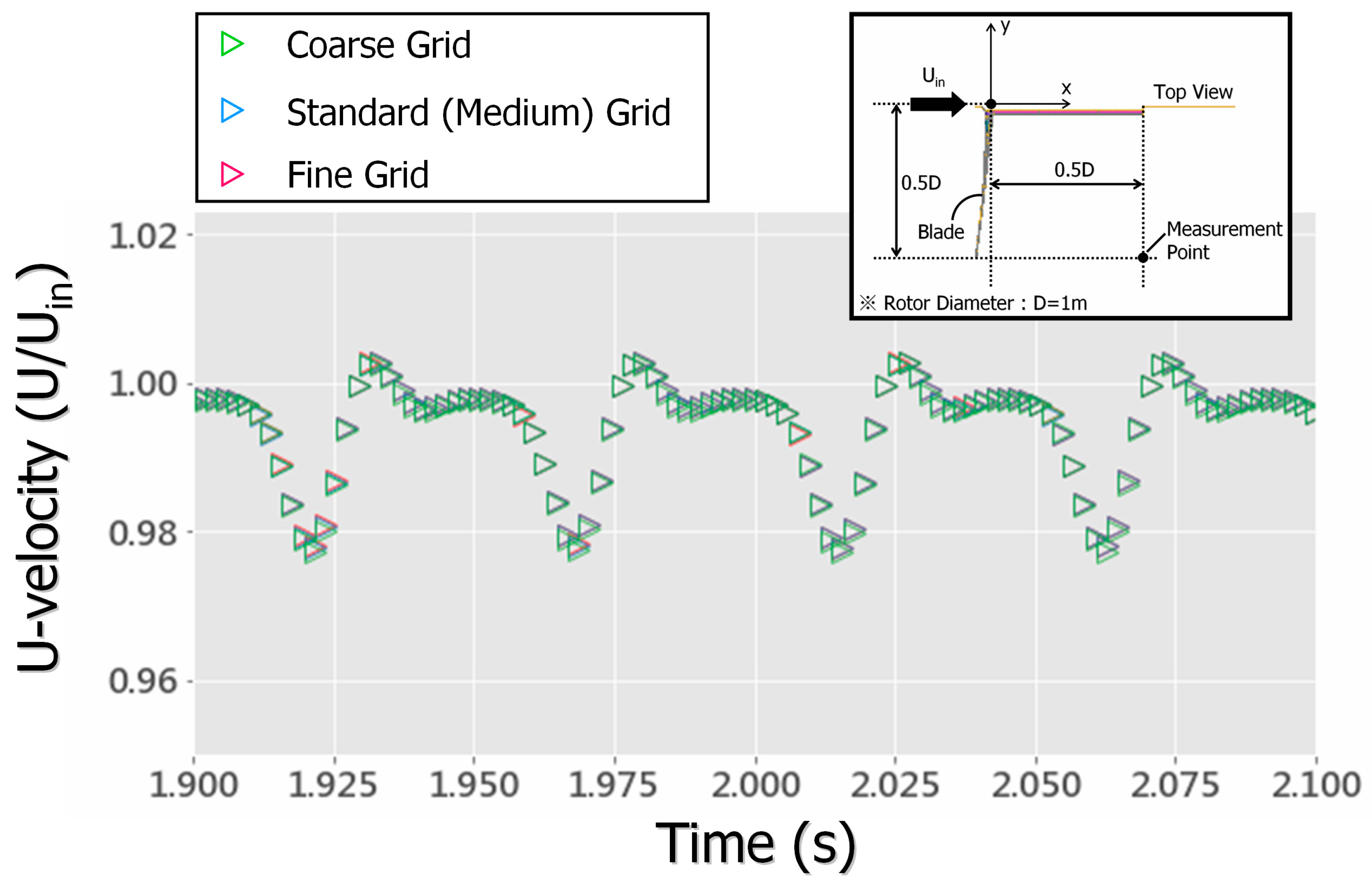
As described in Figure 9, near the tip of the wind turbine blade, a tip vortex is formed downstream of the wind turbine as the blade passes. In the present study, we also examined the effect of the difference in the spatial grid resolution on the wind turbine blade surface on the shedding period of the tip vortex. Figure 13 shows the comparison of the time change of instantaneous U-velocity at the measurement point (x = 0.5D, y = −0.5D), indicated by the black circle symbol. The observation of this figure shows that periodic velocity fluctuations appear with the formation of the tip vortex. In addition, no significant differences were found in the numerical results of the three different spatial grid resolutions studied in the numerical study, and almost the same results were obtained.

From the above, in the present study, it was confirmed that the difference in the spatial grid resolution of the wind turbine blade surface had little effect on the prediction accuracy of the airflow characteristics in the wind turbine wake region. Accordingly, within the range of the spatial grid resolution set in the present study, it was judged that the fully resolved geometries combined with Unsteady RANS approach, determined using ANSYS(R) CFX(R), could properly reproduce the flow phenomena in the wind tunnel experiment when using the wind turbine scale model.

3. Fully Resolved Geometries Combined with Unsteady RANS, Calculated by ANSYS(R) CFX(R) for a Real Wind Turbine

Due to temporal and spatial limitations, it is difficult to perform a comprehensive field measurement of wind turbine wakes using real wind turbines. Therefore, a time-averaged wind speed database in the wind turbine wake region was created with the fully resolved geometries combined with Unsteady RANS approach by ANSYS(R) CFX(R). The CFD porous disk (PD) wake model that is newly proposed in the present study was verified based on the obtained time-averaged wind speed database. This section describes the details of the new approach for a real wind turbine. In the present study, we consider the situation where a 2-MW class wind turbine (rotor diameter D = 88 m and wind turbine hub height of 75 m), shown in Figure 2, is installed on ideal flat terrain. Figure 14 shows the computational domain and computational grid for the real wind turbine. As in the case of the 1/88 scale wind turbine model shown above, the blade part used a sliding mesh approach, and the wind turbine blade was rotated at a rotation speed of 5 deg in one step for the simulation. The TSR set in the present simulation was of the optimum value of 5.87 at a wind speed of 10 m/s. The thrust coefficient Ct at that time was about 0.8. In this simulation, the nacelle and the tower were modeled in detail. The spatial grid resolution of the wind turbine blade surface was set to y⁺ = 2.3 based on the numerical results in described in Chapter 2. The inflow wind speed distribution followed the power law velocity profile, where N = 10, and the wind speed at the hub center of the wind turbine was 10 m/s. Here, the wind speed of 10 m/s corresponds to the vicinity of the maximum value of the power coefficient Cp. The k-ω SST model (unsteady RANS) was adopted as the turbulence model, the same as in the simulation in Chapter 2. The other simulation conditions were as shown in

Table 2. Simulation conditions for the real wind turbine.

Pre-Processing (Geometry/Mesh Generation)	ANSYS(R) ICEM CFD(TM) v14.5
Solver	ANSYS(R) CFX(R) v19.3
Turbulence Model	Unsteady RANS (SST k-ω)
Convective Difference Scheme	High Resolution
Number of Meshes	Approximately 14 Million
Time Increment (sec)	5.45e-2 (5 deg/1 step)
Analysis Time (day)	10 (140 Blade Rotations)
Sampling Time (sec)	117.65
Number of Blade Rotations during Sampling	30
Computer Environment	Number of Cores: Total of 1440 cores (60 nodes) Single-node Performance: 24 cores/1 node, Intel Xeon Gold 6136 (3.0 GHz)

.

Figure 15 shows the simulation results (spatial distribution of instantaneous U-velocity) for the real wind turbine considered here. Paying attention to the side view shown in Figure 15a, it can be seen that the velocity deficit region is clearly formed downstream of the wind turbine. Flow separation occurs at the root of the wind turbine blade, resulting in large fluid resistance near the hub center of the wind turbine. Furthermore, near the wind turbine nacelle, the fluid passing through the wind turbine blade locally increases in speed. Focusing on the front view of x = 5D of the near wake region shown in Figure 15b and x = 10D of the far wake region shown in Figure 15c, it can be seen that the concentric wind turbine wake region gradually diffuses outward as the separation distance from the wind turbine increases.

4. Large-Eddy Simulation Using the Porous Disk Model Approach for Real Wind Turbines

In the present study, in order to support the practical wind farm design for wind energy/wind farm developers, we propose a new LES method using the porous disk (PD) wake model approach as an intermediate method between the engineering wake model (empirical/analytical wake model) and the LES combined with AD or AL models. This method assumes the use of a large-scale offshore wind farm (WF) with multiple wind turbines. Furthermore, we aimed for the accurate prediction of the complicated mean wind speed distribution formed by the mutual interference of wind turbine wakes. For this purpose, as the first step, we focused only on the wind speed of 10 m/s approaching the hub center of the wind turbine, which has the greatest impact on the evaluation of practical wind farm design.

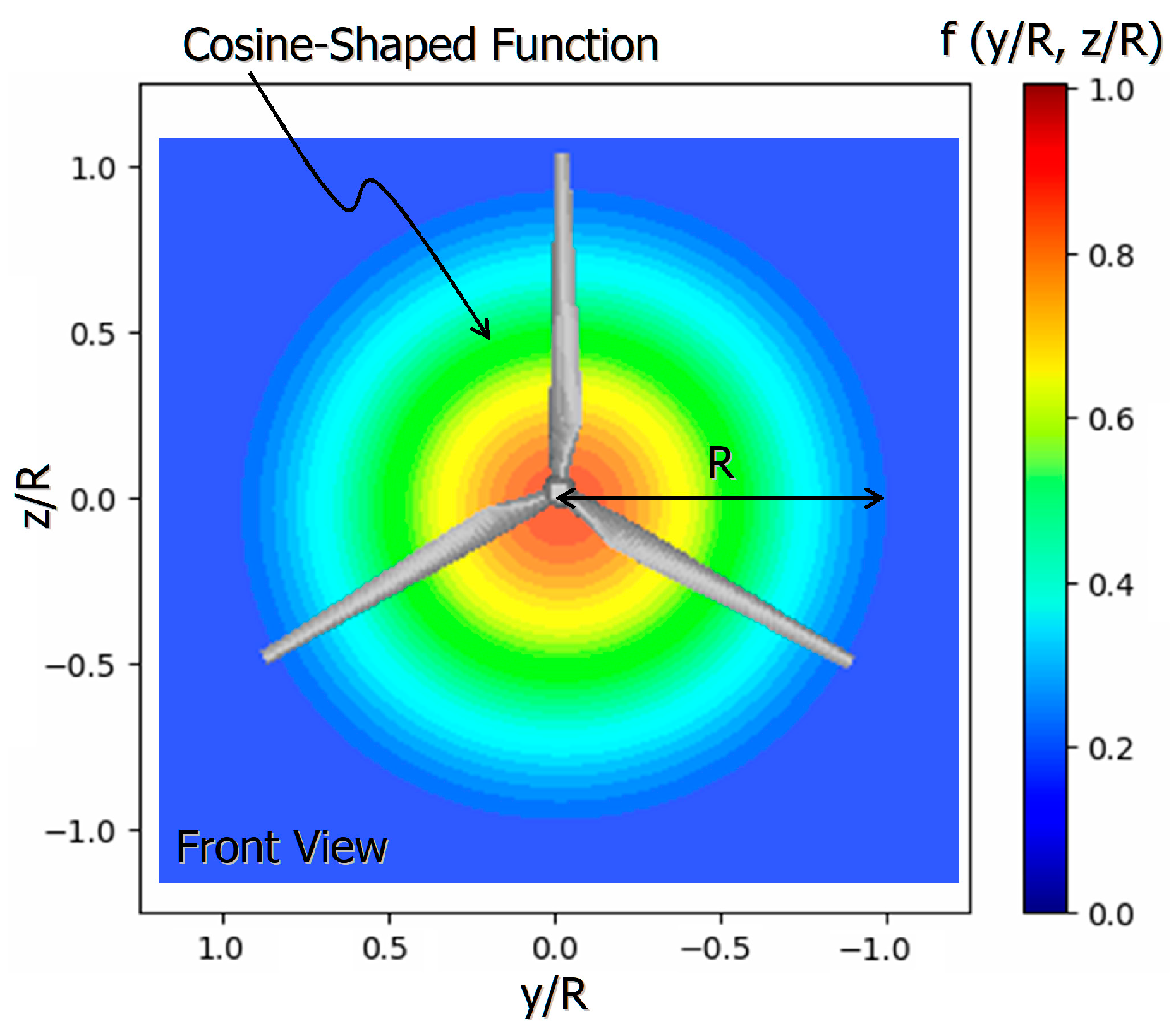
This section describes the concept of the CFD PD wake model that is proposed in the present study. As mentioned earlier, in this research, we first use the concept of forest canopy model as a porous disk (PD) model, which has many research results in the meteorological field. In the forest canopy model, an aerodynamic resistance is added as an external force term to all governing equations (Navier–Stokes equations) in the streamwise, spanwise, and vertical direction. Therefore, like the forest model, the aerodynamic resistance is added to the governing equations in the three directions as an external force term in the porous disk (PD) model (see Equation (3)). Here again, we pay attention to the part surrounded by the purple dotted line shown in Figure 1. The words in the part surrounded by the purple dotted line are very important keywords. Next, we consider that the vertical shape of the wind velocity distribution in the wake flows formed downstream of the wind turbine has a strong correlation with the vertical shape of the aerodynamic resistance in the swept area of the wind turbine. Based on the above two concepts, the swept area of the wind turbine is expressed as a disk-shaped resistor with a thickness in the streamwise direction as a porous disk (PD), where the difference in fluid (aerodynamic) resistance was reproduced using a new model parameter C_RC (the drag coefficient) instead of the thrust coefficient Ct. Furthermore, the spatial distribution was given in the swept area by multiplying the model parameter C_RC by the cosine-shaped distribution function shown in Figure 16. In the swept area, the model parameter C_RC, as a resistance value, reaches a maximum at the hub center of the wind turbine, and its value becomes the minimum (zero) toward the tip of the wind turbine blade. In order to verify the validity of the CFD PD wake model proposed in the present study and to determine the optimal value of the model parameter C_RC, a comparison was made with the fully resolved geometries combined with unsteady RANS approach by ANSYS(R) CFX(R), described in Chapter 3.

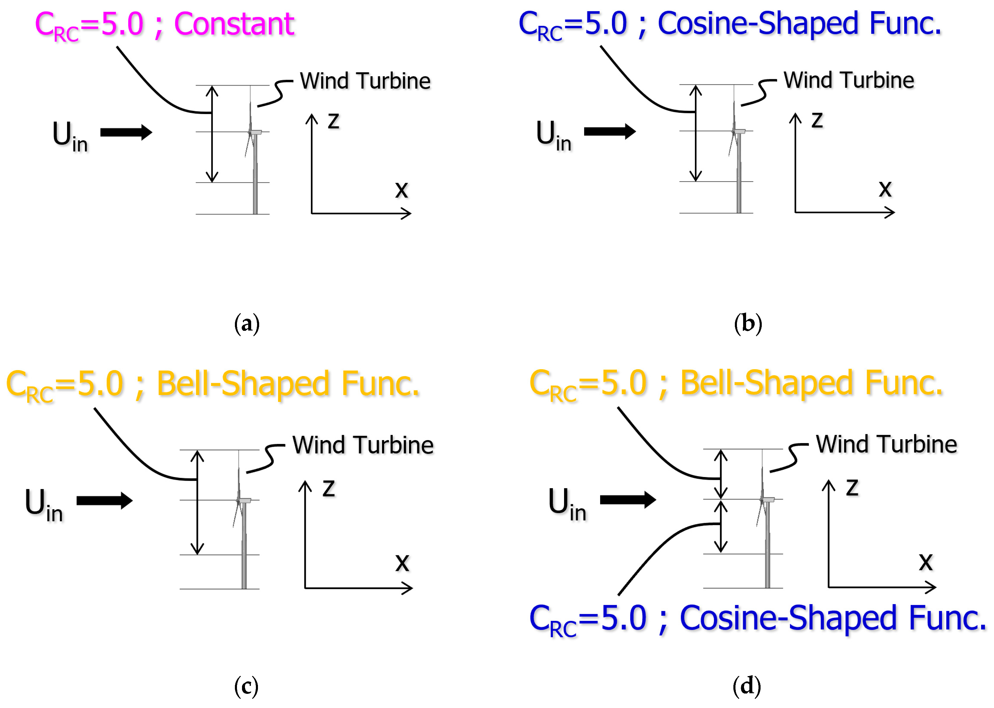
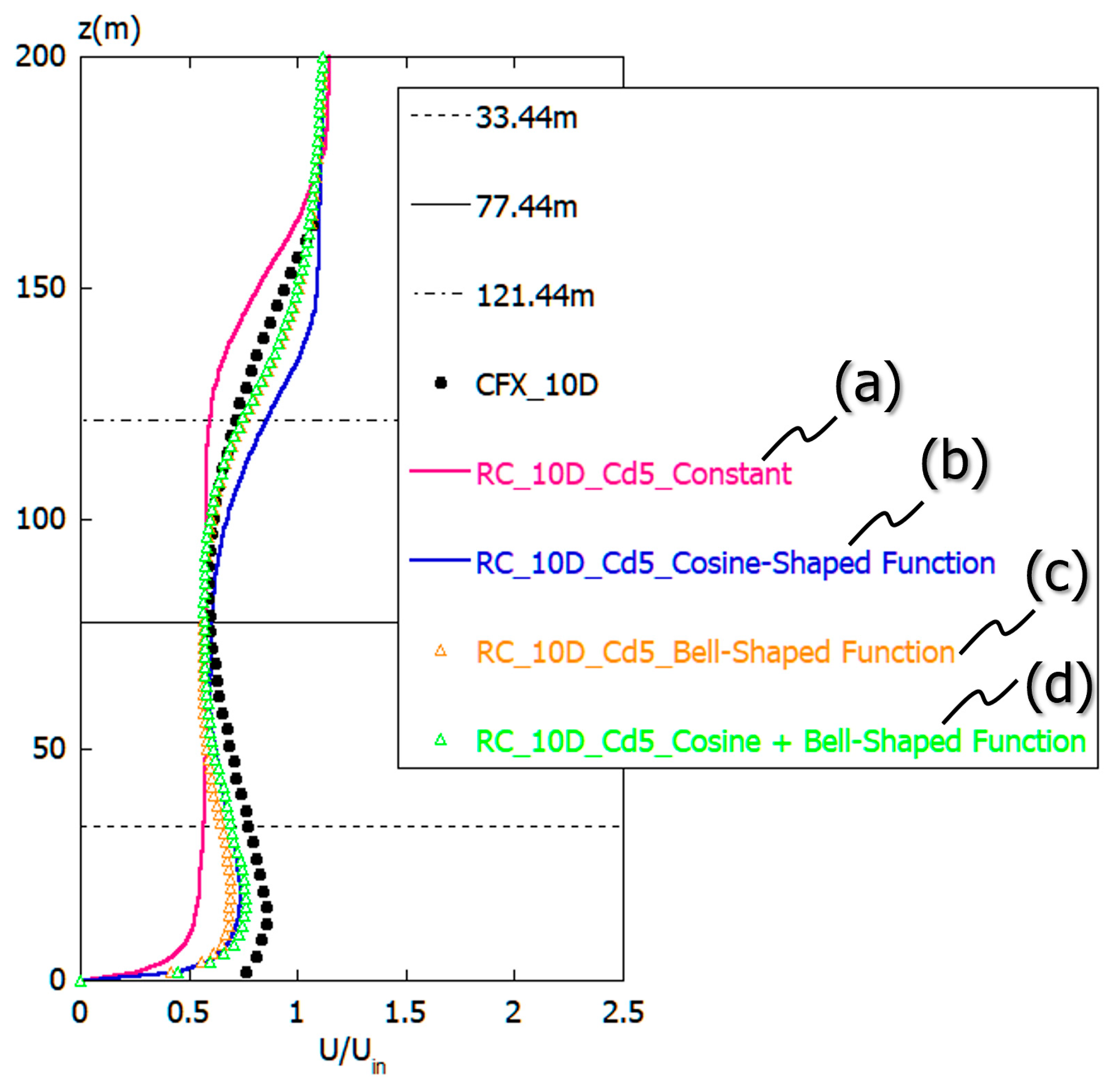
The point to be emphasized here is that there is a strong correlation between the vertical velocity distribution in the wind turbine wake and the distribution of the model parameter C_RC of the CFD PD wake model set in the swept area of wind turbine. Based on this assumption, the spatial distribution in the swept area of the wind turbine was determined by multiplying the parameter C_RC by the correction function such as cosine-shaped distribution function. That is, the C_RC is not set to a constant value in the swept area of the wind turbine. The spatial distribution of C_RC is gradually changed from the center of the wind turbine to the tip using a correction function. This is based on the physical consideration of the flow characteristics in the wind turbine wake region (results of the wind tunnel experiment conducted in this study and past research results [17]). This is also a novel idea in this research that has never existed before. Furthermore, the correction function is not limited to the cosine-shaped distribution function (see Appendix A). For example, by using a Gaussian function or a spline function to modify the model parameter C_RC distribution of the CFD PD wake model in the swept area of wind turbine more precisely, the amount of wind velocity (U-velocity) loss in the streamwise direction can be further improved. In the future, we plan to further study how to give the spatial distribution of C_RC for a wide range of wind speed classes and different wind turbine sizes including large offshore wind turbines of 10 MW or higher power levels.

In the optimization of the model parameters, it is necessary to quantify how correctly the flow characteristics in the wind turbine wake can be evaluated. Generally, the wind speed at the hub center of the wind turbine is used as the representative wind speed for the evaluation of power generation. However, the wind speed at the hub center of the wind turbine cannot be said to be a representative wind speed in recent years, where efficiency has increased due to the increase in size of wind turbines. Recently, an example using the rotor equivalent wind speed (REWS) was reported, considering the wind speed distribution in the swept area as a representative wind speed [18]. Therefore, in the present study, as shown in Equation (1), the difference between the target wind speed and the predicted wind speed in the wind turbine wake (red hatching shown in Figure 11) was integrated in the vertical range of the swept area, and this value was newly defined as the wake error. The optimal value of C_RC, which is the only model parameter in the CFD PD wake model, was determined by conducting a parameter survey so that the wake error defined in Equation (1) was minimized. For the target wind speed shown in Equation (1), the huge computation results of the fully resolved geometries combined with unsteady RANS by ANSYS(R) CFX(R), described in Chapter 3 (time-averaged wind speed database in the wind turbine wake region), were used.

In this research, we used a real urban version from RIAM-COMPACT (Research Institute for Applied Mechanics, Kyushu University, Computational Prediction of Airflow over Complex Terrain) based on non-uniform staggered Cartesian grids [19,20,21]. In the staggered Cartesian grid system, the physical velocity components multiplied by the Jacobian are staggered with respect to the pressure, which is placed in the center of the cells. The numerical calculation method is based on the finite-difference method (FDM) and incorporates LES into the turbulence model. In LES, a spatial filter is set up in the flow field, and large- and small-sized turbulent eddies are separated into those with a grid scale (GS) component larger than the computational grid and those with a sub-grid scale (SGS) component, which is smaller. The turbulent eddies with large GS components are directly applied in numerical simulation, independent of the model. The energy dissipative action due to the turbulent eddies with a small GS component is modeled based on physical consideration of SGS stress.

We applied a continuous equation of incompressible fluid with a filter operation (Equation (2)) and the Navier–Stokes equation (Equation (3)) in the dominant flow equations. The computational algorithm was based on the fractional step (FS) method [22], and the time marching method was based upon Euler’s explicit scheme. Poisson’s equation of pressure was solved by successive over-relaxation (SOR). The second-order accurate central-difference scheme was used for the discretization of all spatial terms, excluding the convective term of Equation (3), where the third-order upwind differencing scheme was used for convective terms. An interpolation method [23] was used for the fourth-order accurate central-difference scheme, constituting convective terms. The weight of the numerical dispersion terms of the third-order upwind differencing scheme was presumed to be α = 0.3 against the α = 0.5 value of the Kawamura–Kuwahara scheme [24], and its effect was sufficiently small on the numerical results. A mixed time scale (MTS) model [25] was used for the SGS model of LES (Equations (6)–(13)). The effect of the porous disk was implemented as an external force using Equations (4) and (5). The only parameter of the porous disk model, C_RC, is the resistance coefficient, and we used 5, 6, 7, 8, 9, and 10 for it (C_RC). The RANS results and the present LES results were compared in the latest findings [26], and the prediction accuracy of the present LES approach by comparison with wind tunnel experiments was discussed [27].

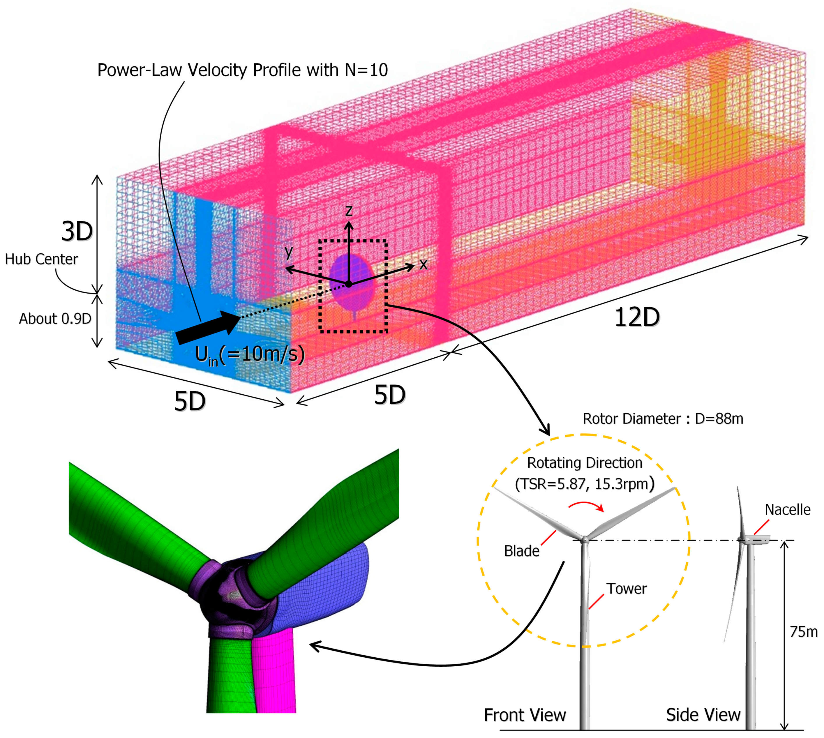
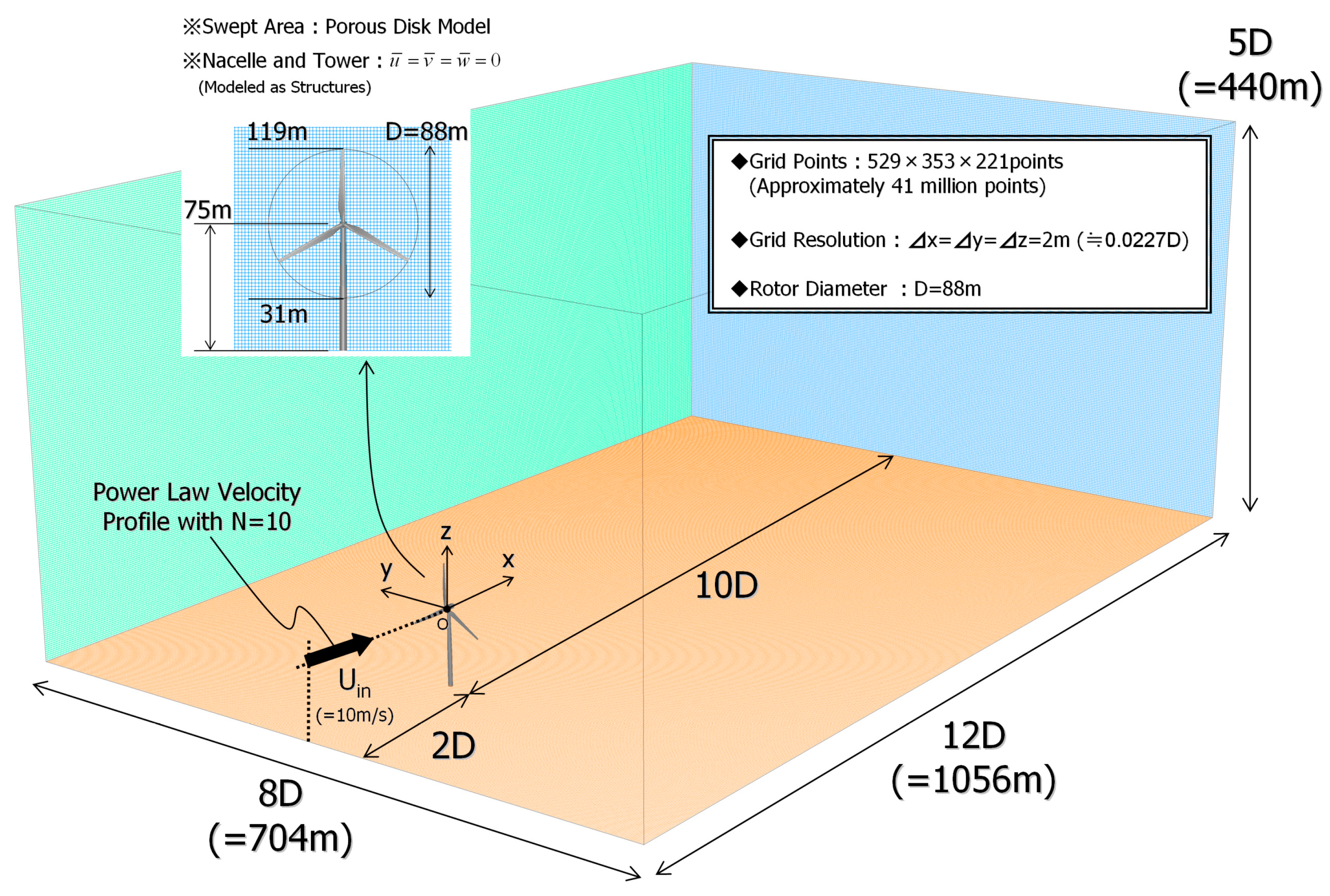
The calculation domain and computational grid are shown in Figure 17. The calculation areas had a space of 1056 (x) × 704 (y) × 440 (z) m in the streamwise (x), spanwise (y), and vertical directions (z), respectively. The grid resolution in all directions was 2 m. Therefore, the number of grids was approximately 41 million points. The present calculation was performed under almost the same conditions as the calculation described in Chapter 3. Concerning the boundary conditions, the power law distribution following N = 10, shown in Figure 18, was assigned to inflow conditions. The lateral interfaces and upper interface were assigned a slip condition and the outflow interface was assigned a convection-type outflow condition. A no-slip condition was assigned to the surface of the ground. The time step was set to Δt = 5 × 10^–4 D/U_in, where D represents the rotor diameter.

$$\frac{\partial {\mathrm{u}}_{\mathrm{i}}}{\partial {\mathrm{x}}_{\mathrm{i}}}=0$$

(2)

$$\frac{\partial {\mathrm{u}}_{\mathrm{i}}}{\partial \mathrm{t}}+{\mathrm{u}}_{\mathrm{j}}\frac{\partial {\mathrm{u}}_{\mathrm{i}}}{\partial {\mathrm{x}}_{\mathrm{j}}}=-\frac{\partial \mathrm{p}}{\partial {\mathrm{x}}_{\mathrm{i}}}+\frac{1}{\mathrm{Re}}\frac{{\partial }^2{\mathrm{u}}_{\mathrm{i}}}{\partial {\mathrm{x}}_{\mathrm{j}}\partial {\mathrm{x}}_{\mathrm{j}}}$$

(3)

$${\mathrm{F}}_{\mathrm{i}}={\mathrm{C}}_{\mathrm{R}\mathrm{C}}\cdot \mathrm{f}\left(\mathrm{y}/\mathrm{R},\mathrm{z}/\mathrm{R},\right)\cdot {\overline{\mathrm{u}}}_{\mathrm{i}}\cdot \mathrm{V}$$

(4)

$$\mathrm{V}=\sqrt{{\overline{\mathrm{u}}}^2+{\overline{\mathrm{v}}}^2+{\overline{\mathrm{w}}}^2}$$

(5)

$${\mathsf{\tau }}_{\mathrm{i}\mathrm{j}}\approx \overline{{\mathrm{u}}_{{}_{\mathrm{i}}}^{\prime }{\mathrm{u}}_{{}_{\mathrm{j}}}^{\prime }}\approx \frac{1}{3}\overline{{\mathrm{u}}_{\mathrm{k}}^{\prime }{\mathrm{u}}_{\mathrm{k}}^{\prime }}{\mathsf{\delta }}_{\mathrm{i}\mathrm{j}}-2{\mathsf{\nu }}_{\mathrm{S}\mathrm{G}\mathrm{S}}{\overline{\mathrm{S}}}_{\mathrm{i}\mathrm{j}}$$

(6)

$${\mathsf{\nu }}_{\mathrm{S}\mathrm{G}\mathrm{S}}={\mathrm{C}}_{\mathrm{M}\mathrm{T}\mathrm{S}}{\mathrm{k}}_{\mathrm{e}\mathrm{s}}{\mathrm{T}}_{\mathrm{S}}$$

(7)

$${\mathrm{C}}_{\mathrm{M}\mathrm{T}\mathrm{S}}=0.05$$

(8)

$${\mathrm{k}}_{\mathrm{e}\mathrm{s}}={({\overline{\mathrm{u}}}_{\mathrm{k}}-{\widehat{\overline{\mathrm{u}}}}_{\mathrm{k}})}^2$$

(9)

$${\mathrm{T}}_{\mathrm{S}}{}^{-1}={\left(\frac{\Delta }{\sqrt{{\mathrm{k}}_{\mathrm{e}\mathrm{s}}}}\right)}^{-1}+{\left(\frac{{\mathrm{C}}_{\mathrm{T}}}{\left|{\overline{\mathrm{S}}}_{\mathrm{i}\mathrm{j}}\right|}\right)}^{-1}$$

(10)

$$\left|{\overline{\mathrm{S}}}_{\mathrm{i}\mathrm{j}}\right|={\left(2{\overline{\mathrm{S}}}_{\mathrm{i}\mathrm{j}}{\overline{\mathrm{S}}}_{\mathrm{i}\mathrm{j}}\right)}^{1/2}$$

(11)

$${\overline{\mathrm{S}}}_{\mathrm{i}\mathrm{j}}=\frac{1}{2}\left(\frac{\partial {\overline{\mathrm{u}}}_{\mathrm{i}}}{\partial {\mathrm{x}}_{\mathrm{j}}}+\frac{\partial {\overline{\mathrm{u}}}_{\mathrm{j}}}{\partial {\mathrm{x}}_{\mathrm{i}}}\right)$$

(12)

$${\mathrm{C}}_{\mathrm{T}}=10.0$$

(13)

$$\Delta ={\left({\Delta }_{\mathrm{x}}\cdot {\Delta }_{\mathrm{y}}\cdot {\Delta }_{\mathrm{z}}\right)}^{1/3}$$

(14)

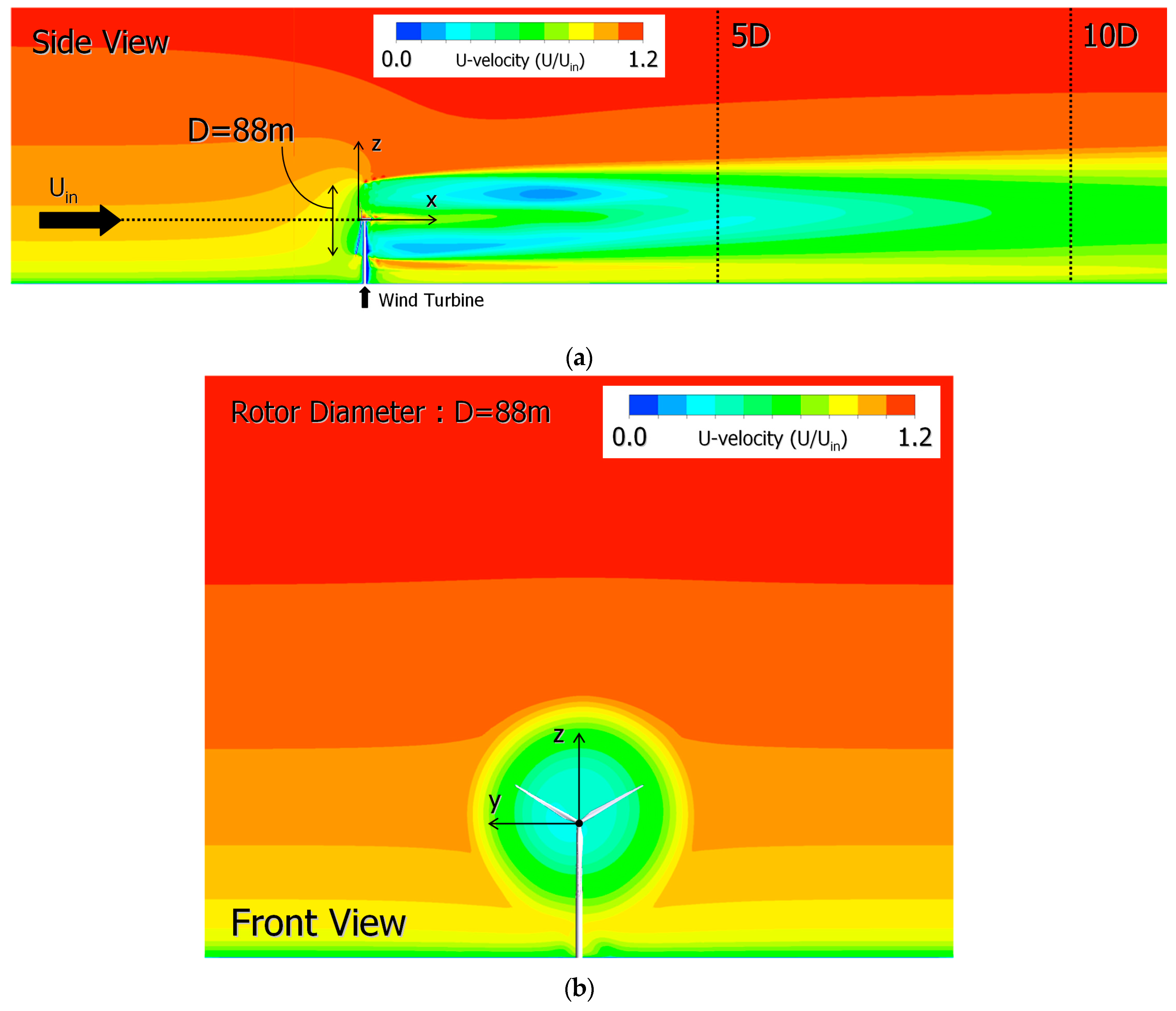
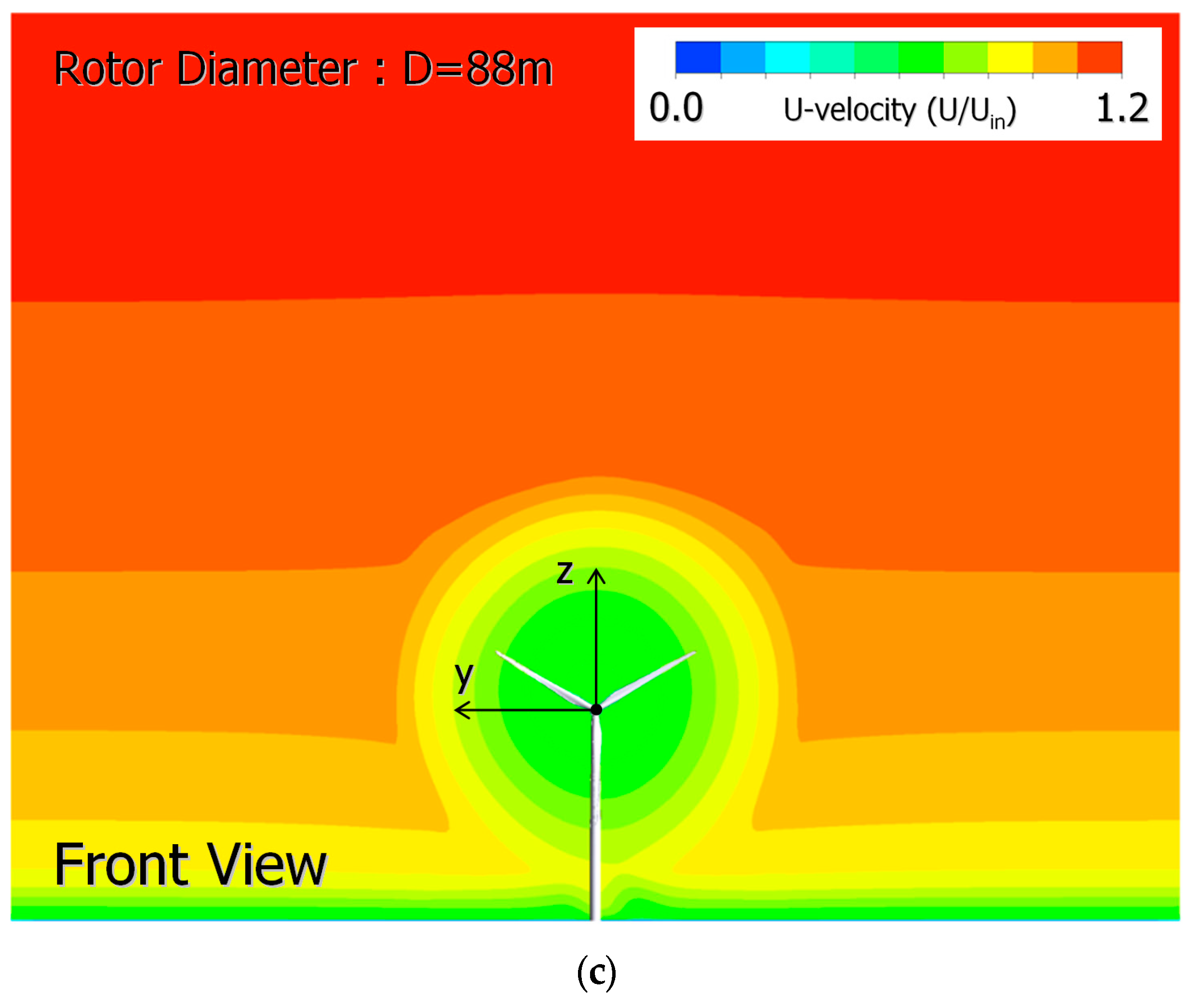
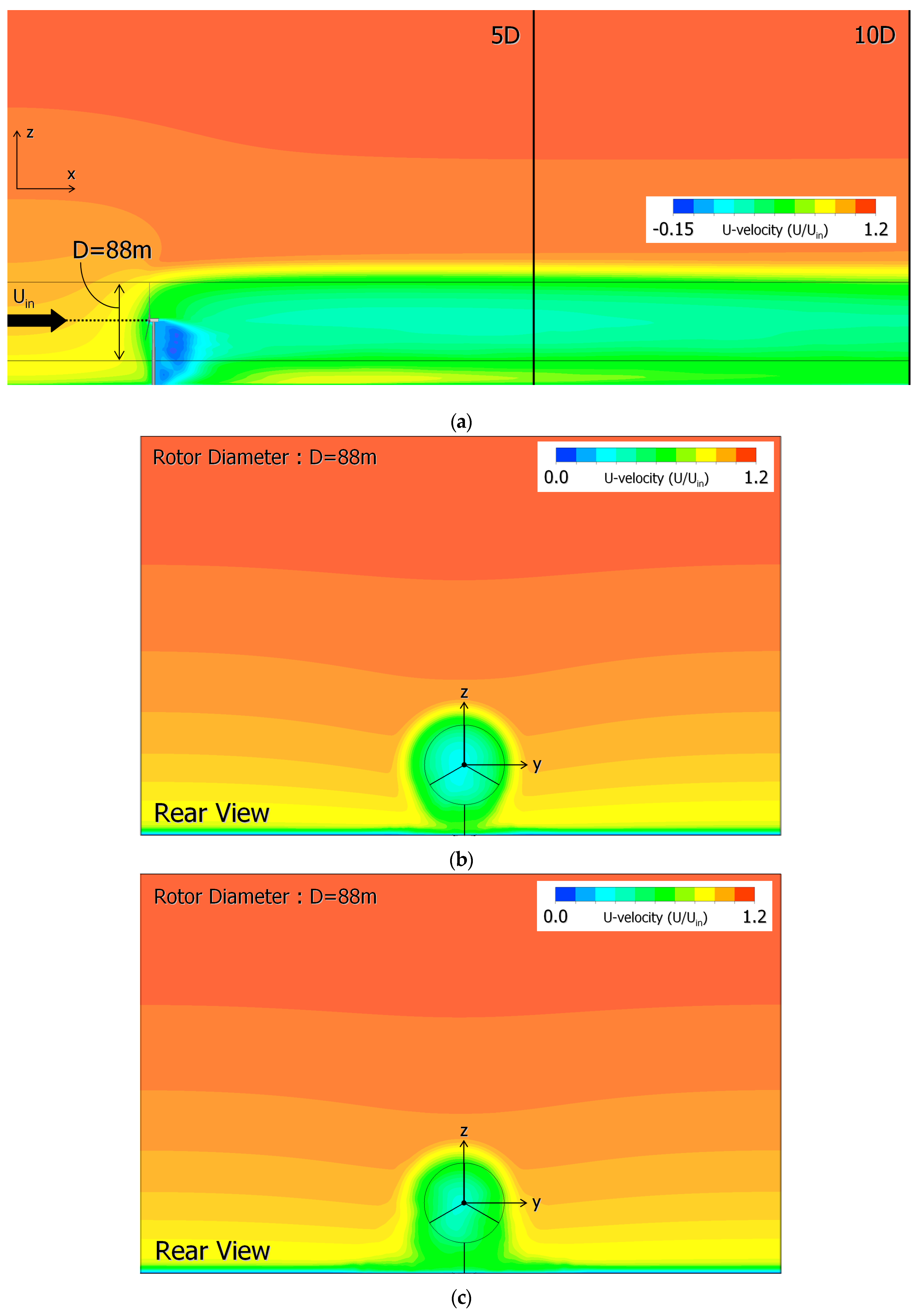
Figure 18 shows the spatial distribution of the velocity component (time-averaged U-velocity) in the streamwise direction in the time-averaged flow field. Looking at the side view shown in Figure 18a, it can be seen that the velocity deficit region is clearly formed downstream of the wind turbine. Looking at the rear view shown in Figure 18b,c, it can be seen that the concentric wake region gradually diffuses outward as the distance from the wind turbine increases. Comparing these simulation results with those for the real wind turbine by ANSYS(R) CFX(R), shown in Figure 15a, it became clear that almost the same tendency of the flow pattern was obtained.

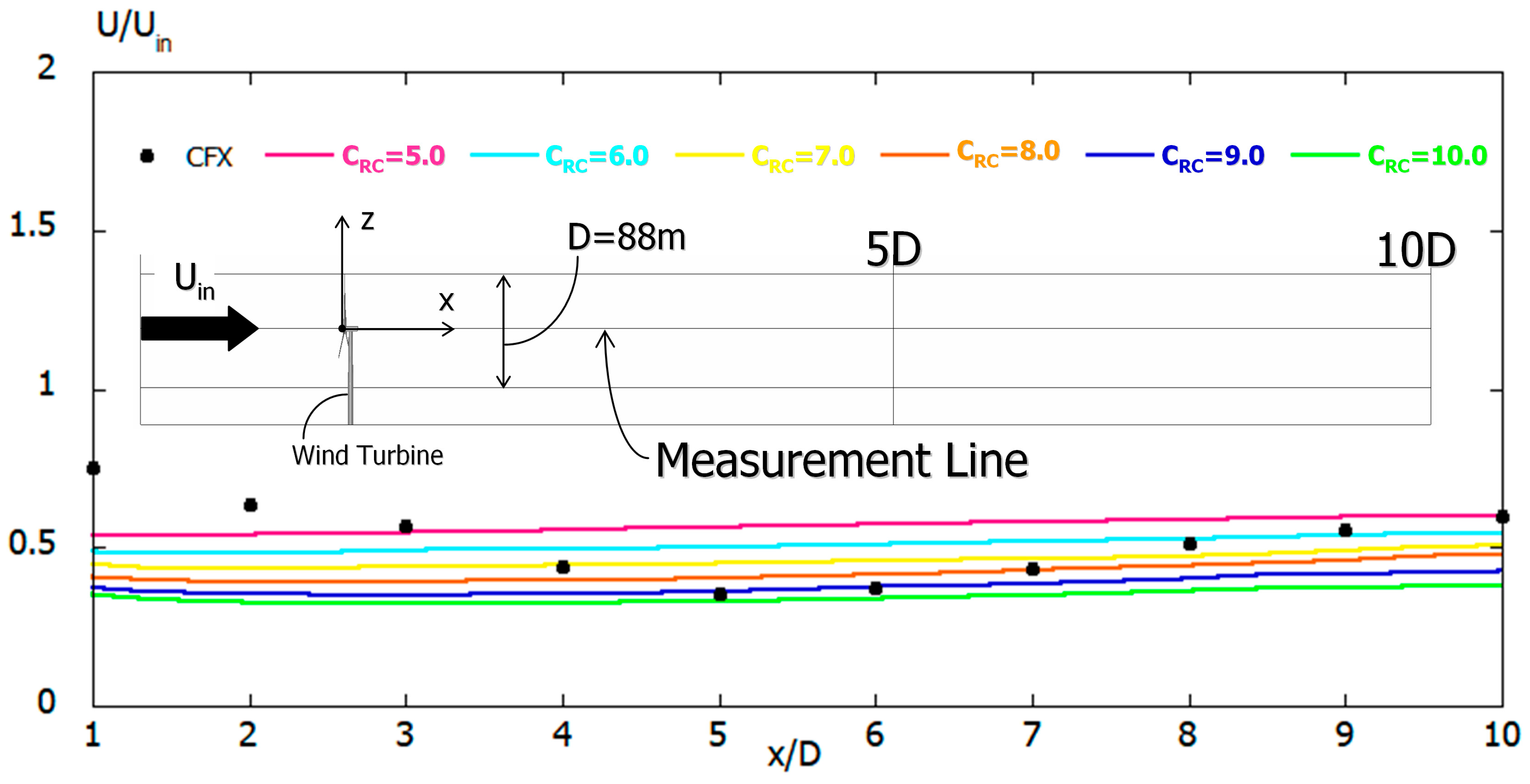
Figure 19 shows the spatial distribution of time-averaged U-velocity at the hub center of the wind turbine with respect to the time-averaged flow field. It should be noted here that in the range from x = 5D of the near wake region to x = 10D of the far wake region, the simulation results for the real wind turbine by ANSYS(R) CFX(R) are in the range of the CFD PD wake model results (C_RC = 5.0 to 10.0) from the newly proposed method in the present study. In other words, in the range of x = 5D of the near wake region to x = 10D of the far wake region, this suggests that wind energy/wind farm developers can accurately evaluate the average velocity deficit at the separation distance by selecting the model parameter C_RC corresponding to the required separation distance. For example, if wind energy/wind farm developers want to know the exact time-averaged velocity deficit at x = 5D, they should set C_RC to 9.0 or 10.0, or if they want to know the exact time-averaged velocity deficit at x = 10D, they should set C_RC to 5.0.

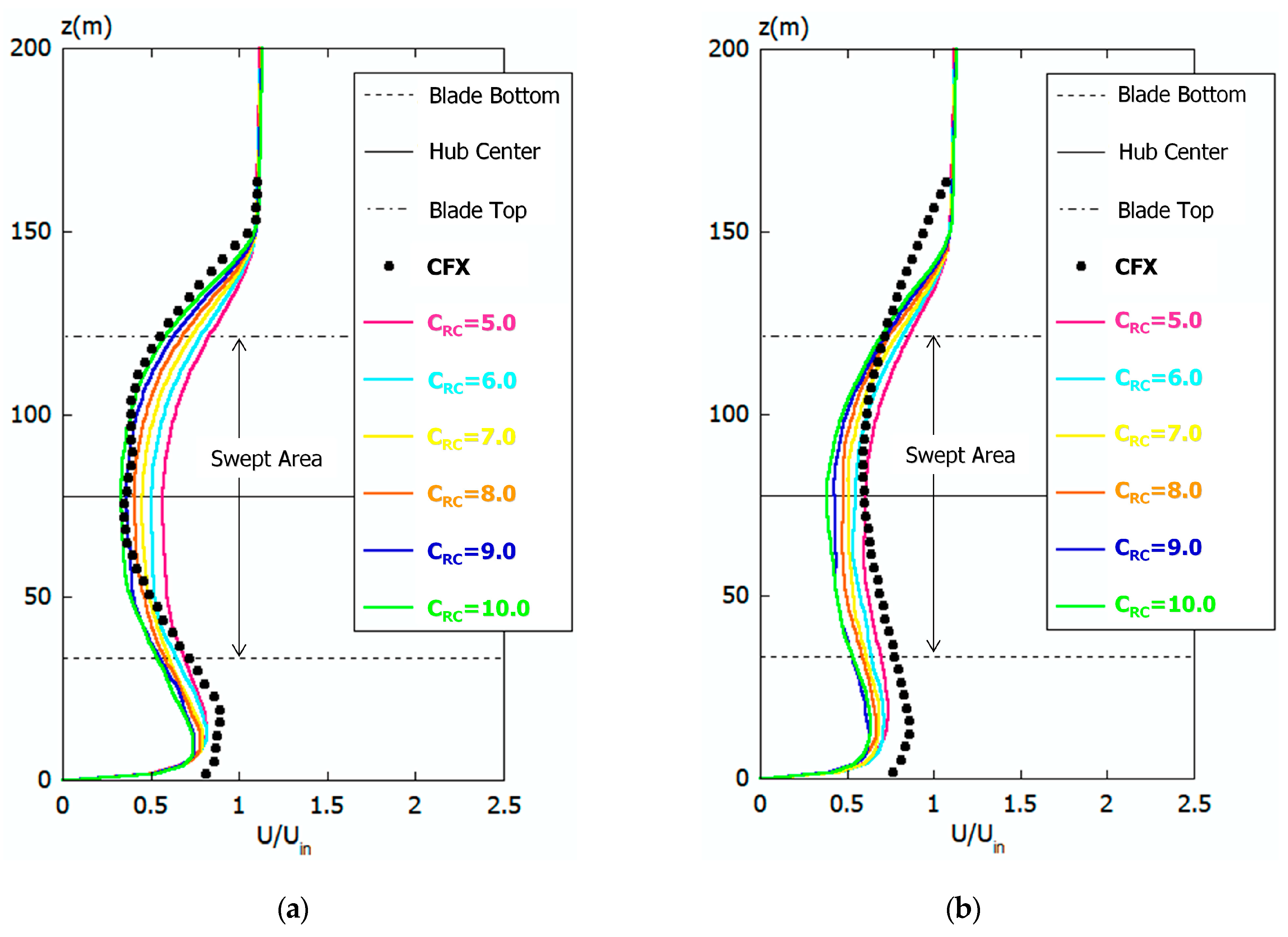
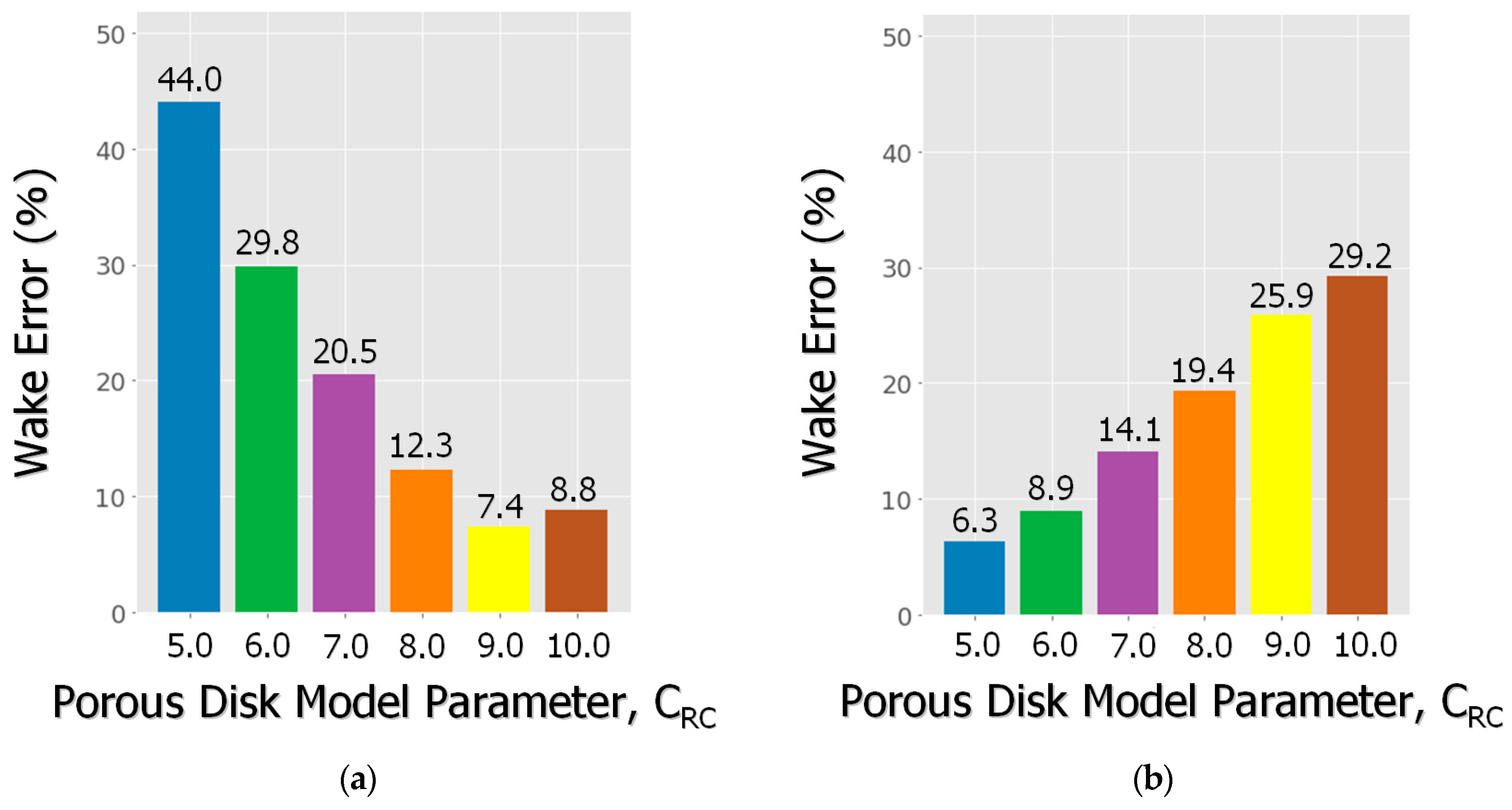
Figure 20 shows a comparison of the vertical distribution of time-averaged U-velocities at (a) x = 5D (near wake region) and (b) x = 10D (far wake region), regarding the simulation results of the time-averaged field for the real wind turbine. Figure 21 shows the wake error calculated using Equation (1) based on the numerical results shown in Figure 20. Examining these results, at x = 5D (near wake region) downstream of the wind turbine, the result of model parameter C_RC = 9.0 or 10.0 of the CFD PD wake model has the smallest error from the numerical result determined by ANSYS(R) CFX(R). At x = 5D in the near wake region, it is considered that the separated flows from the wind turbine nacelle and tower strongly influence the formation of the wake region behind the wind turbine. On the other hand, at x = 10D (far wake region) downstream of the wind turbine, the result of the model parameter C_RC = 5.0 of the CFD PD wake model has the smallest error from the numerical result determined by ANSYS(R) CFX(R). As mentioned above, these results confirm that wind energy/wind farm developers can accurately predict the time-averaged velocity deficit at the separation distance by selecting an appropriate value for the model parameter C_RC. In addition, further examination on the spatial distribution of model parameter C_RC set in the swept area of the wind turbine is required for a wide range of wind speed classes and different wind turbine sizes including large offshore wind turbines of 10 MW or higher power levels.

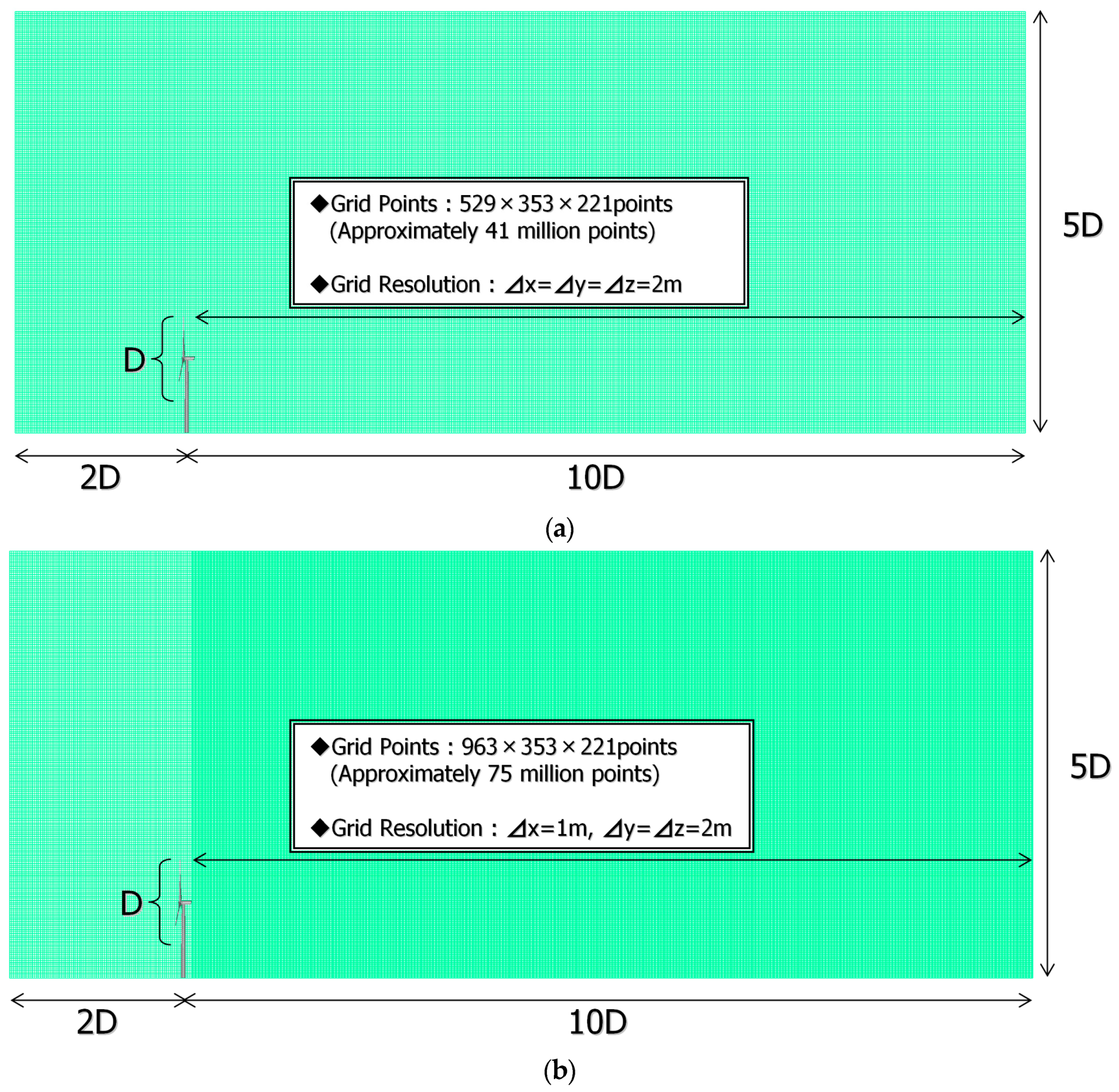
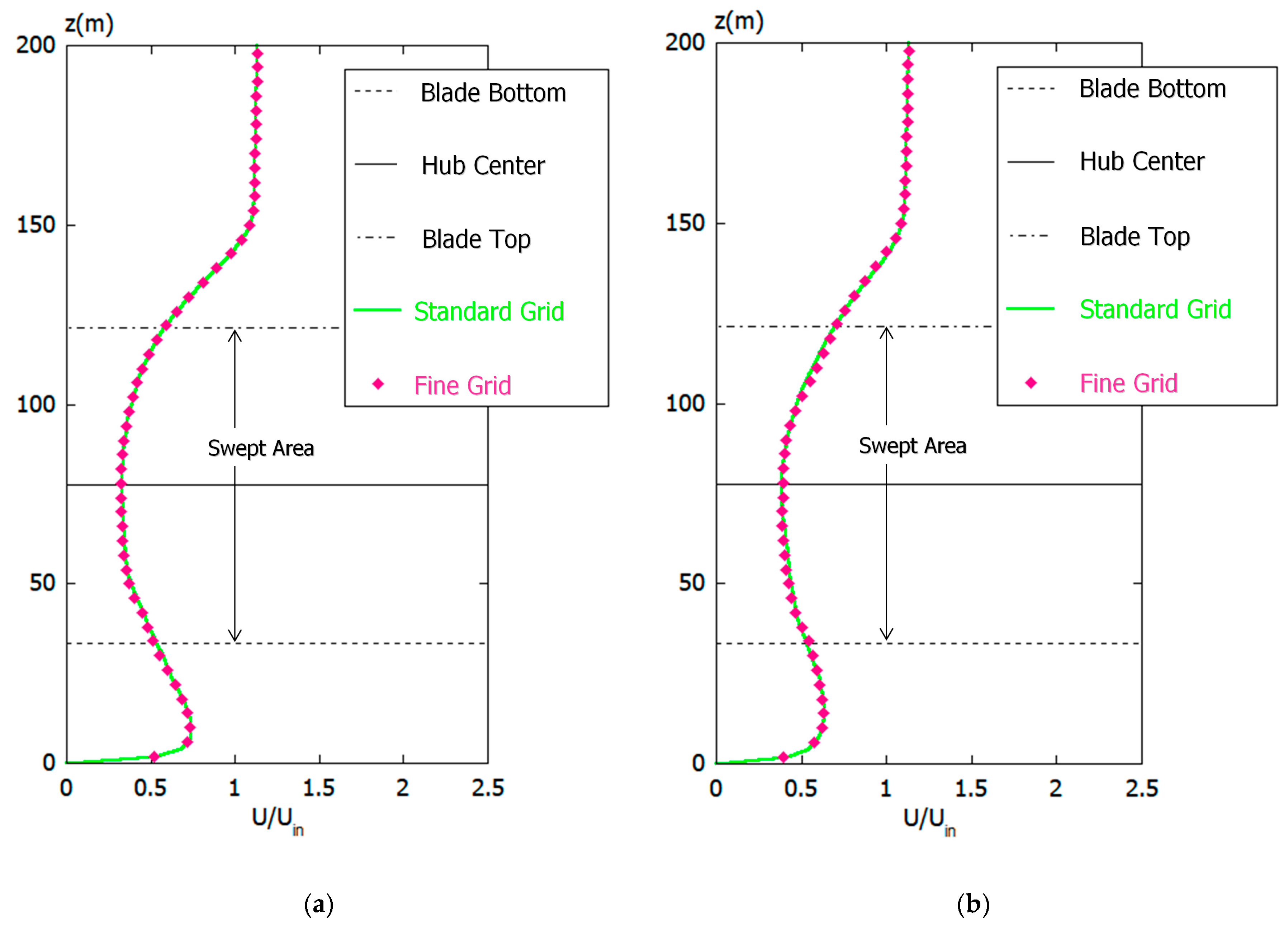
In the present study, we also examined the effect of spatial grid resolution when using the CFD PD wake model. Figure 22 shows a comparison of computational grids. The computational grid, called the standard grid, shown in Figure 22a, was used in the numerical results described so far. In contrast, in the fine grid shown in Figure 22b, only the spatial grid resolution in the streamwise direction (x) is doubled downstream of the wind turbine (Δx = 2 m → 1 m). Here, the spatial grid resolution in the spanwise direction (y) and vertical direction (z) is the same in both the standard grid shown in Figure 22a and the fine grid shown in Figure 22b.

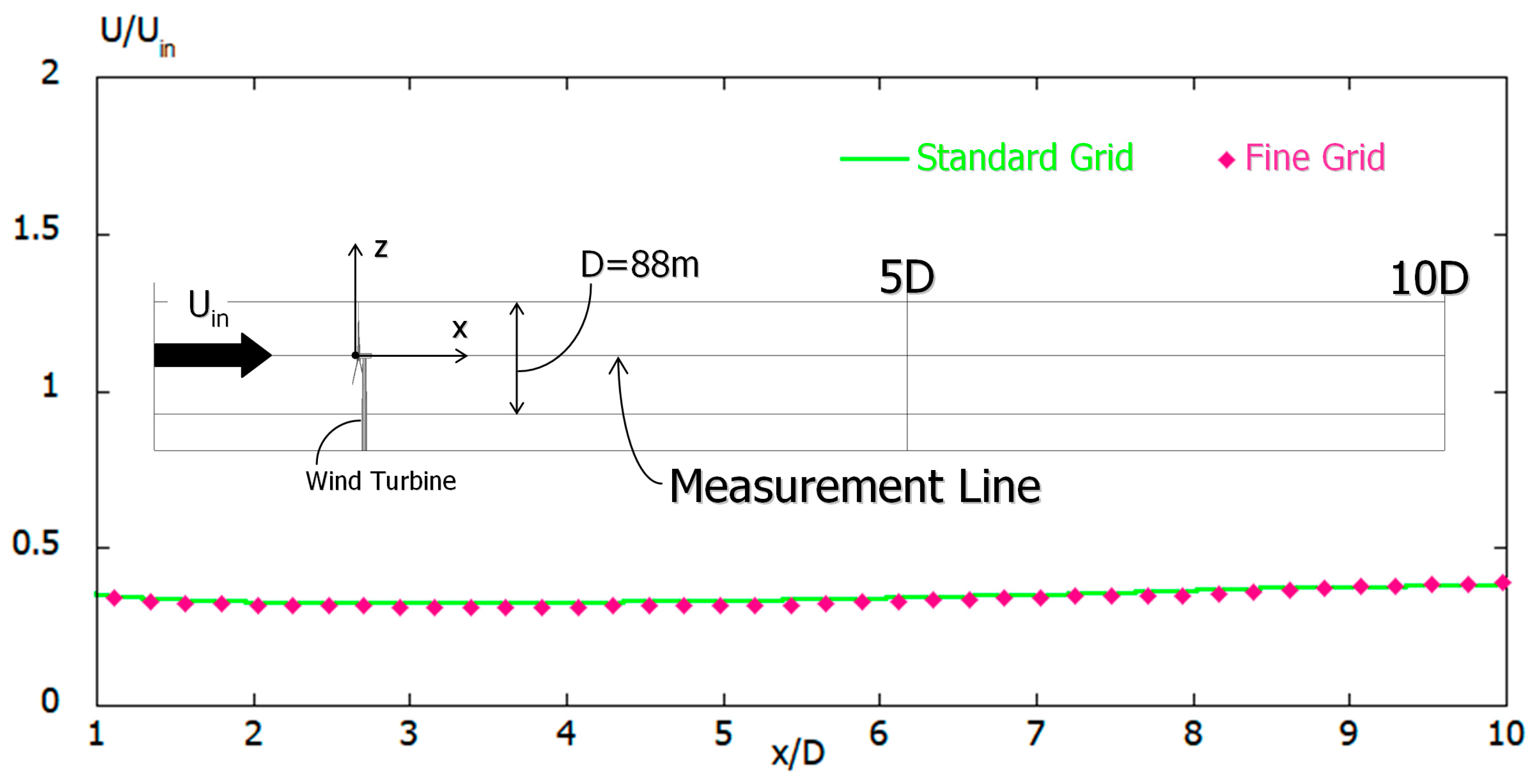
Figure 23 shows a comparison of the spatial distribution of time-averaged U-velocities at the hub center of the wind turbine with respect to the time-averaged flow field. Figure 24 shows the comparison of the vertical distribution of time-averaged U-velocities at (a) x = 5D (near wake region) and (b) x = 10D (far wake region) for the numerical results of the time-averaged field. Through comparison of these results, it was confirmed that there was no significant difference between the numerical results using the standard grid and the numerical results using the fine grid.

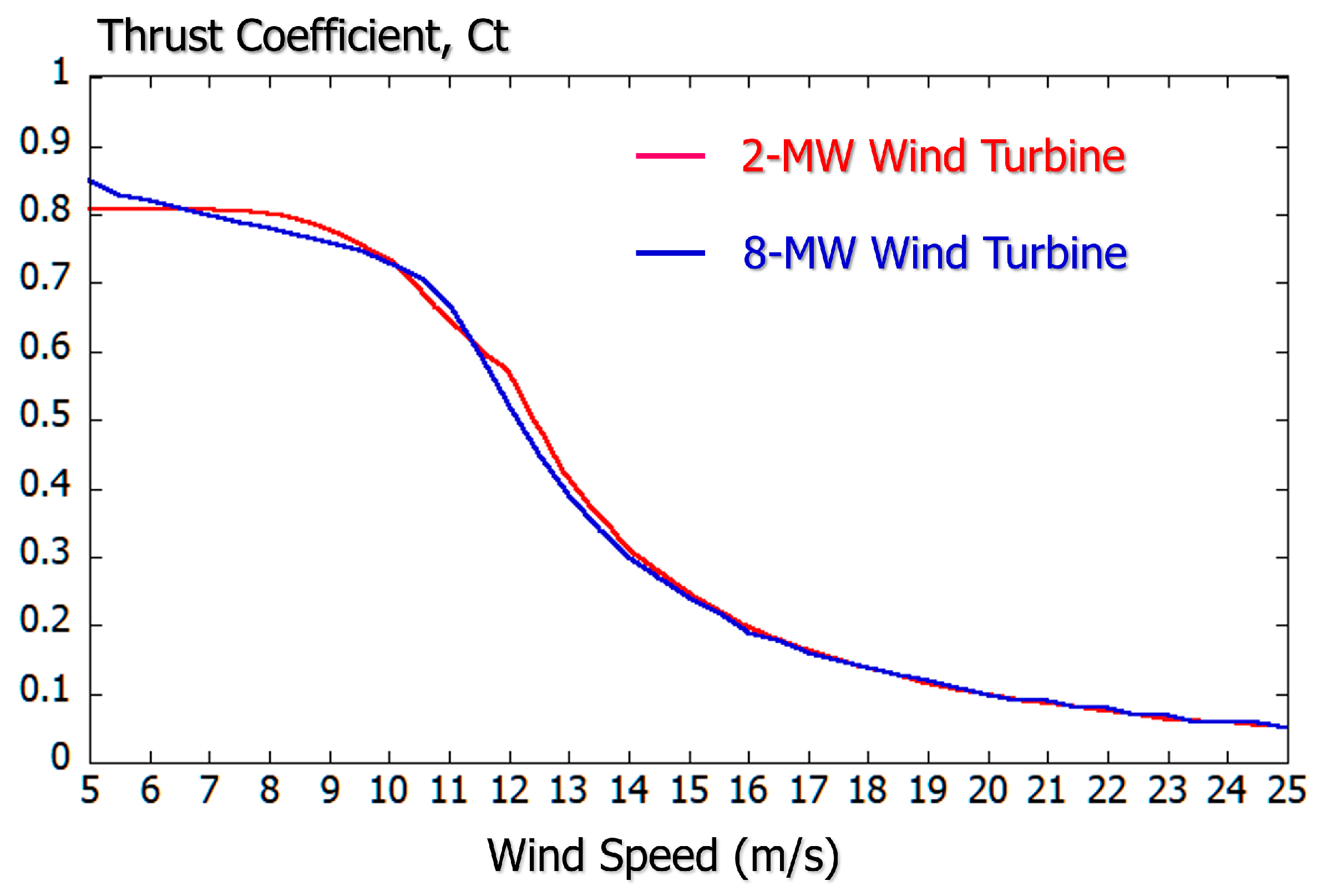
Finally, Figure 25 shows the relationship between the wind speed (horizontal axis) and the thrust coefficient Ct (vertical axis) for various real wind turbines for 2- and 8-MW wind turbines [28,29]. From this figure, it can be seen that the thrust coefficients Ct of both show almost the same value in all wind speed classes. This result suggests that it is appropriate to use the thrust coefficient Ct as the dominant parameter for wind turbine wake, regardless of the scale of the wind turbine and the control method of the wind turbine. In other words, it is highly expected that the new CFD PD wake model we proposed will be applicable to a wide range of wind speed classes and various wind turbine sizes by further improvement in the future.

5. Conclusions

In this study, the new CFD PD wake model was proposed in order to accurately predict the time-averaged wind speed deficits in the wind turbine wake region formed on the downstream side by the 2-MW wind turbine operating at a wind speed of 10 m/s. We use the concept of forest canopy model as a new CFD PD wake model, which has many research results in the meteorological field. In the forest canopy model, an aerodynamic resistance is added as an external force term to all governing equations (Navier–Stokes equations) in the streamwise, spanwise, and vertical directions. Therefore, like the forest model, the aerodynamic resistance is added to the governing equations in the three directions as an external force term in the PD wake model. In addition, we have positioned the newly proposed the LES using the CFD PD wake model approach as an intermediate method between the engineering wake model (empirical/analytical wake model) and the LES combined with AD or AL models. The newly proposed model is intended for use in large-scale offshore wind farms (WFs) consisting of multiple wind turbines (see Appendix B).

In order to verify the validity of the new CFD PD wake model proposed in the present study, we compare it with huge computation results using fully resolved geometries combined with unsteady RANS by use of the ANSYS(R) CFX(R) software. First, a 1/88 scale model (rotor diameter D = 1 m) of a 2-MW wind turbine (rotor diameter D = 88 m and wind turbine hub height of 75 m) was installed in a wind tunnel. The obtained simulation results were compared with the results of airflow measurement using a wind tunnel. In the numerical simulation by ANSYS(R) CFX(R), the effect of the difference in spatial grid resolution set on the wind turbine blade surface on the wind speed distribution in the wind turbine wake region was verified. As a result, within the range of the spatial grid resolution set in the present study, it was shown that the fully resolved geometries combined with unsteady RANS approach, using ANSYS(R) CFX(R), is able to appropriately reproduce the flow phenomena in a wind tunnel experiment using a scale wind turbine model.

Next, based on the knowledge of the spatial grid resolution of the wind turbine blade surface obtained from the simulation results for the wind tunnel experiment, a huge computation for a 2-MW real-scale wind turbine (rotor diameter D = 88 m and wind turbine hub height of 75 m) was performed. Based on the obtained simulation results, a time-averaged wind speed database in the wind turbine wake region was created. The optimal model parameter C_RC was estimated by comparing the time-averaged wind speed database in the wind turbine wake region by the previously described fully resolved geometries combined with unsteady RANS found by ANSYS(R) CFX(R). As a result, in the range from x = 5D of the near wake region to x = 10D of the far wake region, by selecting model parameter C_RC corresponding to the separation distance that wind energy/wind farm developers pay attention to, it was clarified that it is possible to accurately evaluate the time-averaged wind speed deficits at a given separation distance. For example, if wind energy/wind farm developers want to know the exact time-averaged velocity deficit at x = 5D, they should set C_RC to 9.0 or 10.0, or if they want to know the exact time-averaged velocity deficit at x = 10D, they should set C_RC to 5.0. We also examined the effect of the spatial grid resolution using the CFD PD wake model proposed in the present study and clarified that the spatial grid resolution has little effect on simulation results shown here.

In this research, only the wake flow of the 2-MW wind turbine with an 88-m-diameter rotor at a wind speed of 10 m/s was targeted, but we plan to apply the new CFD PD wake model to large-scale offshore wind farms (WFs) consisting of multiple wind turbines and quantitatively investigate the reproducibility of the interaction between wind turbine wakes, which are nonlinear flow phenomena in the near future. Furthermore, we will consider improvement to the PD wake model that can support a wide range of wind speed classes and various wind turbine sizes including large offshore wind turbines of 10 MW or higher power levels.