Article

Performance Analysis of a H-Darrieus Wind Turbine for a Series of 4-Digit NACA Airfoils

by
Krzysztof Rogowski
1,*,
Martin Otto Laver Hansen
2 and
Galih Bangga
3
1
Institute of Aeronautics and Applied Mechanics, Warsaw University of Technology, 00-665 Warsaw, Poland
2
Department of Wind Energy, Technical University of Denmark, DK2800 Lyngby, Denmark
3
Institute of Aerodynamics and Gas Dynamics, University of Stuttgart, 70569 Stuttgart, Germany
*
Author to whom correspondence should be addressed.
Energies 2020, 13(12), 3196; https://doi.org/10.3390/en13123196
Submission received: 24 April 2020 / Revised: 16 June 2020 / Accepted: 16 June 2020 / Published: 19 June 2020
(This article belongs to the Section A3: Wind, Wave and Tidal Energy)

Abstract

:
The purpose of this paper is to estimate the H-Darrieus wind turbine aerodynamic performance, aerodynamic blade loads, and velocity profiles downstream behind the rotor. The wind turbine model is based on the rotor designed by McDonnell Aircraft Company. The model proposed here consists of three fixed straight blades; in the future, this model is planned to be developed with controlled blades. The study was conducted using the unsteady Reynolds averaged Navier–Stokes (URANS) approach with the k-ω shear stress transport (SST) turbulence model. The numerical two-dimensional model was verified using two other independent aerodynamic approaches: a vortex model and the extended version of the computational fluid dynamics (CFD) code FLOWer. All utilized numerical codes gave similar result of the instantaneous aerodynamic blade loads. In addition, steady-state calculations for the applied airfoils were also made using the same numerical model as for the vertical axis wind turbine (VAWT) to obtain lift and drag coefficients. The obtained values of lift and drag force coefficients, for a Reynolds number of 2.9 million, agree with the predictions of the experiment and XFOIL over a wide range of angle of attack. A maximum rotor power coefficient of 0.5 is obtained, which makes this impeller attractive from the point of view of further research. Research has shown that, if this rotor were to work with fixed blades, it is recommended to use the NACA 1418 airfoil instead of the original NACA 0018.

1. Introduction

In 1931, G. J. M. Darrieus, a French aviation engineer, patented a wind turbine rotor capable of operating independently of the wind direction and in adverse weather conditions. The Darrieus wind turbine, having a rotor with a vertical rotation axis, is often used to convert wind energy into electric energy. The Darrieus wind turbine is composed of several curved blades attached to a vertical rotating shaft. In 1927, G. Darrieus also suggested other possible solutions for turbines with a vertical rotation axis. One of them was H-rotor (rotor in H pattern), also known as “H-bar”. The rotor of this type consists of long straight blades, which are usually fastened to the tower by means of horizontal struts. Giromill is another type of wind turbine with articulated and controlled straight blades to ensure maximization of energy extraction from the wind flow [1], and the McDonnell 40 kW giromill is an example of such a construction (Figure 1). This wind turbine was designed and built in the mid-1970s by McDonnell Aircraft, which won a contract from the forerunner of the U.S. Department of Energy. Available literature on the McDonnell wind turbine provides information on the basic geometrical and construction parameters of this rotor, as well as on its operating parameters [2,3,4]. Aerodynamic characteristics of the giromill were investigated in a wind tunnel and in the field; however, they are optimistic enough to examine this configuration again. Jankowski [5] conducted research on this construction using the single-streamtube model (SSM). He proved that both a clean rotor (rotor with infinite aspect ratio and without struts and rotating shaft) with controlled blades, as well as a rotor with zero pith, can achieve a maximum power coefficient of approximately 0.5. The literature review made by the authors does not show any advanced numerical research of this wind turbine. At that time, Anderson et al. [1], employing the Larsen Cyclogiro Performance Computer Program, estimated the device’s maximum power factor of 0.51. This is quite a high value, even when compared to the performance of modern horizontal-axis wind turbines (HAWTs) [6]. The results of the power curve obtained from the measurements of this rotor are also promising [3]. The current work uses the geometry of the McDonnell Aircraft Company 40 kW design as a baseline for further research. The purpose of this work is to confirm the actual efficiency of this rotor, while first considering a rotor with fixed blades. Basic geometrical data of this rotor are given in Table 1.
The reason mentioned in the paragraph above is not the only reason for this topic. In recent years, many experimental and numerical studies of micro scale vertical-axis wind turbines have been carried out [7,8,9,10,11,12,13,14,15,16,17,18,19]. A lot of research is also underway in the field of multi-megawatt offshore Darrieus-type wind turbines [20,21,22]. The number of investigations of medium power rotors is quite limited in this context [23,24]. However, as the market demand shows, there is a great demand for this type of construction [25]. This is due to their advantages, such as, for example, lower manufacturing cost, omni-directional capability, and lower noise [14]. This argument also prompts further research on medium power wind turbines.
For rotors with a vertical axis of rotation, choosing the right airfoil is a key issue but also extremely difficult. This is related to the transient operation characteristics of this rotor type, which results from the constant change of the blade’s angle of attack and the pulsation of aerodynamic blade loads during each rotor revolution. In addition, the Darrieus wind turbine rotor operates in a wide range of tip speed ratios. All this means that the rotor can experience adverse effects of dynamic stall, as well as blade-wake interactions [26,27]. The nature of the work of this type of rotor is also affected by, among others, the rotor size, solidity, and Reynolds number [1]. All of this only increases the difficulty in selecting the appropriate airfoil. The selection of the aerodynamic airfoil is most often made using numerical methods of fluid dynamics, less often by use of experimental tests [15,28,29,30,31,32,33,34]. Most of these studies mainly considered wind turbines operating in the range of small Reynolds numbers. Bedon et al. [32] studied large scale wind turbines operating at a tip speed ratio range between 1 and 9 and at Reynolds number range between 100,000 and 3,000,000. Their work, however, focused on symmetrical airfoils: NACA 0015, NACA 0018, NACA 0021, and NACA 0025.
Four-digit NACA airfoils developed by National Advisory Committee for Aeronautics (NACA) describe the contour shape of an aircraft wing or a cross section of a wind turbine blade. The shape of the airfoil is described by means of a mathematical formula, given, among others, by Moran [35]. The shape of the 4-digit NACA airfoil series really depends on three parameters: the maximum airfoil thickness, t, as a fraction of the chord (this value is expressed in the 4-digit airfoil denomination using the last two digits divided by 100); the maximum camber, m, (100∙m gives the first digit of the 4-digit airfoil denomination); and the location of the maximum camber, p, (10∙p gives the second digit in the NACA XXXX airfoil denomination). For symmetrical airfoils, only the maximum thickness is needed for the complete airfoil description; the other two parameters, the maximum camber and the location of the maximum camber, are used to design asymmetrical profiles.
Four-digit NACA symmetrical airfoils are probably the most commonly used foils in the design and manufacture of Φ-type and H-type Darrieus wind turbines. Vertical-Axis Wind Turbines (VAWT) Ltd., a company from Great Britain, also proposed a H-type rotor with straight blades called a Musgrove rotor [36]. The largest prototypes produced by this company were the VAWT-450 (rated power of 130 kW) and VAWT-850 (rated power of 500 kW); the first of them had the NACA 0015 airfoil, and the second one had the NACA 0018 airfoil [37,38,39]. Other, more modern, experimental studies of H-type rotors were conducted, among others, at Uppsala University. The 200 kW VAWT prototype with three straight blades was installed in early 2010 in Falkenberg, Sweden. This rotor, having NACA 0018 airfoils, provided 22.5 MWh of energy to the power grid during the tests within 1000 h of operation [40,41]. In the case of Φ-type rotors, in most commercial cases, symmetrical airfoils of the 4-digit NACA series were used [1,25,37,42].
Many authors have studied the aerodynamic performance of VAWTs equipped with one specific airfoil type, usually the NACA 00XX. Rezaeiha et al. [17] studied a 1-bladed vertical-axis wind turbine with the NACA 0015 airfoil using the scale adaptive simulation (SAS), unsteady Reynolds averaged Navier–Stokes (URANS), and hybrid Reynolds averaged Navier–Stokes (RANS)/large eddy simulation (LES) methods. Their main purpose was to investigate the properties of dynamic flow detachment on the rotor blade at a low tip speed ratio. Another valuable numerical work of these authors was devoted to the research of three different small sizes wind turbines [18]. Zong et al. [43] proposed a method of passive control of dynamic stall of Darreius wind turbine blades. The authors proposed to install a small rod in front of the leading edge of the symmetrical NACA 0018 airfoil. Wong et al. [44] performed a 3-D numerical analysis of a rotor having straight blades with NACA 0021 airfoils. They studied the effects of a flat plate deflector placed upwind of the vertical wind turbine. Elsakka et al. [45] found a method to calculate and store the local angle of attack for VAWT over the entire cycle from CFD. These authors examined the distribution of the local angle of attack of the NACA 0015 airfoil blade. This could be also estimated by performing system identification, which is often used in aerodynamic modeling for time [46] or frequency domain [47]. Experimental and numerical testing of the three-bladed rotor was performed by Bianchini et al. [48]. These authors confirmed the usefulness of the Shear Stress Transport (SST) turbulence model to study the aerodynamic characteristics of the H-Darrieus rotor with blades having the NACA 0021 airfoils. Bianchini et al. [49] and Bianchini et al. [50] studied the behavior of the symmetrical NACA 0018 airfoil in “Darrieus motion” and noticed that the results of the aerodynamic blade loads correspond to the cambered airfoil, a phenomenon called “virtual camber effect” that comes from the fact that they operate in a curved inflow. Airfoil shape effect of a three-bladed rotor with a solidity of 0.1 was investigated by Mohamed et al. [51] using many symmetrical and asymmetrical airfoil types. The symmetrical NACA 0015 airfoil showed equally high aerodynamic efficiency as the best among the tested airfoils. NACA 4-digit airfoils also provide good aerodynamic characteristics of Darrieus-type rotors working in water [52]. Sometimes a classic 4-digit NACA airfoil is the starting point in the airfoil shape optimization process [53].
A literature review shows that many scientific works have been devoted to the issue of the impact of airfoil shapes on the Darrieus wind turbine performance. However, most of the cited works relate to small scale rotors, as well as wind turbines, in MW scale. Therefore, there is a need to extend the research for medium power Darrieus wind turbines. Moreover, various airfoil shape optimization works mainly deal with aerodynamic blade loads and their impact on rotor power coefficient. In this work, the influence of profile shape on rotor performance but also on the shape of velocity profiles downstream behind the rotor was examined. This gives an additional criterion in the optimization process.
The current work focuses on comparing the aerodynamic performance of a three-bladed H-Darrieus with 4-digit NACA airfoils depending on two parameters: the maximum airfoil thickness and the maximum camber. The shapes of the analyzed airfoils are shown in Figure 2.

2. Rotor Aerodynamic Performance

The operating rotor of the vertical-axis wind turbine creates aerodynamic loads that causes a local slowdown of the main flow. The forces change with the azimuth, θ, which defines the location of the rotor relative to the wind direction. In this work, azimuth zero means the position of the rotor in which the chord of the rotor blade is parallel to the main flow direction and the blade moves “against the wind”. In the present work, azimuth is measured from zero value, as shown in Figure 3. When the azimuth changes, the local angle of attack, as well as local blade loads, also change. The loads also depend on other factors, such as, for example: the rotor solidity, the blade Reynolds number, airfoil shape, and the tip speed ratio. The aerodynamic loads of blades are most often represented as coefficients, defined as follows:
C F N ,   T = F N ,   T 1 2 ρ V 0 2 A ,
where FN, T are the aerodynamic blade load components, normal and tangential, respectively; V0 is the wind velocity; ρ is the air density; A is the reference surface; in this work, A = c∙1, where c is the length of the chord, and 1 is the unit span of the blade. The tip speed ratio is defined as the ratio of tangential blade velocity VT and wind velocity:
T S R = V T , V 0 = ω R V 0 ,
where ω is the angular velocity of the rotor, and R is the rotor radius.
In this work, the authors not only analyzed the distribution of aerodynamic blade loads but also the distributions of flow velocity in the aerodynamic wake behind the rotor. The velocity distribution is a direct result of the aerodynamic blade loads. In this work, two components of the velocity downstream behind the rotor were analyzed: a component parallel to the wind direction, Vx, and a perpendicular component, Vy. These velocities were calculated using a rake that consists of 100 checkpoints, positioned at a distance of 1.5 R downstream behind the rotor axis of rotation, as shown in Figure 4. The total length of the rake was 3∙R, similar to the case of the experiments of Tescione et al. [54,55]. The velocity components Vx and Vy vary in time, but this paper presents their average values according to the formula:
V x ,   y = 1 T 0 T V x ,   y ( t ) d t ,
where the averaging time, T, corresponds to the time of one full rotation of the rotor and the time integration step, which is equal to time step size.

3. Numerical Model

All the numerical results of the Darrieus wind turbine aerodynamic characteristics presented in this article were obtained using the CFD tool, ANSYS Fluent, Release 17.1. This section describes the geometric model, grid distribution and solver settings.

3.1. Geometric Modeling

The calculations were carried out for the 40 kW Giromill rotor presented in Section 1 and in Figure 1. The real rotor has many elements that are not included in our numerical model. The current considerations did not take into account such structural elements as: blade supports, as well as the rotating and fixed towers. The original rotor had controlled blades, but, in this work, only the rotor with fixed blades was investigated. In addition, the rotor was tested using a two-dimensional model consisting of three aerodynamic airfoils rotating around a fixed axis, as depicted in Figure 3. Rotor blades represented by two-dimensional NACA airfoils are treated as rigid bodies.
This rotor model was placed in a virtual wind tunnel (computational domain) that is large enough to eliminate the tunnel blockage effects; thus, no tunnel correction model is needed. The rectangular computational domain with dimensions of 20 R by 60 R is presented in Figure 4. Choosing computational domain sizes is one of the critical issues of modeling [27], but, based on following papers, the domain size should be sufficiently large. Beri and Yao [56] showed that a ratio of domain width to rotor diameter of 6 is enough to correctly estimate the rotor power coefficient. Mohamad et al. [57] studied the effect of computational domain size for a Savonius rotor performance, and they showed that the ratio of the computational domain width to the Savonius rotor diameter of 10 gives sufficiently accurate rotor torque results. Rogowski [13] received a similar conclusion when examining the influence of the square-length computational domain for a Darrieus rotor. Therefore, in our considerations presented in this paper, the ratio of domain width to rotor diameter was chosen to be 10. The distance from the rotor axis to the inlet was assumed to be 5 D [27]. The distance between the rotor axis of rotation and the outlet is equal to 25 D, slightly larger than in the case of Ferreira et al. [58] and smaller than in the case of Castelli et al. [59] or Trivellato and Castelli [60].
Transient flow around the rotating rotor was considered in this work. This issue requires the use of a special technique of moving meshes. The use of this technique, also known as the “sliding mesh” approach, requires the separation of a certain domain area surrounding the rotating rotor. The distance between the common edge of both areas and the edge of the airfoils should be large enough due to possible numerical errors [9]. In our case, this area has the shape of a circle with a diameter of 2D, as shown in Figure 4.

3.2. Numerical Settings

In these investigations, transient analyzes of the operating VAWT were performed; therefore, the Unsteady Reynolds Averaged Navier–Stokes (URANS) approach was utilized. The following instantaneous governing conservation equations of continuity and momentum are solved during the simulation can be written form as (ANSYS, Inc., release 17.1):
u i x i = 0 ,
u i t + ( u i u j ) x j = 1 ρ p x i + x j ( 2 ν S i j u i u j ¯ ) ,
where u i and u j are velocity components; ν is the kinematic viscosity; S i j is the strain-rate tensor defined as: S i j = 1 / 2 ( u i / x j + u j / x i ) . The last term in Equation (5) is the Reynolds-stress tensor, which, for constant density, is defined as: τ i j = u i u j ¯ .
Algorithms used in this work to solve governing equations were presented in previous work [61,62]. Transient calculations were performed using the sliding mesh technique available in ANSYS Fluent, Release 17.1 CFD code. This involves using an inner circular zone that rotates at the same angular velocity as the wind turbine rotor relative to the rectangular fixed outer zone. In this model, mesh nodes of the dynamic zone move rigidly. In addition, the rotating and stationary zones are connected with each other using a non-conformal interface. During the simulation of transient flow around an operating rotor the transport equations of momentum, continuity and turbulence are solved for defined time step. This time step size Δt is most often taken constant and corresponds to a certain increase in azimuth Δθ = ω∙Δt. The choice of time step size length is a particularly important issue in the numerical calculations of Darrieus rotor. According to the ANSYS Documentation (ANSYS, Inc., release 17.1), the length of the time step size should be small enough for the required level of convergence of the solving equations to be obtained in the defined maximum number of iterations per time step. In addition, Rogowski [19] showed that, even if the assumed time step satisfies the desired convergence criterion, it may not be sufficient to capture all aerodynamic phenomena, such as, for example, the effect of the tower’s aerodynamic shadow on wind turbine blade loads. Rogowski [19] and Rezaeiha et al. [17] agree that, for a “clean rotor” (a rotor consisting only of blades), the length of the time step can be assumed equivalent to an azimuth increase, Δθ, of 0.1 degrees, with the maximum iterations of 20 per time step; therefore, exactly such time step settings were adopted in these simulations.
Turbulence modeling is another key issue in the CFD approach. In practice, it requires the determination of the last term in Equation (5)—the Reynolds-stress tensor τ i j . In various CFD codes, this is done using so-called turbulence models. In the URANS approach, two-equation turbulence models of the k-ω and k-ε families are most commonly used, while the one-equation Spalart-Allmaras turbulence model of Balduzzi et al. [27] is less often used. This work is not dedicated to investigating the impact of the turbulence model on solving the problem of transient flow around a working rotor. Current simulations use a model widely used in this kind of flows [19], the Shear-Stress Transport (SST) k-ω model. This two-equation turbulence model developed by Menter [63] is based on both the k-ε model proposed by Wilcox and the k-ε model that was proposed by Launder and Spalding. The k-ω SST turbulence model is actually a hybrid model that combines the k-ω formulation in the inner region of the boundary layer and the k-ε model in the bulk flow. Thanks to advantages of this model and larger accuracy compared to the standard k-ε and k-ω models, it is commonly used in a wide flow class, especially in adverse pressure gradient flows or airfoils.

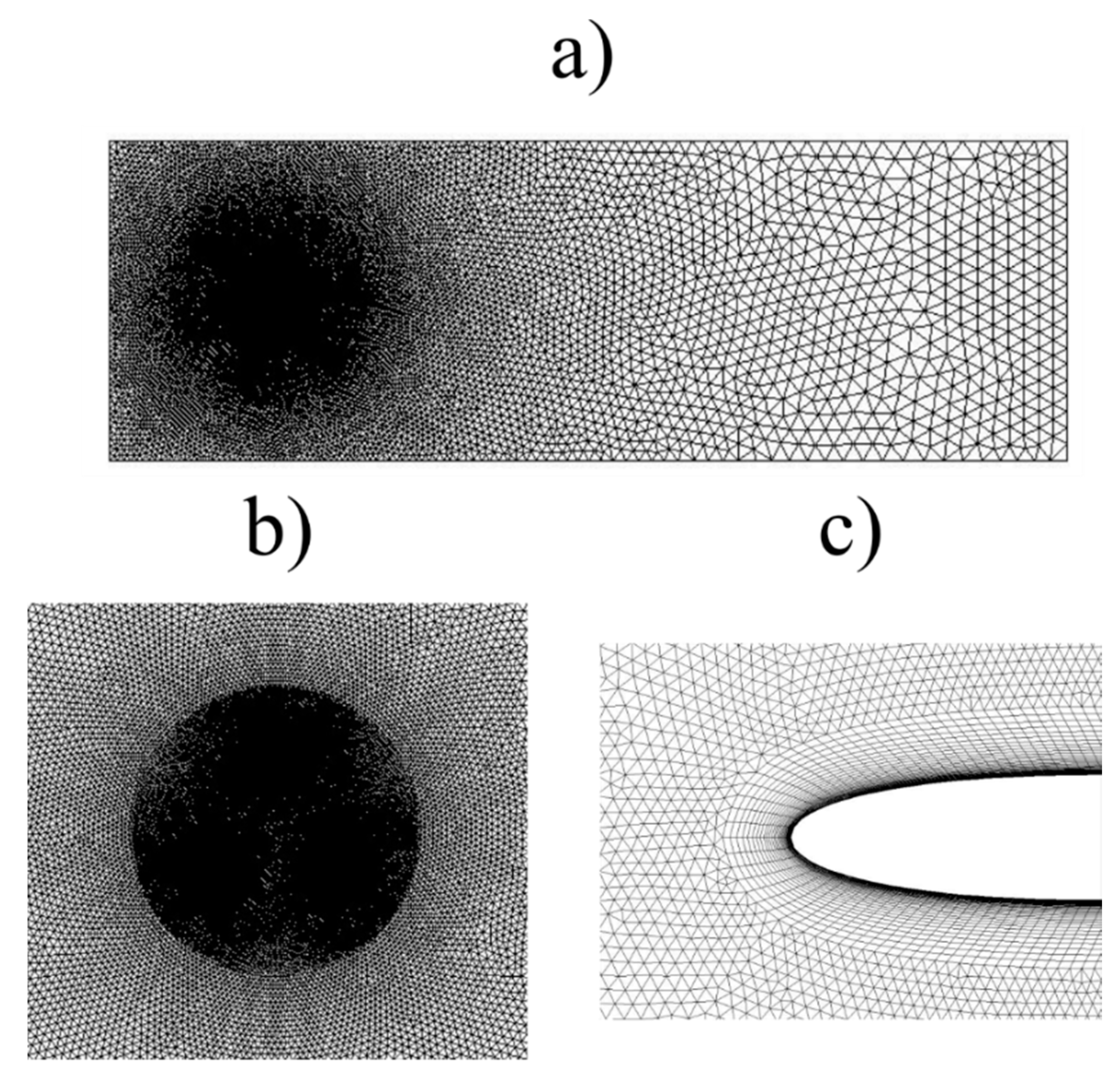
3.3. Computational Mesh

The computational grid is a hybrid mesh composed of a structural mesh near the airfoil edges to resolve the viscous boundary layer and an unstructured mesh in the remaining area. Near the edges of the airfoils, rectangular elements were used, and in the case of unstructured mesh, triangular elements. All numerical models investigated in this work, have the same global grid settings. The edges of the blades were divided into 200 elements of equal length. In the direction normal to the airfoil, the structural mesh has 60 layers, with the growth rate of 1.12, and the thickness of the first layer near the airfoil edges of 5.3 × 10⁶ m, which provides an average wall y+ of 0.50 for TSR = 2 and of 0.53 for TSR = 6. The growth rate of unstructured mesh elements is 1.04. The final grid shown in Figure 5 consists of 234,840 elements and 136,059 nodes. The computational grid with global settings described above was used also by Rogowski [19]. This author showed that these mesh settings provided sufficiently accurate results of the velocity fields and aerodynamic blade loads.

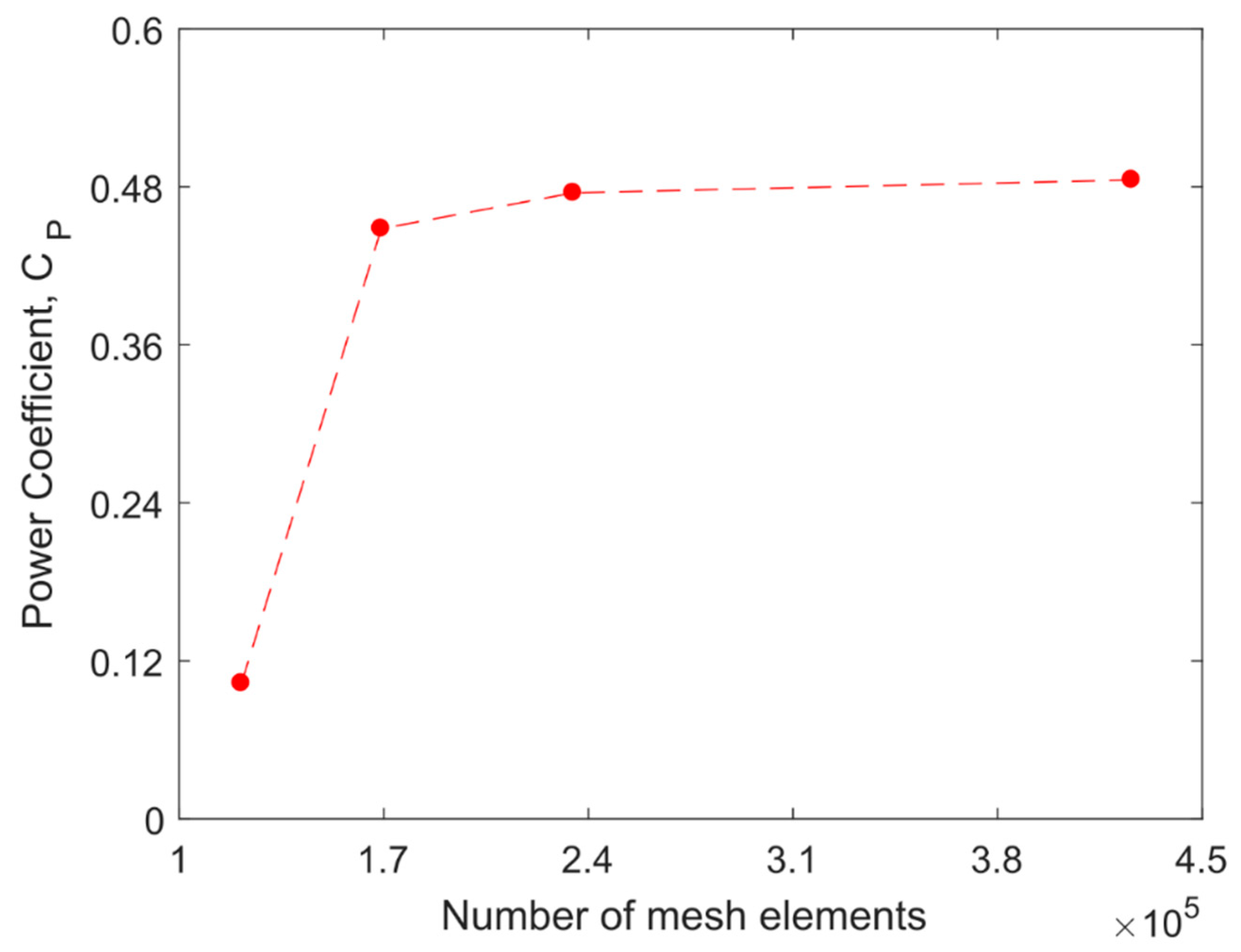
3.4. Mesh Sensitivity Study

The discrete model described in Section 3.3 has been tested to determine the number of elements that is required for accurate estimation of aerodynamic parameters. For this purpose, a series of additional simulations were carried out, in which the number of equal airfoil edge divisions was changed. According to Section 3.3, for all cases in this work, the number of equal airfoil edge divisions was N = 200, but calculations were also carried out for three cases: N / 4, N / 2, and 2∙N. A linear increase in the number of airfoil edge divisions also gives a linear increase in the total number of mesh elements from 121,350 for N / 4 to 425,892 for 2∙N. However, the biggest difference in power coefficient, CP, is for N / 4, i.e., for a number of divisions equal to 50. An increase in the number of elements above 200 does not cause a significant change in CP but leads to an increase in computational costs, Figure 6.

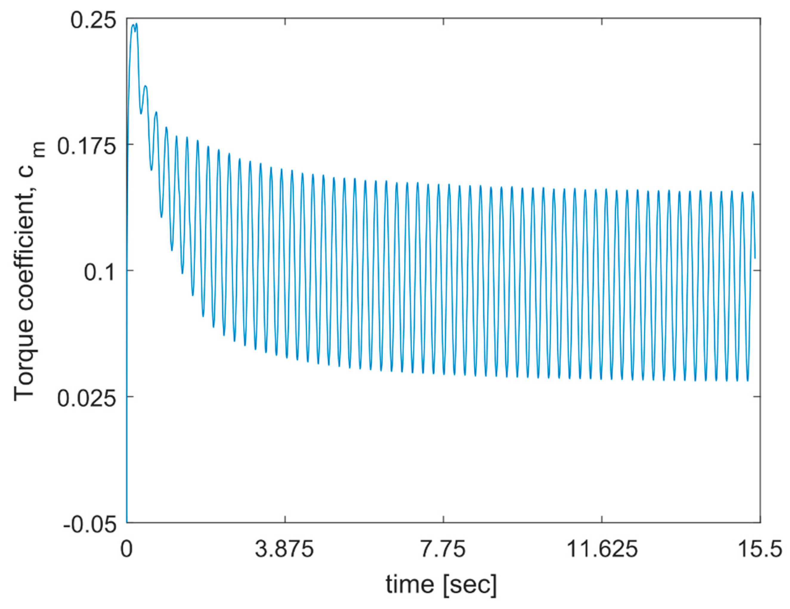
3.5. Initial Condition Effects

Before running numerical calculations, the initial conditions must be specified. Typically, homogeneous initial conditions are assumed throughout the entire domain; in this work, the initial conditions corresponded to the flow parameters at the inlet. During the simulation, transport equations are solved for each finite volume, and the correct flow parameters are determined. For each case studied, it is necessary to simulate several rotor revolutions to obtain a periodic result of the aerodynamic blade loads and velocity distributions in each subsequent rotor rotation. This transient is the physical time it takes the flow to become in equilibrium with the thrust force, i.e., the time to build up the induced wind speed.
Figure 7 shows the relation between the rotor torque coefficient, cm, and time. The rotor torque coefficient is defined as:
c m = T o r q u e 1 2 ρ A s R V 0 2 ,
where AS is the projected area seen by the wind, defined as = 2R∙1, where 1 is a unit span of the blade. The maximum values of the torque coefficient reach an almost constant values in each rotor revolution of about 1.3 after approximately 12 complete rotor revolutions. After 19 full turns, the differences are at the level of the second decimal place. The minimum values of this torque coefficient are about 0.03 after 12 full rotations of the rotor. A similar conclusion was made by Rogowski [19], who studied the effect of initial conditions by simulating 50 full rotor revolutions. Here, the simulation showed that 15 full revolutions of the rotor was sufficient to obtain repeatable results of both aerodynamic blade loads and velocity profiles behind the rotor.

4. Model Validation

Validation of the numerical model described in previous sections was performed in two ways. First, the lift and drag airfoil characteristics from the experiment of Sheldahl and Klimas [64] were taken into account as a baseline for steady-state CFD simulations. Then, the instantaneous normal and tangential aerodynamic blade loads computed using ANSYS Fluent, Release 17.1 CFD code were compared with the results obtained by the vortex model and FLOWer CFD code.

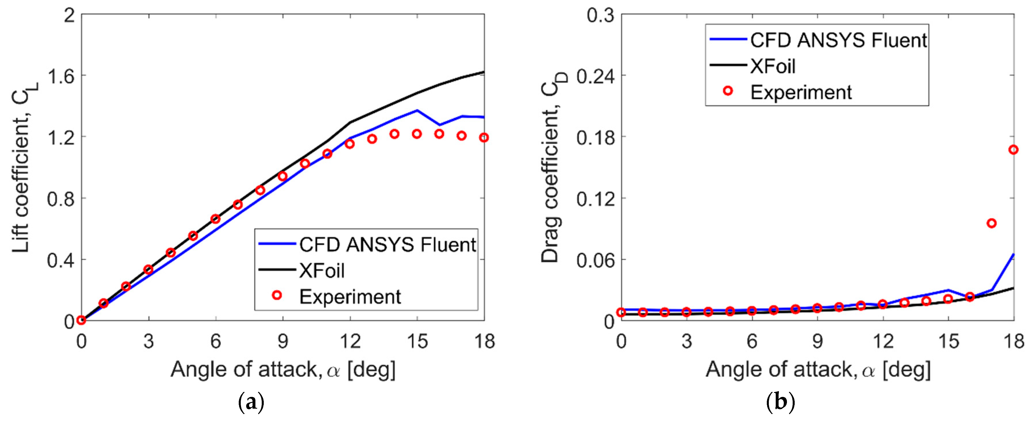
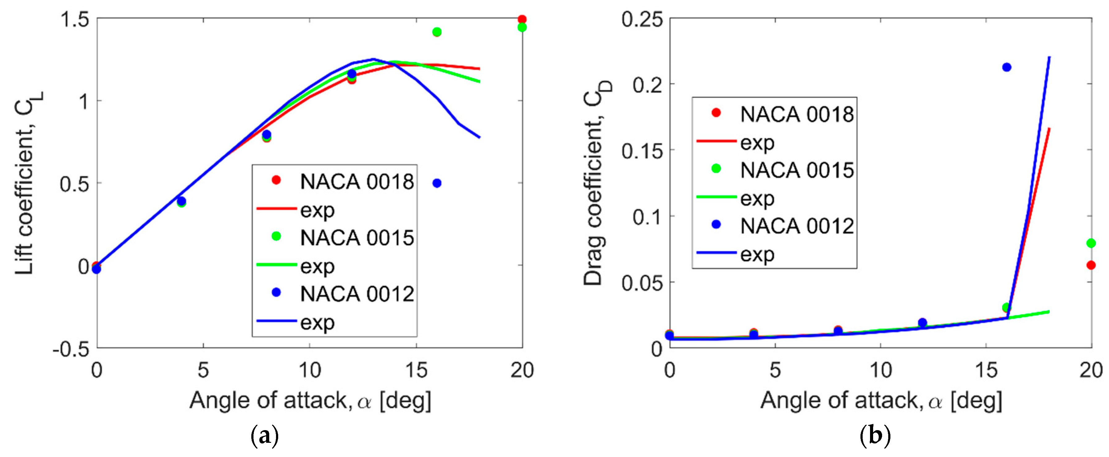
4.1. RANS Approach Validation Based on Measured Static Data for NACA 0018

Numerical calculations of aerodynamic force coefficients, lift and drag, for one rotor blade airfoil were carried out using the same computational mesh (Figure 5) as in the case of transient calculations of the entire rotor; the same turbulence model was also used as in the case of transient analysis. Mathematical formulation of governing equations for steady-state analysis is given by Equations (4) and (5); however, the term u i / t is equal to zero because the averaging time interval of the mean velocity tends to infinity. During steady-state numerical simulations, both parts of the computational mesh shown in Figure 5 remained stationary with respect to each other; the angle of attack of the analyzed airfoil remained unchanged during the simulation.
XFOIL code is very fast engineering tool for analysis of subsonic isolated airfoils. It is based on an inviscid linear-vorticity panel method taking into consideration a Karman-Tsien compressibility correction. The potential flow around the airfoil is modeled by applying source distributions on the airfoil and in the wake. The influence of viscous layers is taken into account by using a two-equation lagged dissipation integral method and the e9 method to find the location of the transition point. Inviscid formulation, governing equations for viscous formulation, and compressibility correction implemented in the interactive XFOIL are presented, among others, by Mark Drela [65].
A numerical experiment was carried out for the blade Reynolds number, defined as [1]:
R e = R ω c ν ,
where R is a rotor radius, ω is an angular velocity of the rotor; c is a chord length; and ν is kinematic viscosity of the air. This Reynolds number was used to determine the undisturbed flow velocity V0 for steady-state simulations. The undisturbed flow velocity in RANS simulations is equal to the tangential velocity of the rotating rotor blade, V0 = ωR. In these investigations, it was assumed that the angular velocity of the rotor was constant for all tip speed ratios and equal to 8.18 rad/s. Knowing that the rotor radius is 8.48 m, the tangential velocity of the rotor blade is 69.4 m/s for the Reynolds number to be equal to 2.9 million. Aerodynamic force coefficients, lift coefficient CL, and drag coefficient CD are defined as:
C L , D = L ,   D 1 2 ρ V 0 2 A ,
where L and D are lift and drag forces, ρ is air density, and A is reference area (in this investigation, A = c∙1, where 1 is unit span of an infinitely long rotor blade). Numerical results of these coefficients of aerodynamic forces were compared with experimental studies of Sheldahl and Klimas [64] and with the results obtained from the XFOIL program; these results are shown in Figure 8.
Discussing the presented results, it can be stated that both lift force coefficients, as well as drag coefficients obtained from CFD, are consistent with the experiment in the range of angles of attack from 0 to 14 degrees in the case of lift force and from 0 to 16 degrees in the case of drag force. From the zero lift, the CL curve is practically a straight line up to the angle of attack of 12–13 degrees. The aerodynamic derivative (dCL/dα) of the experimental CL curve for the angle range of 0–12 degrees is 5.681 per rad. The aerodynamic derivative of the CL curve from CFD is larger by 3.4% compared to the experiment, whereas the aerodynamic derivative from XFOIL is larger by 11% compared to the experiment. The minimum drag coefficient corresponds to the zero angle of attack and is 0.0076 for the experiment, 0.0061 for XFOIL, and 0.01 for CFD. The somewhat larger minimum drag for the CFD is most likely because transition was not considered.
As shown in Figure 8, the obtained CFD results are consistent with the prediction of the XFOIL program in the range of angles of attack up to about 14–15 degrees; then, the results given by XFOIL code are higher compared to CFD. These differences result from the modeling method in both used approaches; XFOIL code is based on the inviscid linear-vorticity panel method [65], whereas ANSYS Fluent, Release 17.1 CFD code solves Reynolds averaged Navier–Stokes (RANS) equations (Equations (4) and (5)). The accuracy of a CFD solution depends on many factors. One of them is the distribution of the computational mesh elements. The mesh used in these studies is not typical for CFD steady-state analysis of airfoil performances. The use of a structured mesh for computing aerodynamic characteristics of VAWTs is very difficult. The use of lower quality computational mesh may partly explain the observed differences in CD and CL coefficients. The next important reason is the low-Re flow regime that results in various transient phenomena on the airfoil surface. Unlike the method implemented in the XFOIL code, the k-ω SST turbulence model used in presented CFD simulations does not include any transition phenomena in its formulation.
Experimental and CFD investigations show that the course of the lift coefficient is almost identical for symmetrical airfoils, NACA 0012, NACA 0015, and NACA 0018, in the range of the angle of attack from 0 to the critical angle of attack, αcrit. Above this critical angle of attack, the differences in lift characteristics are visible. Analyzing the aerodynamic derivative dCL/dα in the range of the angle of attack from αcrit to 18 degrees (the maximum angle of attack analyzed using the RANS approach), it was found that, for the NACA 0012 airfoil, it is −0.11, and, for the NACA 0015 airfoil it is equal to −0.03, while, for the NACA 0018 airfoil, it is −0.005 [64]. In the case of CFD analysis, these derivatives are, respectively, 0.17, 0.033, and 0.0051. This analysis shows that, for the NACA 0018 and NACA 0015 airfoils, the decrease in lift force is milder compared to the NACA 0012 airfoil. Figure 9 shows that the lift coefficient characteristics for NACA 0015 and NACA 0018 do not experience a sudden drop after the static stall angle. The mild stall for NACA 0018 and NACA0015 airfoils at the given Reynolds number it comes from a gradual upstream movement of the trailing edge separation. In the case of symmetric airfoils, such as NACA 0012, a sharp stall is observed [66]. As can be seen from Figure 9, the results of the lift coefficient for the NACA 0012 airfoil are slightly worse compared to the experimental results by Sheldahl and Klimas [64].

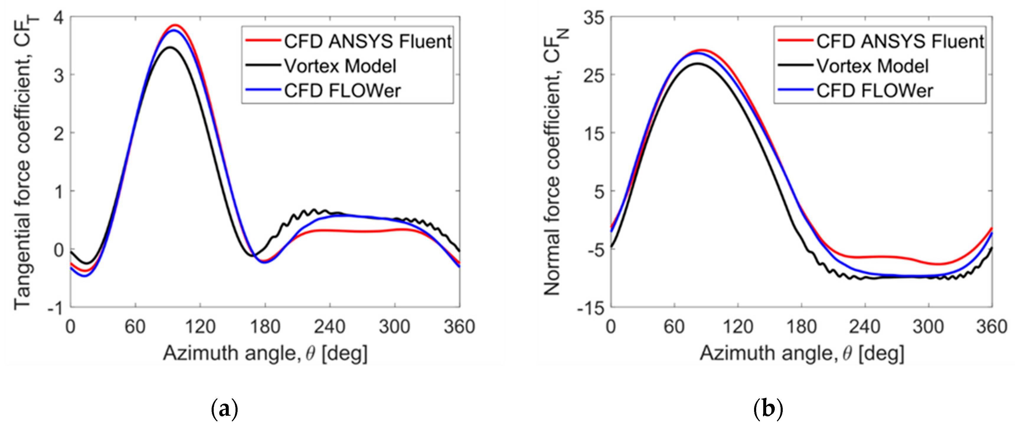
4.2. Instantaneous Aerodynamic Blade Loads

All numerical results presented in this paper were computed using ANSYS Fluent, Release 17.1 solver and the unsteady RANS (URANS) method with the SST k-ω turbulence model. For the comparison, the aerodynamic blade loads were also computed using the CFD code FLOWer from German Aerospace Center that was continuously extended for wind energy applications at IAG [67] and a vortex model from Technical University of Denmark (DTU).
The FLOWer code is a compressible code based on a fully structured mesh approach. Therefore, a different mesh was adopted in the calculations, employing an overset (Chimera) grid technique. This enables the user to build high quality meshes of each component independently. Further information about the mesh strategy and its topology is given in Bangga et al. [10]. The mesh of the rotor blade is resolved by 320 grid cells in the circumferential direction and by 32 cells across the boundary layer with a growth rate of 1.17, while maintaining the non-dimensional wall distance of y+ < 1.0. This mesh component is combined with fully structured Cartesian background meshes having a grid cell size of 0.23 m (Δ ≈ 0.026·R) near the rotor, based on a grid study for wake flow statistics in Bangga et al. [10]. The computations were carried out assuming a fully turbulent boundary layer employing the Menter SST k-ω model, consistent with the simulations performed using ANSYS Fluent, Release 17.1.
The vortex method calculates the induction at the blade positions from the influence of the continuously developing wake vorticity using the Biot-Savart law. The strength of the instantaneous bound circulation was calculated from the local inflow and airfoil data using the Kutta-Joukowski theory. A new vortex released in every time step at the trailing edge ensures that the total circulation remains constant in time. The airfoil data were calculated using XFOIL and presented in Figure 8. However, the effect of decambering from the blades moving in a curve was estimated as approximately 1 degree using thin airfoil theory and effectively shifting the lift curve 1 degree to the left. No dynamic stall model was used here. In these investigations, the rotor operating at the tip speed ratio of 5 and equipped with NACA 0018 airfoils was analyzed. The normal and tangential blade loads are shown in Figure 10. The two employed CFD codes and the vortex model deliver similar results of aerodynamic blade loads and, taken as verification that the equations, are solved correctly. However, some discrepancies are still observed in the predicted forces. FLOWer and Fluent deliver very similar predictions, while the forces obtained using the vortex method are slightly smaller. It shall be noted that the vortex method relies on the static polar data as its input. The results indicate the effects of Reynolds number variation over the azimuth and the rotor rotation on the blade boundary layer development. Despite that, the studies also demonstrate that all employed approaches are consistent for predicting the general characteristics of the rotor performance.

5. Results and Discussion

This section summarizes the results of studies on the aerodynamic performance of a Darrieus-type wind turbine. The first two subsections discuss the aerodynamic blade loads for symmetrical and cambered NACA airfoils. The last subsection describes aerodynamic wake downstream behind the rotor.

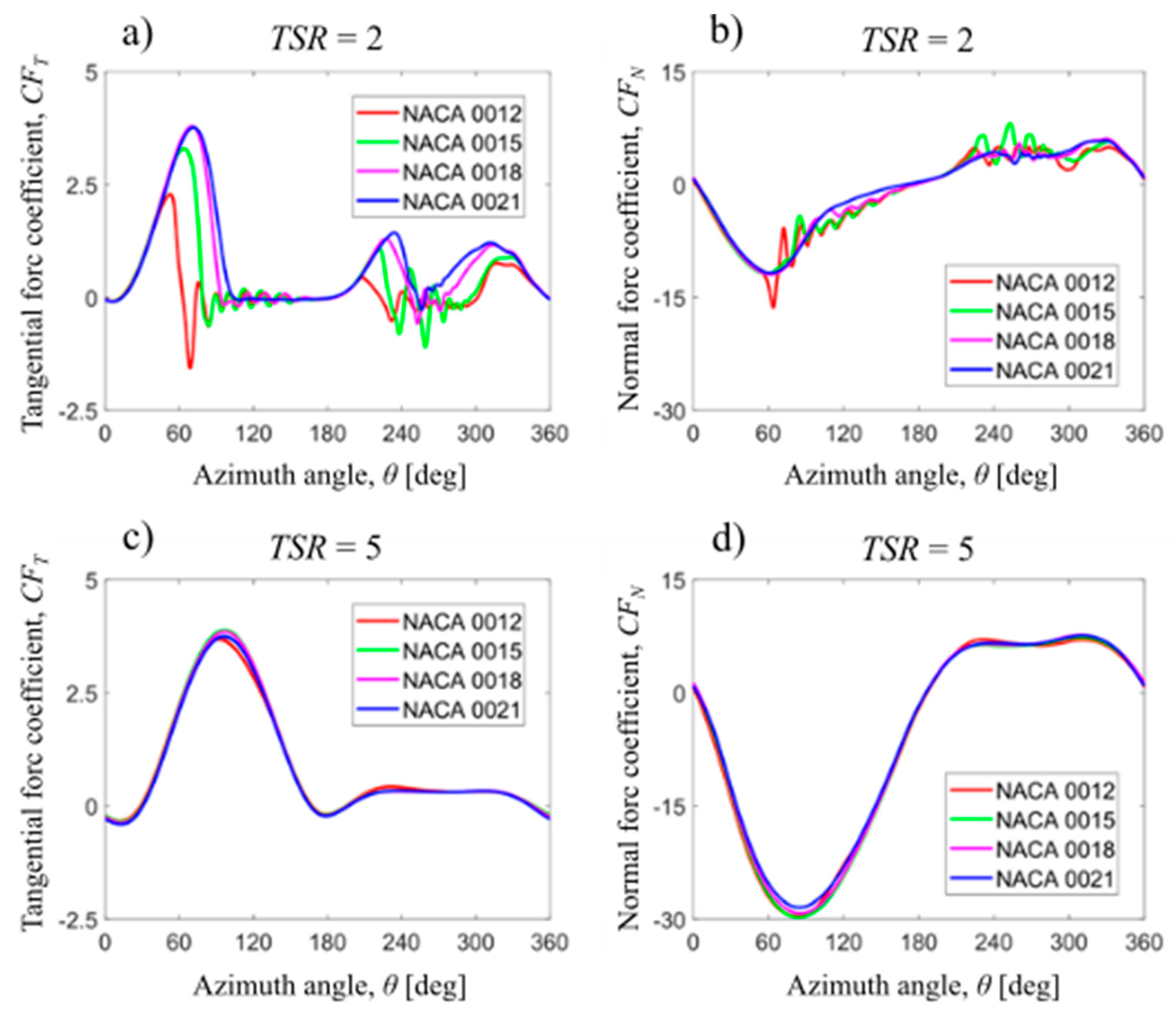
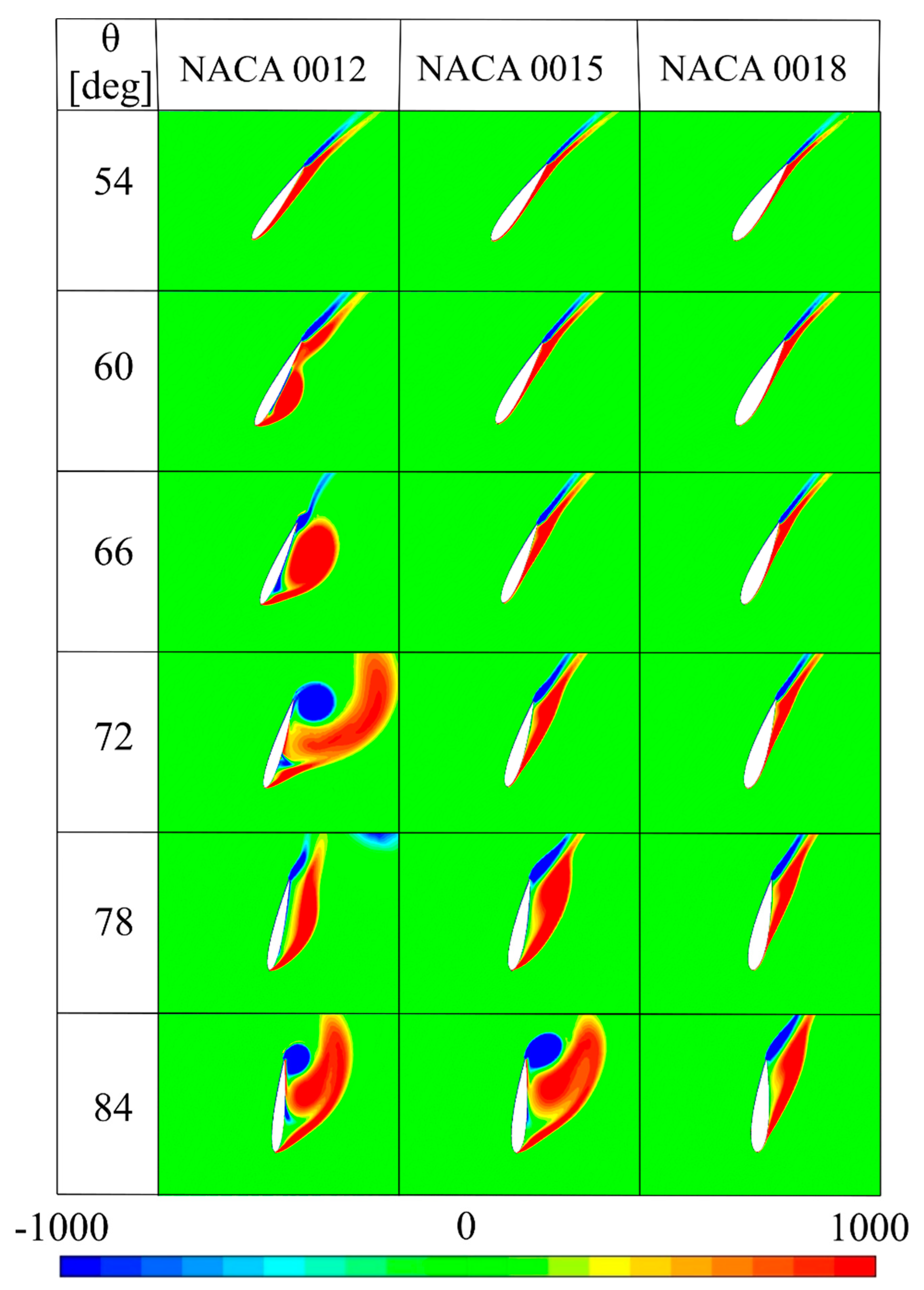
5.1. Aerodynamic Loads on a Rotor Blade for Symmetrical 4-Digit NACA Airfoils

Aerodynamic blade loads, tangential and normal components, depend on various aspects, such as, for example, tip speed ratio, rotor geometry, and Reynolds number. This paper only takes into account the influence of the airfoil shape and the tip speed ratio on aerodynamic blade loads. Figure 11 shows the distributions of the non-dimensionalized aerodynamic blade load components for two tip speed ratios: 2 and 5. The results are given for four symmetrical NACA airfoils from NACA 0012 to NACA 0021. This Figure 11 clearly shows that, in the case of symmetrical airfoils, the tip speed ratio has the greatest impact on the tangential blade load component. In the upwind part of the rotor, thinner airfoils show faster loss of tangential force with azimuth. In the case of the NACA 0012 airfoil, this decrease is already at θ = 52 degrees, causing the maximum value of this force coefficient to drop by almost 66% compared to the NACA 0018 airfoil. The early decrease in the tangential force in the case of thinner airfoils is related to the airfoil characteristics in vicinity of the critical angle of attack (the angle of attack that produces the maximum lift coefficient). Analyzing steady-state experimental data of lift coefficients of NACA 0012, NACA 0015, and NACA 0018 obtained by Sheldahl and Klimas [64] for Reynolds number of 1 × 10⁶, it can be stated that the airfoil with a relative thickness of 12% achieves the highest value of the maximum lifting force coefficient; however, the critical angle of attack is smaller compared to the NACA 0018 airfoil. If the blade pitch angle is zero, the geometric angle of attack is measured between the relative velocity and the wind velocity. At the tip speed ratio of 2, the azimuthal angle of 52 degrees corresponds to the local geometric angle of attack of 16.7 degrees. The effective angle of attack is of course lower than the geometric angle of attack because the flow velocity at the rotor is lower than the wind speed. However, this difference is not very large, especially in the upwind part of the rotor [1]. Therefore, for the NACA 0012 airfoil and at the azimuth of 52 degrees, flow detachment and consequent loss of lift may be expected. In addition, in the case of the NACA 0012 airfoil, the decrease in lift above the critical angle is much more rapid, indicating a leading edge stall, than in the case of NACA 0015 and NACA 0018 airfoils, for which the decrease in lift is much milder and where the separation starts at the trailing edge and gradually increasing with the angle of attack. It can also be seen from Figure 11 that the tangential blade load coefficient decreases rapidly in the downwind part of the rotor at azimuth around 200–235 degrees deepening on the relative thickness of the airfoil. In the case of low tip speed ratios, local angle of attack on both rotor sides exceeds critical values. Therefore, local decreases in tangential force observed in this part of the rotor result from exceeding the critical angle of attack. The differences between aerodynamic blade load coefficients for higher tip speed ratio of 5 are practically invisible to the naked eye. In general, all analyzed airfoils give an almost identical distribution of aerodynamic blade loads. However, a subtle difference can be seen for an azimuth of about 95 degrees, where the peak of the tangential blade load first increases with the thickness of the airfoil and then decreases. Song et al. [31], who also analyzed the aerodynamic performance of a Darrieus rotor with higher solidity and with symmetrical NACA 00XX airfoils, obtained a similar correlation. In the optimum tip speed ratio range, the maximum power coefficient was achieved by the rotor with NACA 0015 airfoils.
Figure 12 and Figure 13 show static pressure distributions around one rotor blade. The results are given for a rotor operating at a tip speed ratio of 2. Figure 12 presents the results for the NACA 0012 airfoil and Figure 13 for the NACA 0018. Figure 12 and Figure 13 show significant differences in pressure distributions for azimuth of 60 degrees. For the NACA 0012 airfoil, an anti-clockwise vortex is visible on the inside of the rotor blade. This vortex begins to form from an azimuth angle of 56–57 degrees. For θ = 60 degrees, it extends from the leading edge of the airfoil to about 2/3 of the chord length causing a local increase in flow velocity in the middle of the chord length, thus causing a loss of lift on the airfoil. This effect is not visible for the NACA 0018 airfoil.
Despite the use of URANS approach with the SST k-ω turbulence model, the oscillatory nature of the normal and tangential blade load components at TSR of 2 is observed in Figure 11. Choosing a fine time step size in URANS simulations allows for analysis of unsteady phenomena in the flow [9,10,13,19,26]. These phenomena in a low Reynolds number flow are mainly due to exceeding the critical angle of attack and the interaction of the blade aerodynamic wake with rotor blades. In the case of a wind turbine rotor at TSR of 2 with thinner airfoils (NACA 0012 and NACA 0015), the oscillatory nature of aerodynamic blade loads seems to be more visible in comparison with thicker airfoils (NACA 0018 and NACA 0021). As mentioned above, the NACA 0012 airfoil exhibits a sudden drop in the lift characteristic in comparison with thicker airfoils that show a smooth drop in the lift [64,68]. Moreover, the hysteretic behavior of the thick symmetrical NACA 00XX airfoils at stall is delated in comparison with thin profiles [69]. Therefore, aerodynamic wake downstream behind a thin airfoil at stall is thinner and tracking the development of this wake is easier with the URANS approach used than in the case of thick profiles. In addition, the static pressure distributions presented in Figs 12 and 13 given for the rotor operating at TSR of 2 show a greater tendency to form vortex structures on the edges of the NACA 0012 profile in the azimuth range of 60 to 180 degrees than the case of NACA 0018 airfoil.
Figure 14 presents vorticity fields around three profiles NACA 0012, NACA 0015, and NACA 0018 for the rotor operating at TSR of 2.
ω = ( v y x v x y ) e z ,
where vx and vy are flow velocity components. For better readability, the vorticity results were limited to a range from −1000 1/s to 1000 1/s. Red represents the anti-clockwise direction, and blue represents the clockwise direction. This figure clearly shows that, in the case of the NACA 0012 profile for θ = 54–60 degrees, a large anti-clockwise vortex appears on the leading edge. The same phenomenon also appears for the NACA 0015 airfoil, however, only on a smaller scale and for larger azimuths than in the case of the NACA 0012 airfoil.
The oscillatory nature of aerodynamic forces at low tip speed ratios may be related to the rotor solidity factor, σ. Rezaeiha et al. [70], who investigated the 1-m VAWT with the NACA 0018 airfoil, showed that the early drop in the instantaneous blade torque coefficient can be caused by lower solidity value of the Darrieus wind turbine rotor. The large rotor solidity can delay the early drop in aerodynamic blade loads. The wind turbine rotor investigated in this work has the rotor solidity of 0.2; however, the rotor size is much larger in comparison with the 1-m VAWT by Rezaeiha et al. [70]. Therefore, the aerodynamic interaction of other blades can have similar effects as for a smaller rotor with a low solidity.
From the developer’s point of view, the average tangential aerodynamic blade load component is much more interesting. For this purpose, a filled contour plot containing the isolines of the rotor power coefficient as a function of tip speed ratio and maximum airfoil thickness was created (Figure 15). This figure clearly shows that the optimal airfoil for the examined wind turbine is the NACA 0018 airfoil. It should be emphasized, however, that the area of the largest power coefficients (the area of CP around 0.5) for the NACA 0015 airfoil shifts towards higher tip speed ratios. Moreover, the thicker airfoil (NACA 0018) is slightly worse at a tip speed ratio of 6 than the NACA 0015 airfoil.

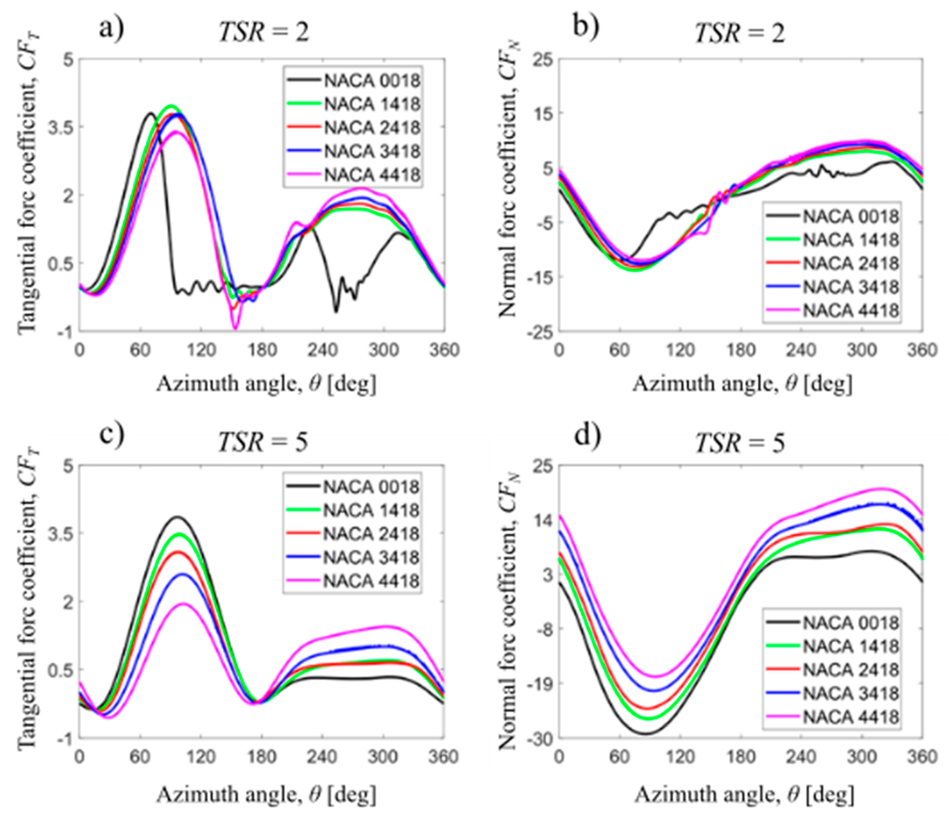
5.2. Aerodynamic Blade Loads for Cambered 4-Digit NACA Airfoils

The previous section discusses the impact of maximum airfoil thickness on rotor performance. Another very important parameter of NACA 4-digit airfoils is the maximum airfoil camber. The impact of this factor on rotor performance is discussed in this section.
Figure 16 illustrates the impact of the maximum camber on aerodynamic blade loads for two tip speed ratios, 2 and 5. Generally, as the power coefficient results presented in Figure 17 show, the airfoil with a small camber equal to 1% (NACA 1418) shows better performance over the entire analyzed tip speed ratio spectrum than the symmetrical airfoil NACA 0018. The shape of aerodynamic blade load components of curved airfoils is also different compared to symmetrical airfoils (Figure 16). This is most visible for tangential blade load component at a tip speed ratio of 2. Asymmetrical airfoils do not experience a sudden loss of tangential blade load for azimuths 70 degrees and 230 degrees. The increase in the maximum camber of the airfoil causes a decrease in the maximum tangential force on the upwind part of the rotor and an increase in the maximum tangential force on the downwind side. For the upwind part of the rotor, the maximum tangential blade load coefficient for the NACA 4418 airfoil is 15% lower compared to the NACA 1418 airfoil and 11% compared to the NACA 0018 airfoil. For the downwind part of the rotor, the maximum tangential blade load for the NACA 1418 airfoil is 21% lower compared to the NACA 4418 airfoil. The shape of the tangential blade load curves changes when the tangential blade velocity increases compared to the wind speed. Figure 16 shows the relationship of the tangential blade load component of the blade for a ratio of these velocities of 5. The results are given for five 4-digit NACA series airfoils. The differences in the maximum values of the tangential blade load coefficient for different NACA airfoils on both sides of the rotor are much larger than for the velocity ratio of 2. For the upwind part of the rotor, the maximum tangential blade load coefficient value for the NACA 4418 airfoil is 1.94 and is 49.5% lower compared to the NACA 0018 airfoil. In the case of the downwind part of the rotor, the maximum tangential load coefficient for the NACA 0018 airfoil is 0.32 and is 78% lower compared to the NACA 4418 airfoil. The change in the maximum values of the tangential blade load coefficient as a function of the maximum airfoil camber as percentage of the chord for the upwind part of the rotor is almost linear with the slope of −0.47. Interestingly, all CFT curves have the same value close to zero for an azimuth close to 180 degrees. This is the location where the chords of the airfoils are parallel to the wind direction and the wind blows from the back. All curves also have a very similar value of about −0.38 when the blade passes through an azimuth of 13 degrees. The ratio of the maximum values of the tangential blade load for the upwind part of the rotor to the maximum values of this load for the downwind part as a function of maximum airfoil camber can also be approximated by a straight line. This ratio reaches a value from 11.6 for the NACA 0018 airfoil to 1.34 for the NACA 4418 airfoil. Thus, for the airfoil with the largest maximum camber examined, the tangential blade load peak on both sides of the rotor area is almost equal. The decrease in the tangential blade load for the NACA 0018 airfoil (Figure 14) can also be caused by so-called virtual blade camber. It is caused by a curved flow field caused by the revolution of the wind turbine rotor. Airfoil characteristics are usually measured in a wind tunnel with straight flow field. The curved flow field causes the symmetrical airfoil of a vertical axis wind turbine to work as a cambered airfoil. This causes a change in the lift coefficient characteristics of the airfoil. For a given angle of attack, the value of the lift coefficient of the symmetrical airfoil with the “virtual camber” is lower compared to the symmetrical airfoil in straight flow field [71].
While comparing the distribution of the normal component of the aerodynamic blade load, it can be seen that the differences in these distributions increase with tip speed ratio. For a tip speed ratio of 2, CFN distributions for the different airfoils investigated are very similar, whereas, for a tip speed ratio of 5, the curves are very similar, but they are offset by almost constant value from one another. A detailed analysis of the normal component of the aerodynamic blade load for a tip speed ratio of 2 shows, however, that, as in the case of TSR = 5, the behavior of the curves is identical, the curve offset is also visible, although the value of the offset of the curves is very small. Only the curve corresponding to the NACA 0012 airfoil has a different shape from the others and as already described, it is associated with a sudden loss of lift on this profile. It can be seen that, in the 0–60-degree, 164–226-degree, and 314–360-degree azimuth ranges, the trends of both CFT and CFN for TSR = 2 are identical to those for TSR = 5. In the upwind part of the rotor, the absolute value of the maximum normal blade load coefficient decreases almost linearly with the maximum camber of the airfoil from 29.2 for the NACA 0018 airfoil to 17.7 for the NACA 4418 airfoil, whereas the CFNmax in the downwind part of the rotor increases almost linearly from 7.63 for the NACA 0018 airfoil to 20.13 for the NACA 4418 airfoil. The slopes of straight lines passing through CFNmax as a function of maximum airfoil camber are −2.865 for the upwind part of the rotor and 2.993 for the downwind part of the rotor. In the case of TSR = 2, the slopes are also very similar, at −0.591 for the upwind part of the rotor and 0.63 for the downwind part of the rotor; however, in the case of TSR = 2, the NACA 0018 profile was not used for the analysis. For TSR = 5, the ratio of maximum normal blade load coefficient in the upwind part of the rotor to the downwind part of the rotor is from 3.82 for the NACA 0018 airfoil to 0.88 for the NACA 4418 airfoil, while, for TSR = 2, this ratio is from 1.72 for the NACA 1418 airfoil to 1.2 for the NACA 4418 airfoil.

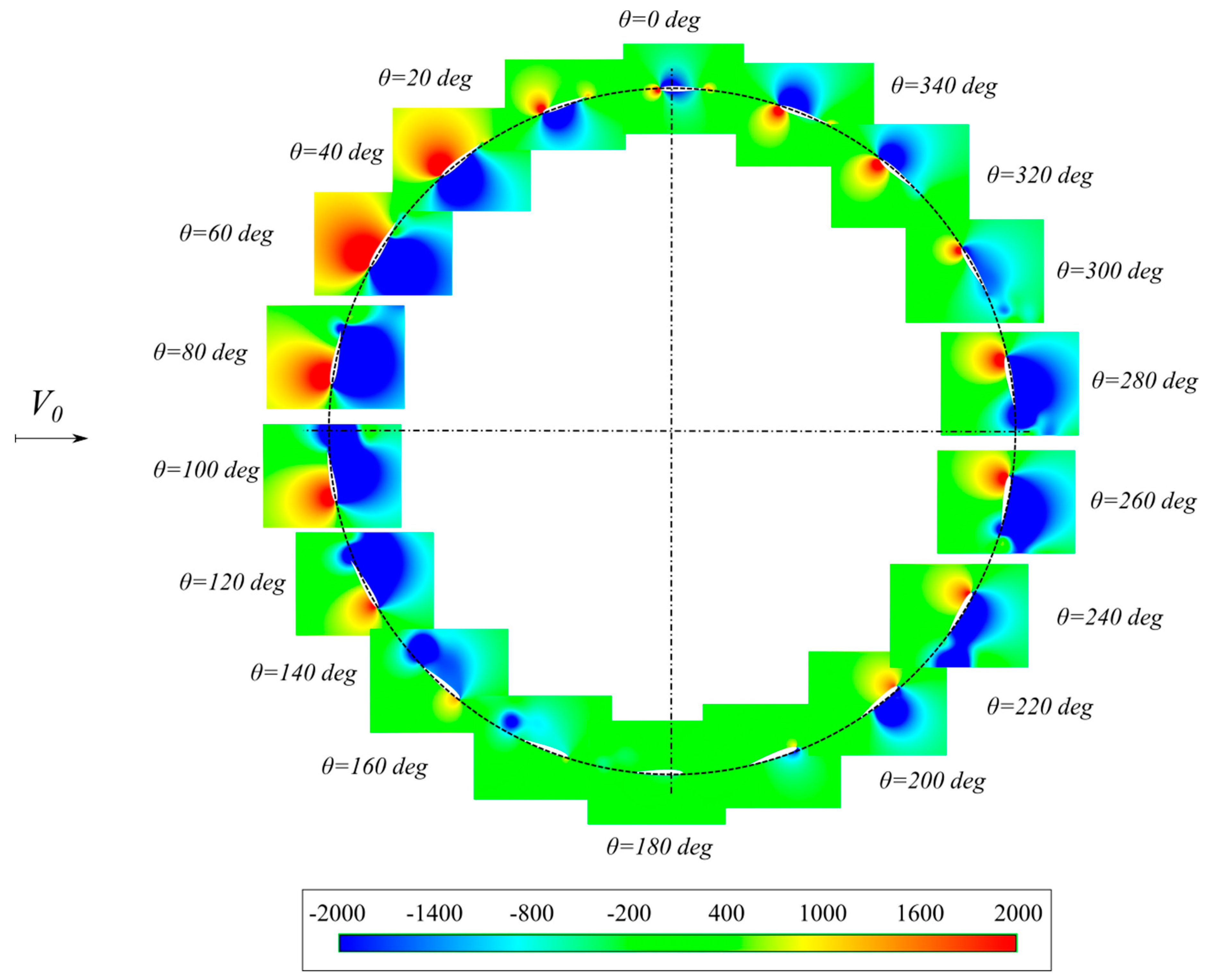
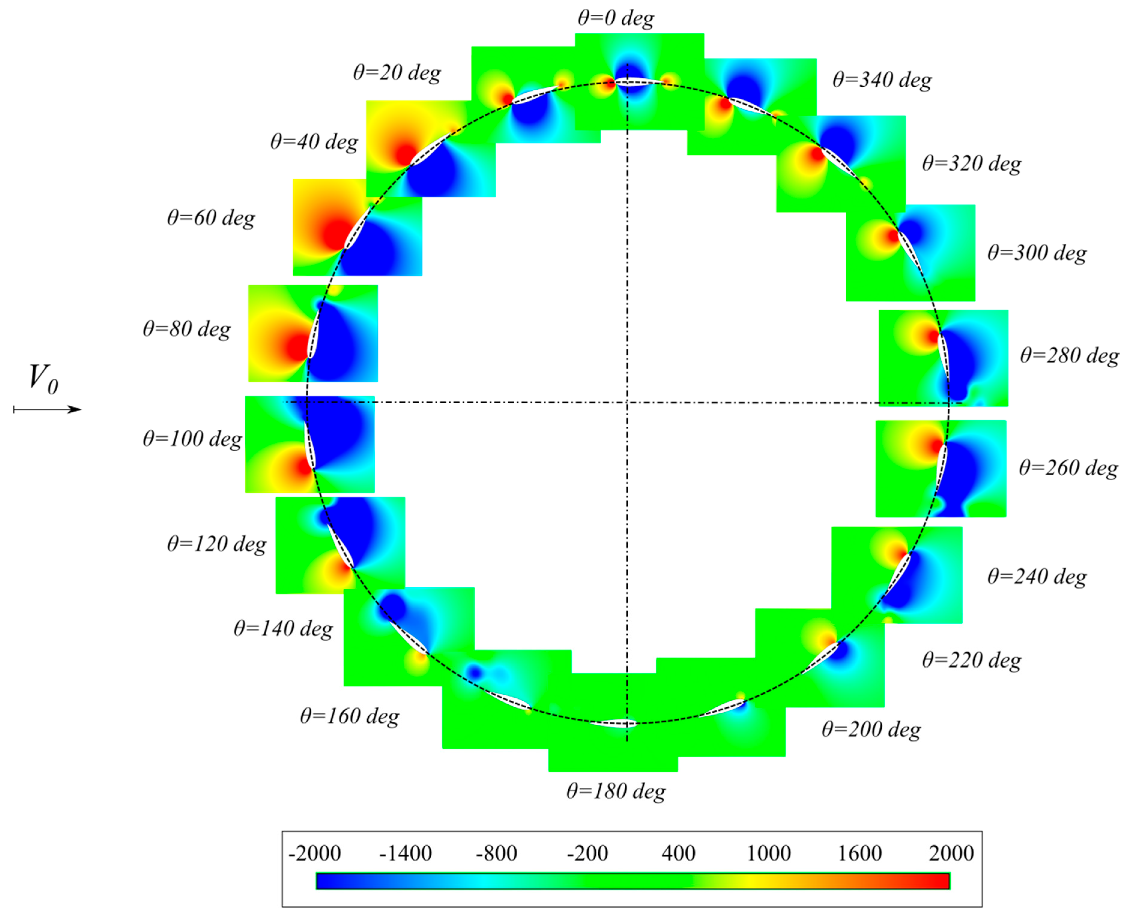
5.3. Aerodynamic Wake for Symmetrical and Cambered 4-Digit NACA Airfoils

The different shape of the aerodynamic blade loads described in the previous two subsections also affects the velocity distribution in the aerodynamic wake behind the rotor. This section deals with the impact of symmetrical airfoils on the air velocity field 1.5 R downstream, measured from rotor axis, of the rotor (Figure 4).
Figure 18 shows the impact of tip speed ratio on the distribution of two velocity components, Vx and Vy, downstream behind the rotor. Both velocity components are related to the wind velocity V0, while the coordinate y (please see Figure 4) is normalized by the radius of the rotor R. The velocity results presented in Figure 18 are given for the NACA 0018 airfoil. It is easy to see that the rotor has a greater effect on the velocity component Vx than on the component perpendicular to the wind direction Vy. As tip speed ratio increases, the velocity Vx decrease is larger. The average velocity of each of these profiles decreases almost linearly as a function of tip speed ratio from 0.92 for TSR = 2 to 0.57 for TSR = 6. It also seems that, except in the case of TSR = 2, the velocity component Vx profiles are almost symmetrical. In the case of velocity component Vy, its average for each tip speed ratio value is very close to zero. When analyzing the distribution of this velocity component, the more important factor visible to the naked eye is the slope of the function Vy / V0 (y / R). In this discussion, we have limited our considerations for the y / R ratio range from -1 to 1 because in this range the Vy/V0 curves are the most linear. For tip speed ratio 2, the curve slope d ( V y / V 0 ) / d ( y / R ) is small and is 0.014, whereas, for tip speed ratio 5, the slope is 0.0515. It is easy to see from Figure 16 that the change in the slope of these curves with tip speed ratio is not linear. In order to better illustrate this, a graph of the slope as a function of tip speed ratio was prepared (see Figure 19). From this figure, it can be seen that, as the tip speed ratio increases, the increase in slope is getting smaller.
Generally, as can be seen from Figure 18, the value of velocity component Vy is very small compared to the component Vx. The average value of velocity component Vy / V0 of all velocity profiles is 0.0028 and is smaller by about 99.6% compared to the average Vx / V0 of all velocity profiles. To better show the share of both components of velocity ratios, a vector graph of velocity ratio V/V0 was made for two tip speed ratios values, 2 and 6 (Figure 20). The speed V is defined as the root of the sum of the squares of the components Vx and Vy. The figure clearly shows that the velocity vectors for TSR = 6 are more deflected outwards at the coordinate | y / R | = 1.5 than in the case of TSR = 2.
Above, the influence of tip speed ratio on the distribution of velocity downstream behind the rotor has been described for NACA 0018 airfoil. Figure 21 shows the distribution of the velocity components Vx and Vy in the aerodynamic wake downstream behind the rotor for two tip speed ratios 3 and 6 depending on the relative thickness of the airfoil. Velocity distributions are given for four symmetrical airfoils: NACA 0012, NACA 0015, NACA 0018, and NACA 0021. This figure clearly shows that, except for the NACA0012 airfoil at the tip speed ratio of 3, the differences in the velocity profiles downstream behind the rotor, both the Vx and Vy components, are negligible. The average value of all velocity profiles Vx/V0 for TSR = 3 is 0.81 with a standard deviation of 0.014, whereas, in the case of the velocity profiles Vy/V0, the average value is −0.0049, with a standard deviation of 0.0023. For a tip speed ratio of 6, the average velocity of all Vx / V0 velocity profiles is 0.01173 with a standard deviation of 0.0117. The average value of the second velocity component for all Vy / V0 velocity profiles is 0.0004, with a standard deviation of 0.001. Based on the average velocity values and the standard deviation, it can be stated that the share of the velocity component parallel to the wind direction is larger than in the case of the velocity component Vy and that the differences in the velocity profiles downstream behind the rotor are lower in the case of the velocity component Vy.
Figure 22 presents the shapes of the velocity profiles downstream of the rotor depending on the maximum airfoil camber and tip speed ratio. The results are shown for three airfoils: NACA 0018, NACA 2418, and NACA 4418. Analyzing the velocity distributions shown in Figure 22, some similarities can be noticed between the curves for TSR = 3 and TSR = 6. The Vx / V0 curves seem to be very close to each other, while the Vy / V0 curves seem to be offset by some fixed value. Analyzing the average values and standard deviations, it can be seen that both in the case of the velocity component Vx and Vy, the differences between the results are very small, both for in the case of TSR = 3 and TSR = 6. For TSR = 3, the average velocity of all three Vx / V0 velocity profiles is 0.57 and the standard deviation is 0.007; the average velocity for all Vy velocity profiles is −0.007 with a standard deviation of 0.0068. In the case of TSR = 6, the average velocity of the three average Vy / V0 velocity profiles is 0.797 with the standard deviation equal to 0.0054, whereas, in the case of the second velocity component, the average velocity is −0.012, with standard deviation of 0.0052. The slopes of the Vy / V0 curves in the range of y / R from −1 to 1 are almost identical and are on average 0.037 for TSR = 3 and 0.05 for TSR = 6.

6. Conclusions

The purpose of these investigations was to analyze the impact of two parameters of 4-digit NACA series airfoils, maximum airfoil thickness and maximum camber on the aerodynamic blade load, on aerodynamic efficiency (maximum rotor power coefficient) of the H-Darrieus rotor and velocity distribution downstream behind the rotor. Both aerodynamic blade loads and velocity profiles downstream behind the rotor depend on these two geometrical airfoil parameters, as well a tip speed ratio. Different numerical methods of fluid dynamics were used in this work, and, for CFD, the k-ω SST turbulence model was utilized.
  • Steady-state simulations confirmed that the numerical model and computational mesh give reasonable results of aerodynamic force coefficients, lift, and drag components. ANSYS Fluent, Release 17.1 better predicts the relationship between lift and angle of attack, while XFoil gives a slightly better result of a minimum drag coefficient compared to the experiment. Other numerical codes, like FLOWer CFD and vortex model, have shown that ANSYS Fluent CFD code correctly estimates the unsteady blade load components of the wind turbine rotor.
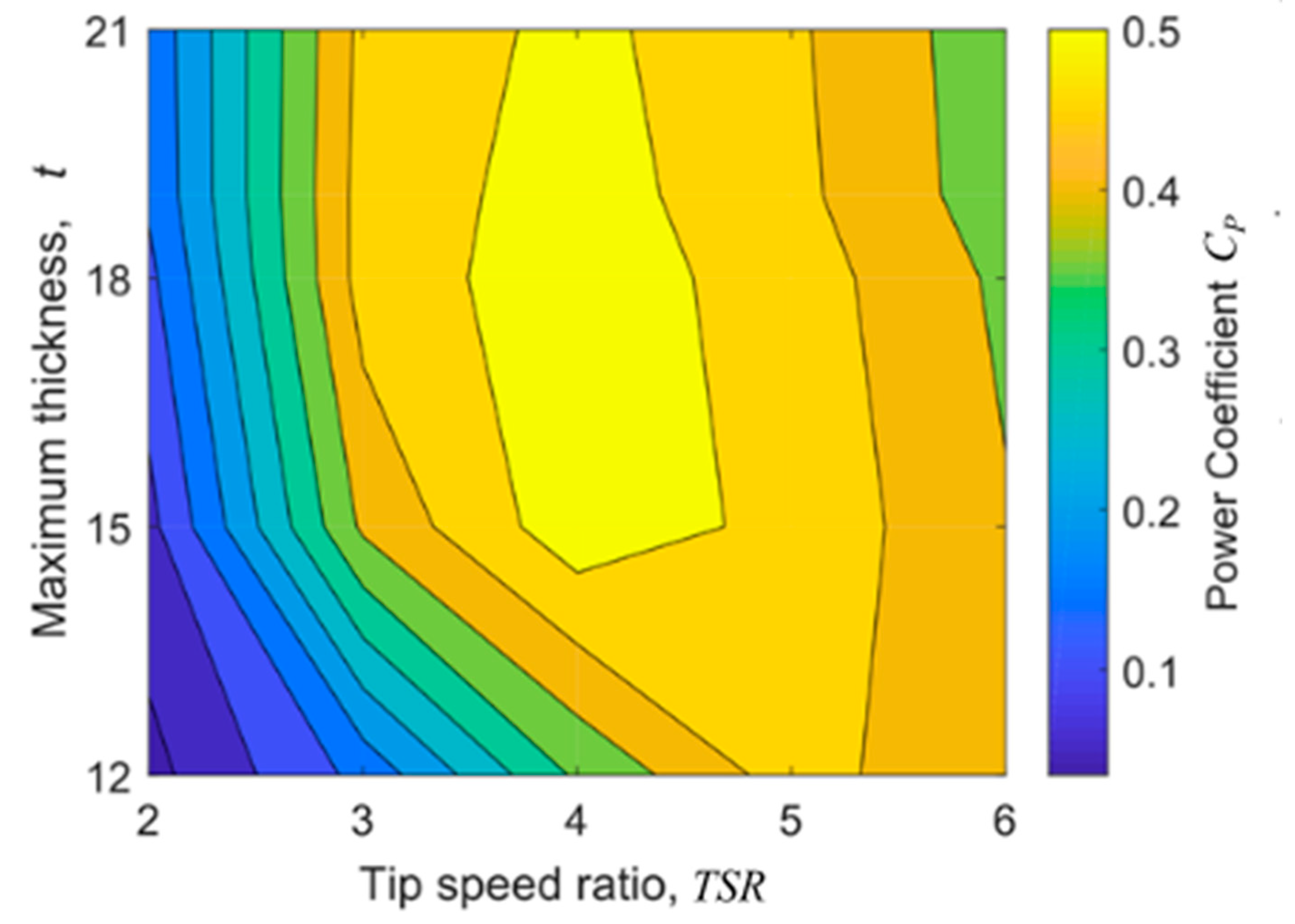
  • The first transient investigations concerned symmetrical airfoils from NACA 0012 to NACA 0021. When considering a wind turbine equipped with symmetrical NACA 0018 airfoils, the best aerodynamic performance was observed in the majority of tip speed ratio ranges.
  • Although the NACA 0012 airfoil has the largest maximum lift coefficient of all symmetrical airfoils tested, it gives the worst results of the tangential blade load in the low tip speed ratio range. This is due to the worse airfoil characteristics in the detachment area compared to thicker airfoils.
  • The analysis showed that symmetrical airfoils are much worse at low tip speed ratios. This is because of the worse characteristics of these airfoils in the stall regime. The introduction of one percent maximum camber greatly improves the aerodynamic performance of the rotor over the entire tip speed ratio range.
  • The effect of the relative airfoil thickness on the characteristics of aerodynamic blade load components is larger at low tip speed ratios, whereas the maximum camber affects more of these characteristics at higher tip speed ratios.
  • The use of cambered airfoils should improve the dynamic properties of the structure, e.g., reduce vibration. In the case of the NACA 4418 airfoil, the ratio of the maximum tangential blade load for the upwind part of the rotor to the downwind part is 88% lower compared to the NACA 0018 airfoil.
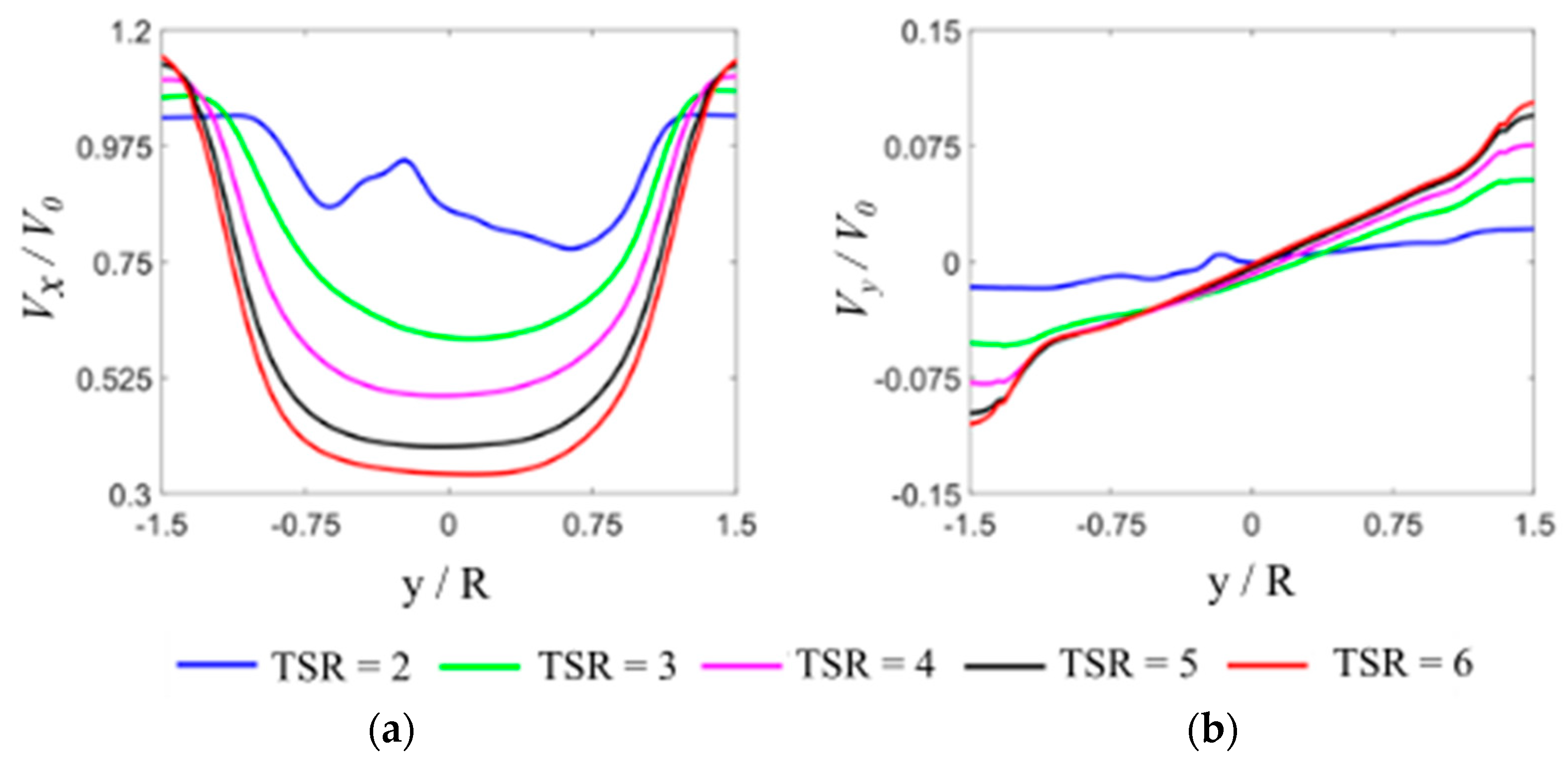
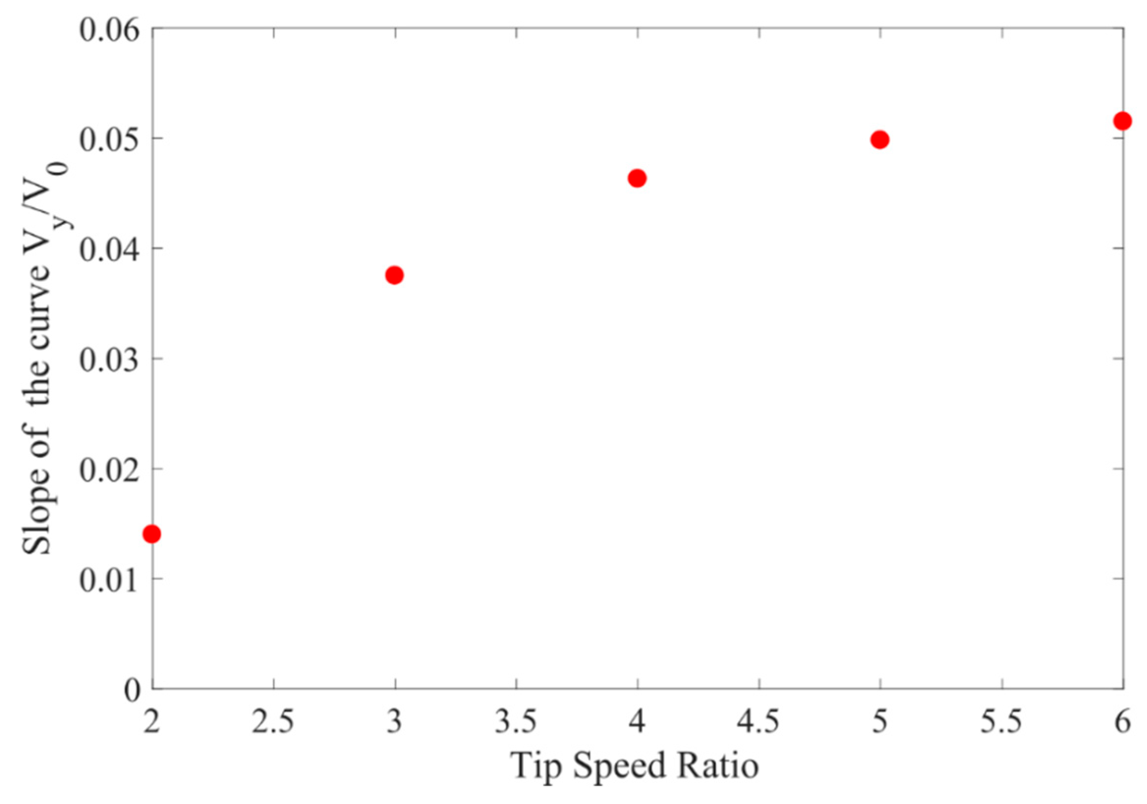
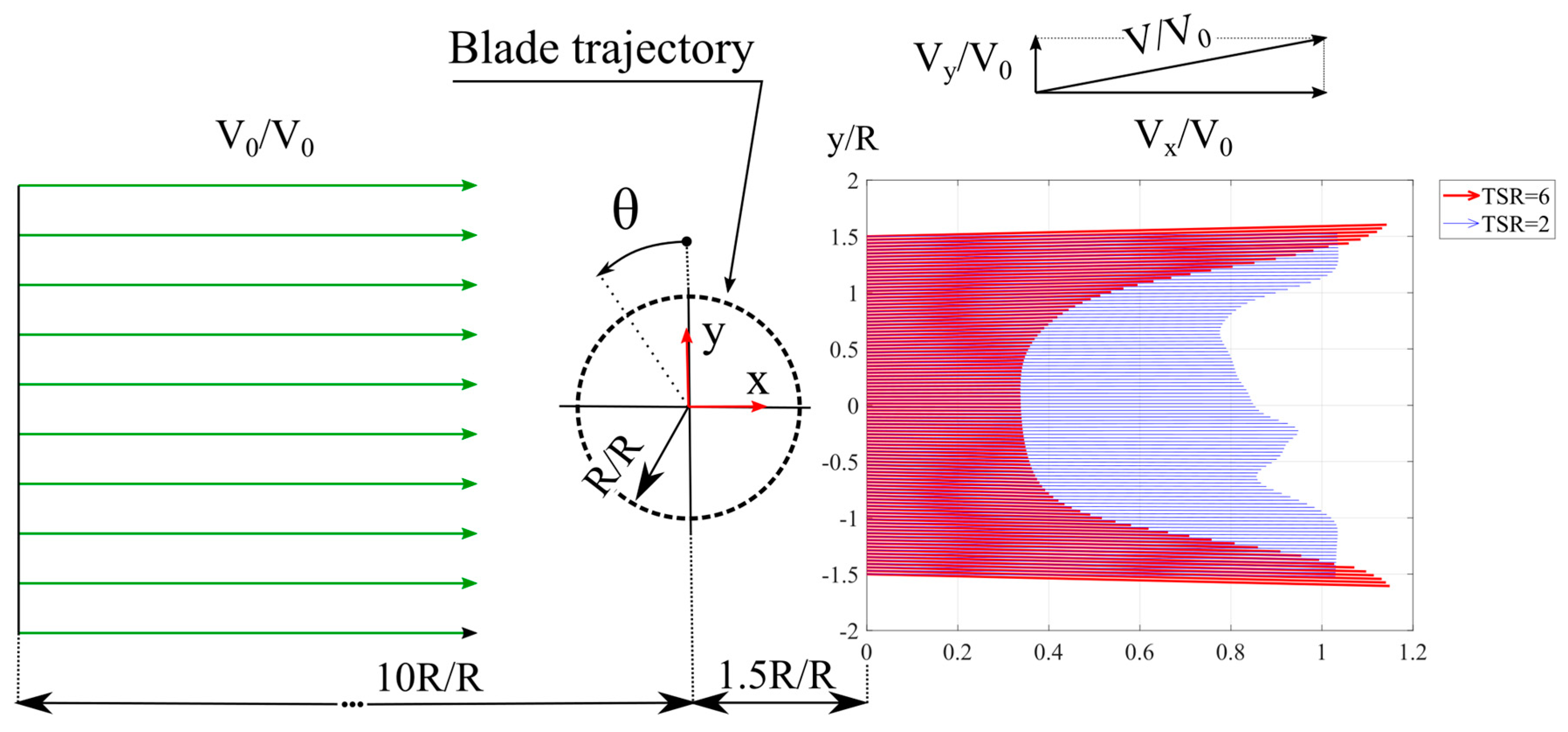
  • The study examined the impact of tip speed ratio on the velocity distribution in the aerodynamic wake of a rotor equipped with NACA 0018 airfoils. Numerical analysis showed that as the tip speed ratio increases, and there is a linear decrease in the average velocity Vx (velocity component parallel to the wind direction) of these profiles. In the case of the transverse velocity component Vy, its average for each tip speed ratio value is very close to zero. In the case of a rotor equipped with the symmetrical profile NACA 0018, it was observed that the share of the velocity component Vy in the aerodynamic shadow of the rotor is very low in the entire tested tip speed ratio range.
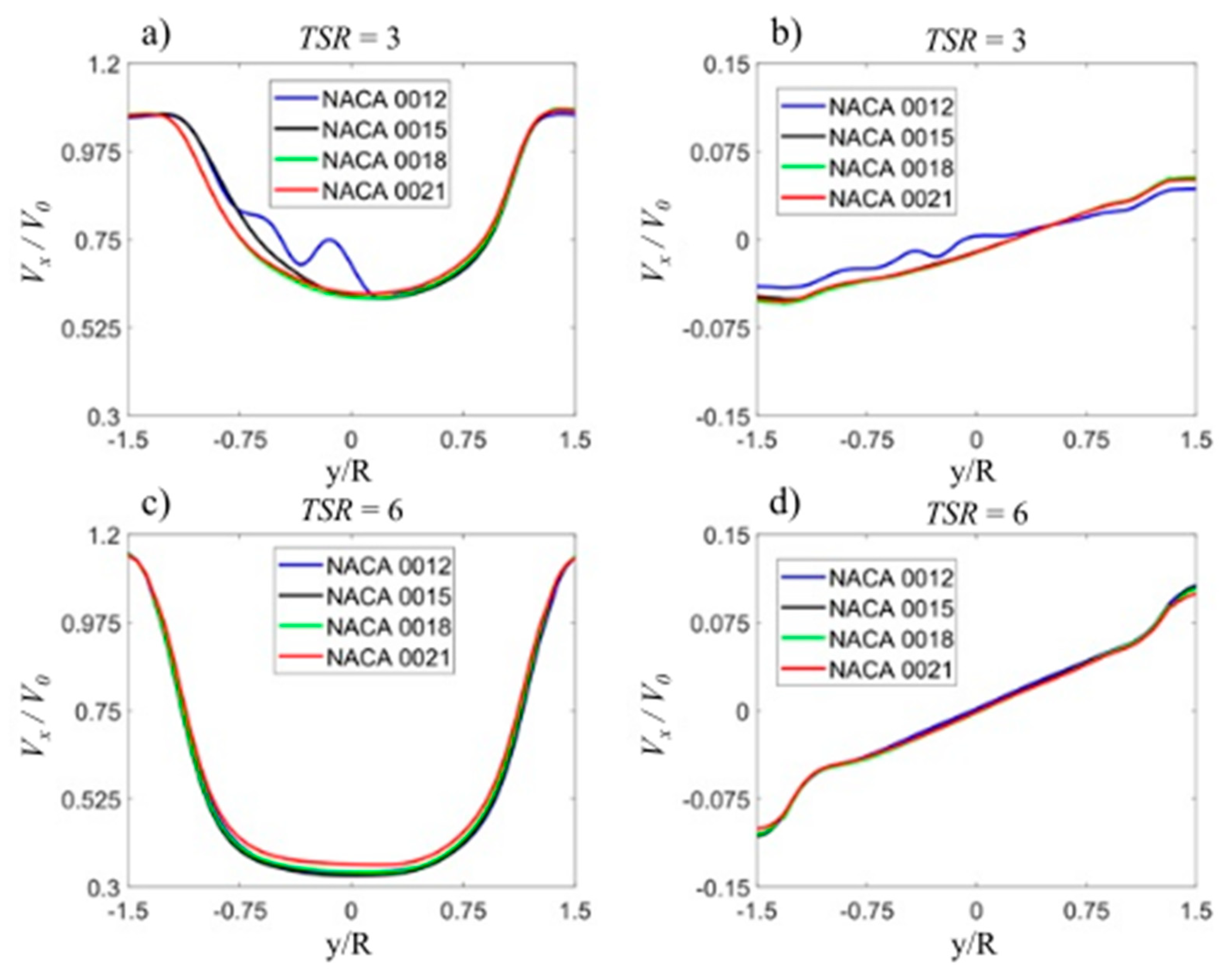
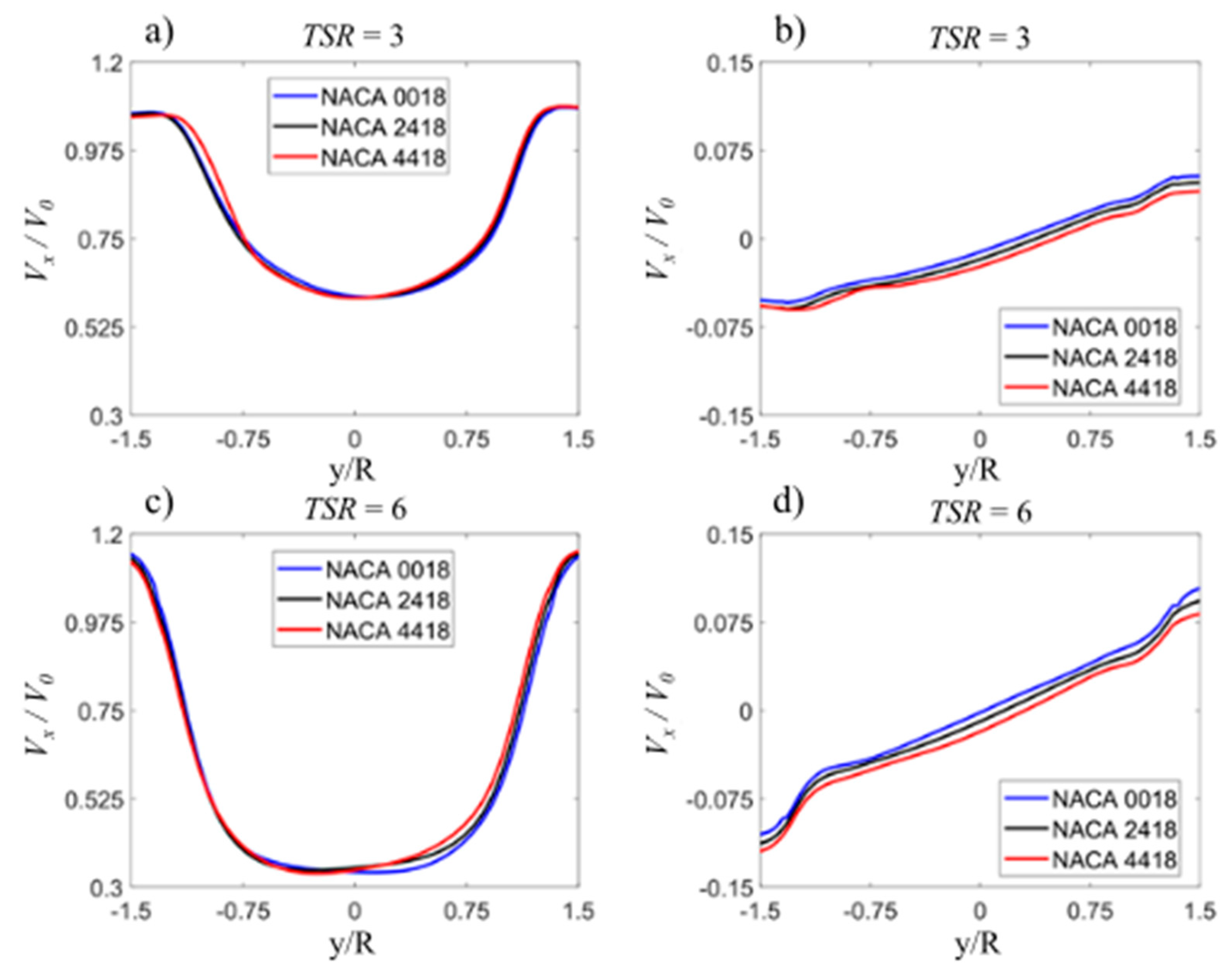
  • The increase in the relative thickness of symmetrical airfoils does not cause significant differences in the velocity distribution downstream behind the rotor in the entire investigated tip speed ratio range. The impact of maximum airfoil camber on the velocity distribution in aerodynamic shadow of the rotor is negligible. As in the case of symmetrical airfoils, the tip speed ratio has the biggest influence on the velocity distribution in the aerodynamic wake downstream behind the rotor.
  • Good experimental data is really missing to further validate the low TSR results. More investigation on the influence by the different turbulence models is needed in future work, especially naturally unsteady models, such as LES and detached eddy simulation (DES).

Author Contributions

K.R. performed the majority of the work including data analysis, along with writing of the manuscript.; M.O.L.H. supervised this work providing methodological guidance throughout the investigations. He also performed numerical analysis using the vortex model code and XFOIL code; moreover, he contributed to the writing of the manuscript.; G.B. supervised this work providing methodological guidance throughout the investigations. He also performed numerical analysis using CFD code FLOWer; moreover, he contributed to the writing of the manuscript. All authors have read and agreed to the published version of the manuscript.

Funding

This work was supported by National Science Centre, Poland, grant number 2018/02/X/ST3/03062, and the Interdisciplinary Center of Mathematical and Computer Modeling (ICM), grant number GB73-5.

Conflicts of Interest

The authors declare no conflicts of interest.

References

  1. Paraschivoiu, I. Wind Turbine Design: With Emphasis on Darrieus Concept; Presses Internationales Polytechnique: Montréal, QC, Canada, 2002. [Google Scholar]
  2. Anderson, J.W.; Brulle, R.V.; Bircheld, E.B.; Duwe, W.D. McDonnell 40-kW Giromill wind system: Phase I-Design and Analysis; Technical report; McDonnell Aircraft Company: St. Louis, MO, USA, 1979; Volume 2. [Google Scholar]
  3. Brulle, R. McDonnell 40-kW Giromill Wind System. Phase II. Fabrication and Test; Technical report; McDonnell Aircraft Co: St. Louis, MO, USA, 1980. [Google Scholar]
  4. Gipe, P. Wind Energy for the Rest of Us: A Comprehensive Guide to Wind Power and How to Use It; Wind-Works Org: Backersfield, CA, USA, 2016. [Google Scholar]
  5. Jankowski, K. Vertical Axis Wind Turbine of Darrieus H-Type with Variable Blade Incidence Angle Concept Design. Master’s Thesis, Warsaw University of Technology, Warsaw, Poland, 2009. [Google Scholar]
  6. Hansen, M. Aerodynamics of Wind Turbines, 3rd ed.; Earthscan: London, UK, 2015. [Google Scholar]
  7. Shamsoddin, S.; Porté-Agel, F. Large eddy simulation of vertical axis wind turbine wakes. Energies 2014, 7, 890–912. [Google Scholar] [CrossRef]
  8. Alaimo, A.; Esposito, A.; Messineo, A.; Orlando, C.; Tumino, D. 3D CFD analysis of vertical axis wind turbine. Energies 2015, 8, 3013–3033. [Google Scholar] [CrossRef] [Green Version]
  9. Bangga, G.; Hutomo, G.; Wiranegara, R.; Sasongko, H. Numerical study on a single bladed vertical axis wind turbine under dynamic stall. J. Mech. Sci. Technol. 2017, 31, 261–267. [Google Scholar] [CrossRef]
  10. Bangga, G.; Lutz, T.; Dessoky, A.; Krämer, E. Unsteady Navier-Stokes studies on loads, wake, and dynamic stall characteristics of a two-bladed vertical axis wind turbine. J. Renew. Sust. Energ. 2017, 9. [Google Scholar] [CrossRef] [Green Version]
  11. Li, Q.; Maeda, T.; Kamada, Y.; Hiromori, Y.; Nakai, A.; Kasuya, T. Study on stall behavior of a straight-bladed vertical axis wind turbine with numerical and experimental investigations. J. Wind. Eng. Ind. Aerodyn. 2017, 164, 1–12. [Google Scholar] [CrossRef]
  12. Rogowski, K.; Maroński, R.; Piechna, J. Numerical analysis of a small-size vertical-axis wind turbine performance and averaged flow parameters around the rotor. Arch. Mech. Eng. 2017, 64, 205–218. [Google Scholar] [CrossRef]
  13. Rogowski, K. Numerical studies on two turbulence models and a laminar model for aerodynamics of a vertical-axis wind turbine. J. Mech. Sci. Technol. 2018, 32, 2079–2088. [Google Scholar] [CrossRef]
  14. Rezaeiha, A.; Montazeri, H.; Blocken, B. Towards accurate CFD simulations of vertical axis wind turbines at different tip speed ratios and solidities: Guidelines for azimuthal increment, domain size and convergence. Energy Convers. Manag. 2018, 159, 301–316. [Google Scholar] [CrossRef]
  15. Wang, Y.; Shen, S.; Li, G.; Huang, D.; Zheng, Z. Investigation on aerodynamic performance of vertical axis wind turbine with different series airfoil shapes. Renew. Energy 2018, 126, 801–818. [Google Scholar] [CrossRef]
  16. Zhang, L.; Zhu, K.; Zhong, J.; Zhang, L.; Jiang, T.; Li, S.; Zhang, Z. Numerical investigations of the effects of the rotating shaft and optimization of urban vertical axis wind turbines. Energies 2018, 11, 1870. [Google Scholar] [CrossRef] [Green Version]
  17. Rezaeiha, A.; Montazeri, H.; Blocken, B. CFD analysis of dynamic stall on vertical axis wind turbines using scale adaptive simulation (SAS): Comparison against URANS and hybrid RANS/LES. Energy Convers. Manag. 2019, 196, 1282–1298. [Google Scholar] [CrossRef]
  18. Rezaeiha, A.; Montazeri, H.; Blocken, B. On the accuracy of turbulence models for CFD simulations of verticalaxis wind turbines. Energy 2019, 180, 838–857. [Google Scholar] [CrossRef]
  19. Rogowski, K. CFD Computation of the H-Darrieus wind turbine—The impact of the rotating shaft on the rotor performance. Energies 2019, 12, 2506. [Google Scholar] [CrossRef] [Green Version]
  20. Ishie, J.; Wang, K.; Ong, M.C. Structural dynamic analysis of semi-submersible floating vertical axis wind turbines. Energies 2016, 9, 1047. [Google Scholar] [CrossRef] [Green Version]
  21. Li, Q.; Kamada, Y.; Maeda, T.; Murata, J.; Okumura, Y. Fundamental study on aerodynamic force of floating offshore wind turbine with cyclic pitch mechanism. Energy 2016, 99, 20–31. [Google Scholar] [CrossRef]
  22. Bedon, G.; Schmidt Paulsen, U.; Aagaard Madsen, H.; Belloni, F.; Raciti Castelli, M.; Benini, E. Computational assessment of the DeepWind aerodynamic performance with different blade and airfoil configurations. Appl. Energy 2017, 185, 1100–1108. [Google Scholar] [CrossRef]
  23. Rossander, M.; Dyachuk, E.; Apelfröjd, S.; Trolin, K.; Goude, A.; Bernhoff, H.; Eriksson, S. Evaluation of a Blade Force Measurement System for a Vertical Axis Wind Turbine Using Load Cells. Energies 2015, 8, 5973–5996. [Google Scholar] [CrossRef] [Green Version]
  24. Bhutta, M.M.A.; Hayat, N.; Farooq, U.A.; Ali, A.; Jamil, S.R.; Hussain, Z. Vertical axis wind turbine—A review of various configurations and design techniques. Renew. Sust. Energ. Rev. 2012, 16, 1926–1939. [Google Scholar] [CrossRef]
  25. Möllerström, E.; Gipe, P.; Beurskens, J.; Ottermo, F. A historical review of vertical axis wind turbines rated 100 kW and above. Renew. Sust. Energ. Rev. 2019, 105, 1–13. [Google Scholar] [CrossRef]
  26. Rogowski, K.; Hansen, M.O.L.; Maroński, R.; Lichota, P. Scale adaptive simulation model for the darrieus wind turbine. J. Phys. Conf. Ser. 2016, 753, 022050. [Google Scholar] [CrossRef]
  27. Balduzzi, F.; Bianchini, A.; Maleci, R.; Ferrara, G.; Ferrari, L. Critical issues in the CFD simulation of Darrieus wind turbines. Renew. Energy 2016, 85, 419–435. [Google Scholar] [CrossRef]
  28. Healy, J.V. The influence of blade thickness on the output of vertical axis wind turbines. Wind Eng. 1978, 2, 1–9. [Google Scholar]
  29. Claessens, M.C. The Design and Testing of Airfoils for Application in Small Vertical Axis Wind Turbines. Master’s Thesis, Delft University of Technology, Delft, The Netherlands, 2006. [Google Scholar]
  30. Kirke, B.; Lazauskas, L. Enhancing the performance if a vertical axis wind turbine using a simple variable pitch system. Wind Eng. 1991, 15, 187–195. [Google Scholar]
  31. Song, C.; Wu, G.; Zhu, W.; Zhang, X. Study on aerodynamic characteristics of darrieus vertical axis wind turbines with diferent airfoil maximum thicknesses through computational fluid dynamics. Arab. J. Sci. Eng. 2020, 45, 689–698. [Google Scholar] [CrossRef]
  32. Danao, L.A.; Quin, N.; Howell, R. A numerical study of blade thickness and camber effects on vertical axis wind turbines. Proc. Inst. Mech. Eng. Part A J. Pow. Energy 2012, 226, 867–881. [Google Scholar] [CrossRef]
  33. Bianchini, A.; Balduzzi, F.; Ferrara, G.; Ferrari, L. Virtual incidence effect on rotating airfoils in Darrieus wind turbines. Energy Convers. Manag. 2016, 111, 329–338. [Google Scholar] [CrossRef]
  34. Sun, X.J.; Lu, Q.D.; Huang, D.G.; Wu, G.Q. Airfoil selection for a lift type vertical axis wind turbine. J. Eng. Thermophys. 2012, 33, 408–410. [Google Scholar]
  35. Moran, J. An Introduction to Theoretical and Computational Aerodynamics; Dover Publications INC: New York, NY, USA, 2003. [Google Scholar]
  36. Shires, A. Design optimisation of an offshore vertical axis wind turbine. Energy 2013, 166, 7–18. [Google Scholar] [CrossRef] [Green Version]
  37. Tjiu, W.; Marnoto, T.; Mat, S.; Ruslan, M.H.; Sopian, K. Darrieus vertical axis wind turbine for power generation I: Assessment of Darrieus VAWT configurations. Renew. Energy 2015, 75, 50–67. [Google Scholar] [CrossRef]
  38. Price, T.J. UK large-scale wind power programme from 1970 to 1990: The Carmarthen Bay experiments and the Musgrove vertical-axis turbines. Wind Eng. 2006, 30, 225–242. [Google Scholar] [CrossRef] [Green Version]
  39. Mays, I.D.; Morgan, C.A.; Anderson, M.B.; Powels, S.J.R. Experience with the VAWT 850 demonstration project. In Proceedings of the European Wind Energy Association Conference, Madrid, Spain, 10–14 September 1990. [Google Scholar]
  40. Apelfröjd, S.; Eriksson, S.; Bernhoff, H. A Review of Research on Large Scale Modern Vertical Axis Wind Turbines at Uppsala University. Energies 2016, 9, 570. [Google Scholar] [CrossRef] [Green Version]
  41. Ottermo, F.; Eriksson, S.; Bernhoff, H. Parking strategies for vertical axis wind turbines. ISRN Renewab. Energy 2012. [Google Scholar] [CrossRef] [Green Version]
  42. Templin, R. Design Characteristics of the 224 kW Magdalen Islands VAWT; National Research Council of Canada: Ottawa, ON, Canada, 1979. [Google Scholar]
  43. Zhong, J.; Li, J.; Guo, P.; Wang, Y. Dynamic stall control on a vertical axis wind turbine airfoil using leading-edge rod. Energy 2019, 174, 246–260. [Google Scholar] [CrossRef]
  44. Wong, H.K.; Chong, T.W.; Poh, S.C.; Shiah, Y.; Sukiman, N.L.; Wang, C. 3D CFD simulation and parametric study of a flat plate deflector for vertical axis wind turbine. Renew. Energy 2018, 129, 32–55. [Google Scholar] [CrossRef]
  45. Elsakka, M.M.; Ingham, D.D.; Ma, L.; Pourkashanian, M. CFD analysis of the angle of attack for a vertical axis wind turbine blade. Energy Convers. Manag. 2019, 182, 154–165. [Google Scholar] [CrossRef]
  46. Lichota, P.; Agudelo, D. A Priori Model Inclusion in the Multisine Maneuver Design. In Proceedings of the 17th IEE Carpathian Control Conference, Tatranska Lomnica, Slovakia, 29 May–1 June 2016. [Google Scholar] [CrossRef]
  47. Lichota, P.; Szulczyk, J.; Tischler, M.B.; Berger, T. Frequency Response Identification from Multi-Axis Maneuver with Simultaneous Multisine Inputs. J. Guid. Control. Dynam. 2019, 42, 2550–2556. [Google Scholar] [CrossRef]
  48. Bianchini, A.; Balduzzi, F.; Ferrara, G.; Ferrari, L.; Persico, G.; Dossena, V.; Battisti, L. Detailed analysis of the wake structure of a straight-blade H-Darrieus wind turbine by means of wind tunnel experiments and CFD simulations. In Proceedings of the ASME Turbo Expo 2017: Turbomachinery Technical Conference and Exposition, Charlotte, NC, USA, 26–30 June 2017. [Google Scholar] [CrossRef]
  49. Bianchini, A.; Balduzzi, F.; Rainbird, J.M.; Peiro, J.; Graham, J.M.R.; Ferrara, G.; Ferrari, L. An experimental and numerical assessment of airfoil polars for use in Darrieus wind turbines—Part I: Flow curvature effects. J. Eng. Gas. Turbine Pow. 2015, 138. [Google Scholar] [CrossRef]
  50. Bianchini, A.; Balduzzi, F.; Ferrari, L. Aerodynamics of Darrieus wind turbines airfoils: The impact of pitching moment. J. Eng. Gas. Turbine Pow. 2017, 139, 042602-1-12. [Google Scholar] [CrossRef]
  51. Mohamed, M.H.; Ali, A.M.; Hafiz, A.A. CFD analysis for H-rotor Darrieus turbine as a low speed wind energy converter. Eng. Sci. Technol. Int. J. 2015, 18, 1–13. [Google Scholar] [CrossRef] [Green Version]
  52. Hoerner, S.; Abbaszadeh, S.; Maître, T.; Cleynen, O.; Thévenin, D. Characteristics of the fluid–structure interaction within Darrieus water turbines with highly flexible blades. J. Fluid. Struct. 2019, 88, 13–30. [Google Scholar] [CrossRef] [Green Version]
  53. Ivanov, T.D.; Simonović, A.M.; Svorcan, J.S.; Peković, O.M. VAWT optimization using genetic algorithm and CST airfoil parameterization. FME Transact. 2017, 45, 26–32. [Google Scholar] [CrossRef] [Green Version]
  54. Tescione, G.; Ragni, D.; He, C.; Ferreira, C.S.; Van Bussel, G.J.W. Near wake flow analysis of a vertical axis wind turbine by stereoscopic particle image velocimetry. Renew. Energy 2014, 70, 47–61. [Google Scholar] [CrossRef]
  55. Tescione, G.; Ferreira, C.S.; Van Bussel, G.J.W. Analysis of a free vortex wake model for the study of the rotor and near wake flow of a vertical axis wind turbine. Renew. Energy 2016, 87, 552–563. [Google Scholar] [CrossRef]
  56. Beri, H.; Yao, Y. Effect of Camber Airfoil on Self Starting of Vertical Axis Wind Turbine. Environ. Sci. Technol. 2011, 4, 302–312. [Google Scholar] [CrossRef] [Green Version]
  57. Mohamed, M.H.; Janiga, G.; Pap, E.; Thévenin, D. Optimal blade shape of a modified Savonius turbine using an obstacle shielding the returning blade. Energy Convers. Manag. 2011, 52, 236–242. [Google Scholar] [CrossRef]
  58. Ferreira, C.J.S.; Van Zuijlen, A.; Bijl, H.; Van Bussel, G.; Van Kuik, G. Simulating dynamic stall in a two-dimensional vertical-axis wind turbine: Verification and validation with particle image velocimetry data. Wind Energy 2009, 13, 1–17. [Google Scholar] [CrossRef]
  59. Castelli, M.R.; Englaro, A.; Benini, E. The Darrieus wind turbine: Proposal for a new performance prediction model based on CFD. Energy 2011, 36, 4919–4934. [Google Scholar] [CrossRef]
  60. Trivellato, F.; Castelli, M.R. On the Courant-Friedrichs-Lewy criterion of rotating grids in 2D vertical-axis wind turbine analysis. Renew. Energy 2014, 62, 53–62. [Google Scholar] [CrossRef]
  61. Rogowski, K.; Hansen, M.O.L.; Lichota, P. 2-D CFD Computations of the two-bladed Darrieus-type wind turbine. J. Appl. Fluid Mech. 2018, 11, 835–845. [Google Scholar] [CrossRef]
  62. Rogowski, K.; Hansen, M.O.L. URANS and ACM for determining the aerodynamic performance of vertical-axis wind turbine. In E3S Web of Conferences; EDP Sciences: Les Ulis, France, 2019. [Google Scholar] [CrossRef] [Green Version]
  63. Menter, F. Two-equation Eddy-Viscosity turbulence models for engineering applications. AIAA J. 1994, 32, 1598–1605. [Google Scholar] [CrossRef] [Green Version]
  64. Sheldahl, R.E.; Klimas, P.C. Aerodynamic Characteristics of Seven Symmetrical Airfoil Sections Through 180-Degree Angle of Attack for Use in Aerodynamic Analysis of Vertical Axis Wind Turbines; Technical report SAND80-2114; Sandia National Labs: Albuquerque, NM, USA, 1981.
  65. Drela, M. XFOIL: An Analysis and Design System for Low Reynolds Number Airfoils. In Proceedings of the Conference on Low Reynolds Number Airfoil Aerodynamics, Notre Dame, IN, USA, 5–8 June 1989. [Google Scholar]
  66. Rezaeiha, A.; Kalkman, I.; Blocken, B. Effect of pitch angle on power performance and aerodynamics of a vertical axis wind turbine. Appl. Energy 2017, 197, 132–150. [Google Scholar] [CrossRef] [Green Version]
  67. Weihing, P.; Letzgus, J.; Bangga, G.; Lutz, T.; Krämer, E. Hybrid RANS/LES Capabilities of the Flow Solver FLOWer—Application to Flow Around Wind Turbines, Symposium on Hybrid RANS-LES Methods; Springer: Cham, Switzerland, 2016; pp. 369–380. [Google Scholar]
  68. Kumar, P.M.; Sivalingam, K.; Lim, T.C.; Ramakrishna, S.; Wei, H. Strategies for enhancing the low wind speed performance of H-DarrieusWind turbine—Part 1. Clean Technol. 2019, 1, 32–51. [Google Scholar] [CrossRef] [Green Version]
  69. Sarraf, C.; Djeridi, H.; Prothin, S.; Billard, J.Y. Thickness effect of NACA foils on hydrodynamic global parameters, boundary layer states and stall establishment. J. Fluids Struct. 2010, 26, 559–578. [Google Scholar] [CrossRef] [Green Version]
  70. Rezaeiha, A.; Montazeri, H.; Blocken, B. Towards optimal aerodynamic design of vertical axis wind turbines: Impact of solidity and number of blades. Energy 2018, 165, 1129–1148. [Google Scholar] [CrossRef]
  71. Akimoto, H.; Hara, Y.; Kawamura, T.; Nakamura, T.; Lee, Y.-S. A conformal mapping technique to correlate the rotating flow around a wing section of vertical axis wind turbine and an equivalent linear flow around a static wing. Lett. Environ. Res. Lett. 2013, 8. [Google Scholar] [CrossRef] [Green Version]
Figure 1. Silhouette of the McDonnell 40 kW. Photo by Paul Gipe. All rights reserved.
Energies 13 03196 g001
Figure 2. Four-digit NACA airfoils: (a) symmetrical NACA series; (b) cambered airfoils.
Energies 13 03196 g002
Figure 3. Velocity vectors, aerodynamic blade loads, and angles.
Energies 13 03196 g003
Figure 4. Numerical model, computational domain.
Energies 13 03196 g004
Figure 5. Computational mesh: (a) general view; (b) rotor area; (c) boundary layer mesh.
Energies 13 03196 g005
Figure 6. Mesh sensitivity test, rotor power coefficient versus number of mesh elements.
Energies 13 03196 g006
Figure 7. Initial condition effect, rotor torque coefficient as a function of time.
Energies 13 03196 g007
Figure 8. Aerodynamic airfoil characteristics: (a) lift coefficient; (b) drag coefficient. The comparison of CFD results with the experiment by Sheldahl and Klimas [64] and with the XFOIL predictions.
Energies 13 03196 g008
Figure 9. Aerodynamic airfoil characteristics of NACA 0012, NACA 0015, and NACA 0018: (a) lift coefficient; (b) drag coefficient. The comparison of CFD results with the experiment by Sheldahl and Klimas [64].
Energies 13 03196 g009
Figure 10. Aerodynamic blade load components: (a) tangential component; (b) normal component. Comparison of numerical results obtained with three different independent aerodynamic codes.
Energies 13 03196 g010
Figure 11. Aerodynamic blade load components for different maximum thickness of the NACA 4-digit airfoil: (a) and (b) present tangential and normal components, respectively at TSR of 2.0 whereas (c) and (d) at TSR of 5.0.
Energies 13 03196 g011
Figure 12. Static pressure (in Pascal) around the NACA 0012 airfoil at the rotor tip speed ratio of 2.
Energies 13 03196 g012
Figure 13. Static pressure (in Pascal) around the NACA 0018 airfoil at the rotor tip speed ratio of 2.
Energies 13 03196 g013
Figure 14. Vorticity fields, ω [1/s] around three NACA airfoil at six azimuthal positions.
Energies 13 03196 g014
Figure 15. Rotor power coefficient as a function of maximum airfoil thickness and tip speed ratio.
Energies 13 03196 g015
Figure 16. Aerodynamic blade load components, tangential component (on the left) and normal component (on the right), for different maximum camber of the NACA 4-digit airfoil and for two tip speed ratios, 2 and 5. Aerodynamic blade load components for different maximum camber of the NACA 4-digit airfoil: (a) and (b) present tangential and normal components, respectively at TSR of 2.0 whereas (c) and (d) at TSR of 5.0.
Energies 13 03196 g016
Figure 17. Rotor power coefficient as a function of maximum airfoil camber and tip speed ratio for t/c = 10%.
Energies 13 03196 g017
Figure 18. Velocity profiles downstream behind the rotor at the distance of 1.5 R form the rotor axis of rotation: (a) velocity component parallel to the wind direction, Vx; (b) perpendicular to the wind direction. The results are given for the NACA 0018 airfoil and for five tip speed ratios. Velocities Vx and Vy are normalized by wind speed V0.
Energies 13 03196 g018
Figure 19. The slope of the Vy/V0 function relative to y/R depending on the tip speed ratio.
Energies 13 03196 g019
Figure 20. The effect of tip speed ratio on the Vy velocity component.
Energies 13 03196 g020
Figure 21. Velocity profiles downstream of the rotor at the distance of 1.5 R form the rotor axis; the maximum airfoil thickness effect: (a) and (b) velocity component parallel to the wind direction, Vx, and velocity component perpendicular to the wind direction Vy, respectively at TSR = 3 whereas (c) and (d) at TSR = 6.
Energies 13 03196 g021
Figure 22. Velocity profiles downstream of the rotor at the distance of 1.5 R form the rotor axis; the maximum airfoil camber effect: (a) and (b) velocity component parallel to the wind direction, Vx, and velocity component perpendicular to the wind direction Vy, respectively at TSR = 3 whereas (c) and (d) at TSR = 6.
Energies 13 03196 g022
Table 1. Basic geometric parameters of the wind turbine.
ParameterValue
Rotor radius, R8.84 [m]
Blade length12.9 [m]
Chord, c0.61 [m]
Airfoil typeNACA 0018
Number of blades, B3
Rotor solidity, σ = Bc/R0.2

