Direct Power Control of a Single Stage Current Source Inverter Grid-Tied PV System

Abstract

In this paper, a direct power predictive controller (DPPC) is derived for a current source inverter (CSI) based single stage photovoltaic (PV) system. The equations of the dynamics, including AC and DC filters, are formulated directly for the PV power and for the active and reactive power injected in the grid. Then, the prediction equations are synthesized straight for the power, and, at each time instant, the optimal switching vector that guarantees simultaneously the control of the power generated by the PV arrays, and the control of the reactive power in the connection to the grid is chosen. This approach aims to guarantee fast and accurate tracking of the power. The proposed system is then validated through simulation and experimental results, showing that the PV system is able to follow the power references, guaranteeing a fast response to a step in the power, and decoupled active and reactive power control, with minimum total harmonic distortion (<5%) of the currents injected in the grid.

1. Introduction

The requirements of decarbonization are leading to the massive integration of renewable energies in the grid [1,2]. In particular, photovoltaic (PV) systems are becoming increasingly popular, used both for domestic and industrial applications with an average annual growth rate of 60% [3].

Grid-connected PV inverters are required to deploy energy directly to the grid and they are usually connected to the low voltage (LV) or medium voltage (MV) distribution grid [4,5]. International standards regulate power quality in the connection of PV inverters to the grid, bounding the harmonic content of the injected currents and setting limits to power factor regulation. IEEE standard (Std) 1547-2018 [6] provides a set of requirements for interconnection and interoperability of distributed resources with power system interfaces; IEC 61000-3-2 [7] sets limits for current harmonic emissions; IEEE Std 519-2014 [8] recommends practices and requirements for harmonic control in electric power systems with a set of recommended limitations for voltage and current harmonics; and IEC 61727 [9] lays down a set of requirements for the interconnection of PV systems to the distribution grid. Two of the most important impositions of these standards is the bounding of the total harmonic distortion (THD) of the injected currents, up to the 50th harmonic, to around 5%, and setting the minimum power factor to P_Fmin = 0.9 (inductive or capacitive) [10]. Beyond these international standards, additional grid codes apply in some countries, demanding higher flexibility [11] from grid-connected PV inverters. These requirements may range from mandatory galvanic isolation to low voltage ride through capabilities [3,12]. However, in recent years, efforts were made so that distributed renewable systems not only comply with international standards, but also actively contribute to minimize power quality issues in the connection to the grid, dynamically stabilizing the grid voltage and frequency, as in recent grid codes in Germany for PV power plants [4]. This can be achieved by means of active and reactive power control [13].

Regarding the topology selection, it is dependent on the installed power, on the PV system requirements, and on the application [3]. Some topologies make use of low frequency (LF) transformers, with obvious repercussions on the size and weight of the inverter [14]. This can be improved by the use of medium/high frequency transformers but still at the cost of efficiency. Therefore, focus was given on transformerless topologies [14,15], for which the downside is the absence of galvanic isolation [16]. Still, they present considerable advantages in terms of cost, efficiency, and volume, and are being increasingly used [16].

The most common transformerless solutions usually include a boost converter, followed by a voltage source inverter (VSI) in the connection to the grid [3]. The boost stage guarantees the maximum power point tracking (MPPT), maximizing the output power of the renewable resource, while the inverter stage injects the power to the grid. This solution has two conversion stages and a capacitive DC link between them, typically using electrolytic capacitors that are known to reduce the mean lifetime and eventually result in the failure of the converter [17].

Other transformerless solutions have been proposed [3], using single stage topologies, without the need for the capacitive decoupling stage, thus providing direct benefits on the cost, size, and lifetime of the inverter. The use of a single power stage can also potentially benefit efficiency, especially considering the expected proliferation of silicon carbide (SiC) and gallium nitride (GaN) semiconductors in power converters in future years [18], and their high efficiencies [19].

Research has been done on single stage converters for grid-connected PV inverters, both for single-phase and three-phase systems [20,21], with flexible power control capable of controlling the active power (P) and reactive power (Q) based on PQ theory [22].

Current source inverters (CSI) can be a strong candidate for single stage grid-connected PV systems, as they inherently behave as boost converters, allowing lower voltages on the arrays of panels. They do not require the use of electrolytic capacitors and the smooth DC side currents are a desirable feature for the PV panels [23]. Additionally, the expected evolution in reverse blocking semiconductors will lead to increased efficiency [24,25].

Grid-connected PV inverters using CSI topologies were explored in [26,27], where sliding mode controllers are used to directly control the current. In [26], active damping is used to further reduce the harmonic content of grid currents and minimize filter losses. Another example of a CSI topology, including an additional switch to attenuate the excitation of the LC filter, can be found in [28]. For this topology, a dedicated space vector modulation approach using the additional switch is synthesized.

In [23], two current control methods for a CSI based PV system are proposed to guarantee the MPPT and sinusoidal currents injected in the grid. The analysis is based on the model of the system dynamics, and the steady state and transient performance of the CSI based PV is tested under different fault conditions.

This paper proposes a direct predictive power controller (DPPC) based on model predictive control, a flexible and powerful approach to control power converters [29,30,31,32], from voltage source inverters in PV systems [33], to multilevel [34] or matrix converters [35,36,37], and also in drives [38], providing fast dynamic response and no steady-state error.

A DPPC is derived for a single stage PV system connected to the three-phase grid through a CSI. The main contribution of this paper is that the system model, including DC and AC filters, is directly obtained for the PV power and for the power injected in the grid, instead of being obtained for the state variables (inductor currents and capacitor voltages). Then, based on the equations of the power dynamics, the predictive controllers are synthesized to directly control the power in the PV and the reactive power in the connection to the grid. This is a novelty, as the usual approach is to control the AC inductor currents, which are state variables and are not exactly equal to the currents to be controlled (the grid currents). The dynamic response of the proposed DPPC is then experimentally evaluated under different operating conditions, and the power quality in the connection to the grid is assessed.

This paper is organized in five sections. In Section 2, the system is detailed and the model to characterize it is derived. In Section 3, the controller is synthesized, and in Section 4, the simulation and experimental results are obtained and compared. In Section 5, the main conclusions from the developed work are obtained and the main contributions of this work to the research field are summarized.

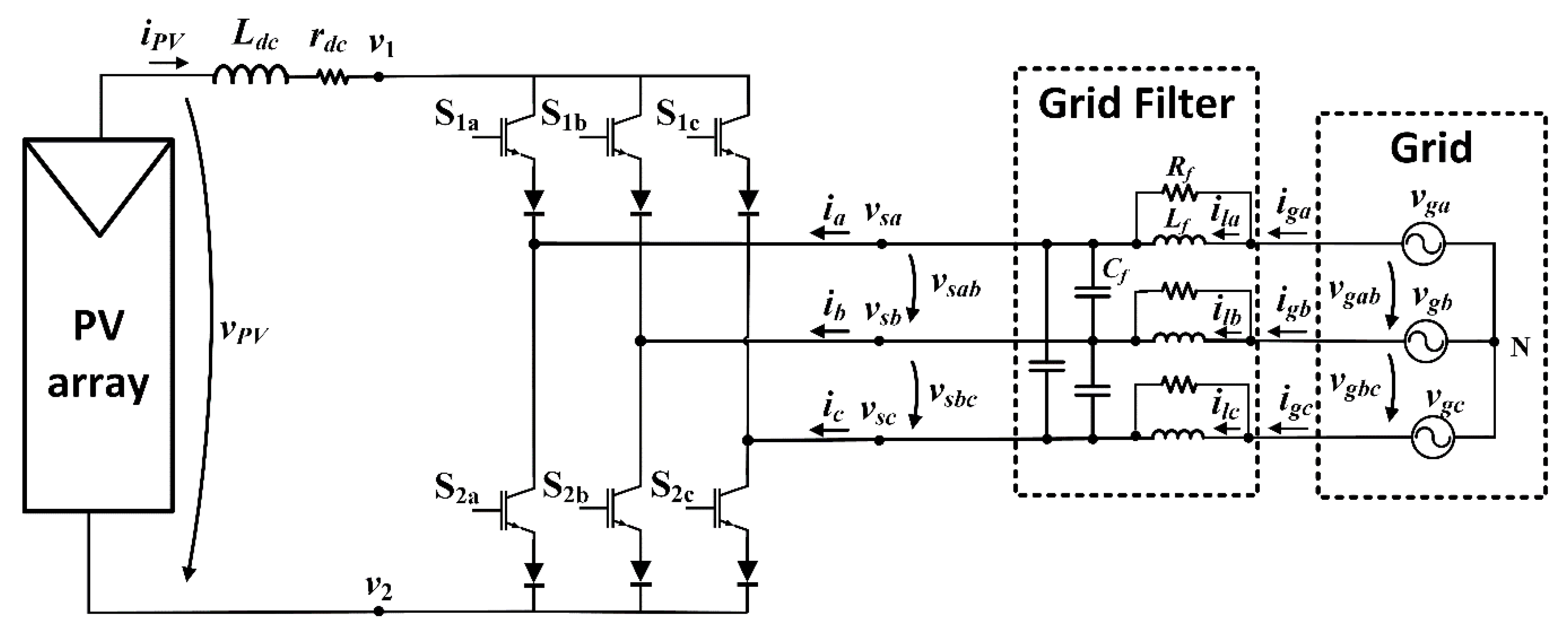
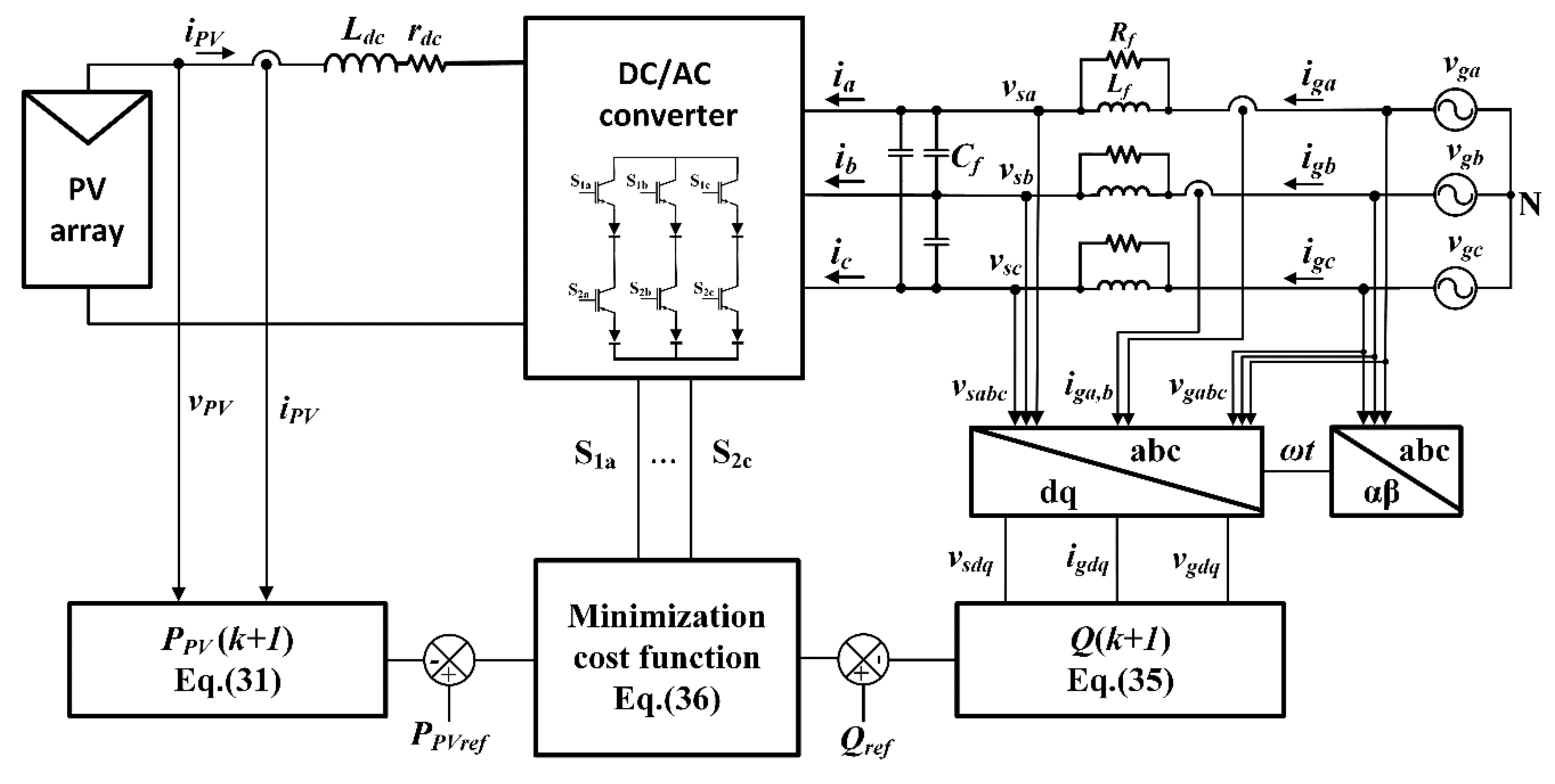
2. System Description

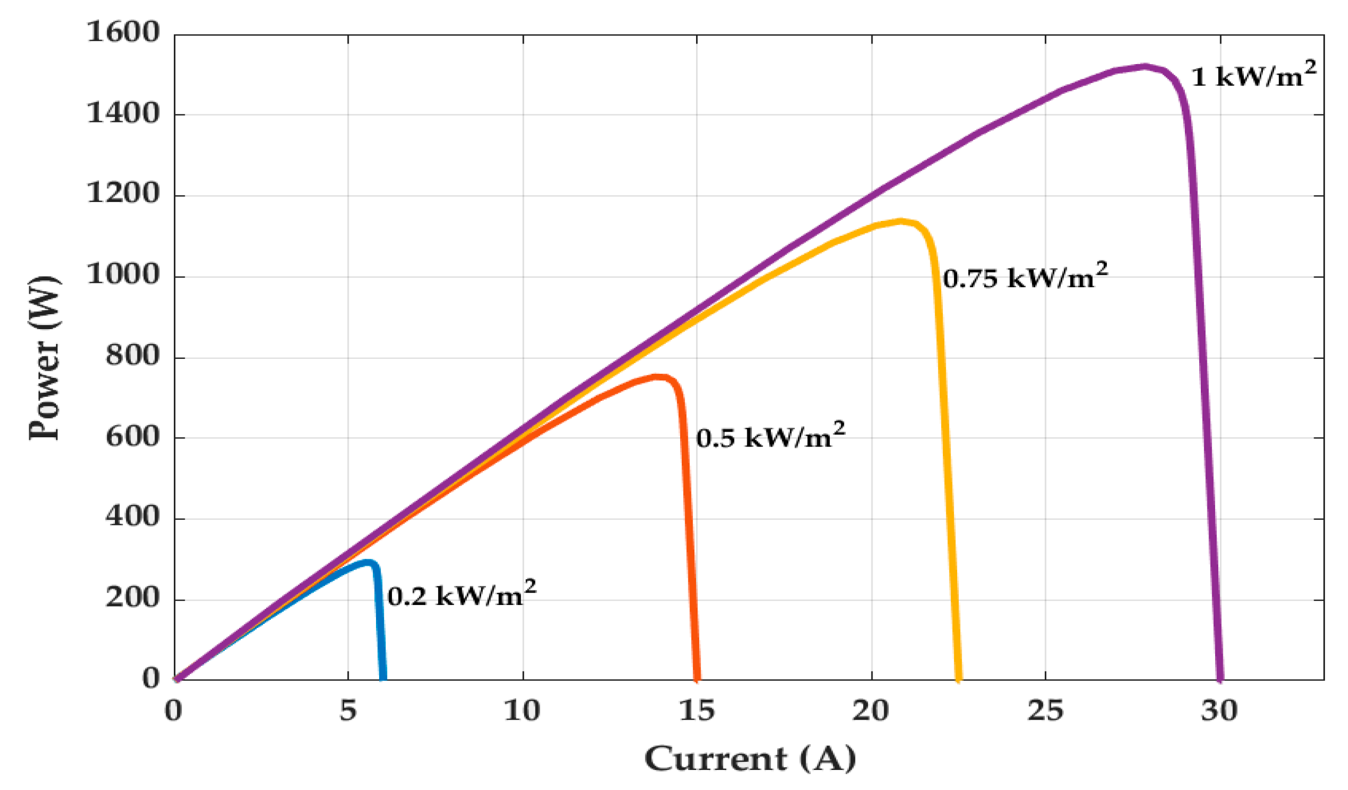
This section presents the model of the proposed system. The representation of the current source inverter (CSI), single stage three-phase grid-connected PV system is depicted in Figure 1. An approximate model of the PV array is used [39], being connected to the CSI through a filtering inductance L_dc (with parasitic resistance r_dc). Then, the CSI is connected to the grid through a second order LC filter [27,40] designed and sized to guarantee compliance with the IEEE 1547 standard, ensuring a displacement power factor higher than 0.9 in the connection to the grid, and a total harmonic distortion of the injected AC grid currents that is lower than 5% [27,41].

The model of the dynamics of the CSI based PV system is discussed in detail in the next sections.

2.1. PV Array Model

The PV array is modeled as shown in Figure 2, using the three parameters model representation [39], where i_ph is the photocurrent, dependent on the irradiation and temperature of the PV cell, and i_D is the diode current.

Considering the equivalent model of the PV cell presented in Figure 2, the PV current can be obtained from Equation (1),

$$i_{PV}=i_{ph}-i_D$$

(1)

The photocurrent (i_ph) of the PV cell changes with the irradiance level and cell temperature (T) according to Equation (2),

$$i_{ph}=\frac{G}{G_{ref}}\left(i_{sc}+{\mu }_T\left(T-T_{ref}\right)\right)$$

(2)

where i_sc is the short circuit current of the PV cell, G is irradiation level in kW/m², G_ref is the reference irradiation, 1 kW/m², and μ_T is the temperature coefficient of i_sc.

The diode current i_D represented in Figure 2 can be obtained from Equation (3),

$$i_D=i_o\left(e^{\frac{q{v}_{PV}}{mkT}}-1\right)$$

(3)

where i_o is the diode saturation current, q is the electric charge (1.6022 × 10⁻¹⁹ C), k is the Boltzmann’s constant (1.3806 × 10⁻²³ J/K), T is the cell temperature (K), and m is the diode quality factor (m = 1 for an ideal diode and m > 1 for a real diode).

The diode’s saturation current (i_o) changes with the cell temperature (T) and is expressed as in Equation (4):

$$i_o=i_o{}^r{\left(\frac{T}{T_{ref}}\right)}^3{e}^{\frac{\epsilon q}{mk{n}_s}\left(\frac{1}{T_{ref}}-\frac{1}{T}\right)}$$

(4)

where $i_o{}^r$ is the reference diode saturation current, $T_{ref}$ is the reference cell temperature and ε is the silica’s characteristic.

From Equation (1), the current of the PV cell, i_PV (Equation (5)) can then be expressed as a function of the cell’s voltage v_PV, considering the diode current i_D (Equation (3)), and an association of n_p paralleled PV modules, and n_s series-connected PV modules.

$$i_{PV}=n_p{i}_{ph}-n_p{i}_o\left(e^{\frac{q{v}_{PV}}{mkT{n}_s}}-1\right)$$

(5)

The PV data used in simulation, for the SunPower SPR305-WHT module, is presented in

Table 1. SunPower SPR305-WHT manufacturer data for the PV system.

Item	Value
Maximum Power, Pmax	305 W
Open circuit voltage, voc	64.2 V
Short circuit current, isc	5.96 A
Voltage at Pmax, vmpp	54.7 V
Current at Pmax, impp	5.58 A
Parallel strings, np	5
Series-connected modules per string, ns	1

.

The P–I characteristic of the PV is illustrated in Figure 3.

The power supplied by the PV can be obtained from Equation (6) by multiplying both sides of Equation (5) by v_PV:

$$P_{PV}=i_{PV}{v}_{PV}=v_{PV}{n}_p{i}_{ph}-v_{PV}{n}_p{i}_o\left(e^{\frac{q{v}_{PV}}{mkT{n}_s}}-1\right)$$

(6)

The power derivative can be calculated from Equation (7), and at maximum power $\frac{d{P}_{PV}}{d{v}_{PV}}=0$ [42]:

$$\frac{d{P}_{PV}}{d{v}_{PV}}=\frac{d\left(v_{PV}{i}_{PV}\right)}{d{v}_{PV}}=i_{PV}+v_{PV}\frac{d{i}_{PV}}{d{v}_{PV}}$$

(7)

The derivative of the PV power can also be obtained from Equation (8), considering the time derivative of the PV voltage and current. At maximum power $\frac{d{P}_{PV}}{dt}=0$ [42]:

$$\frac{d{P}_{PV}}{dt}=\frac{d\left(v_{PV}{i}_{PV}\right)}{dt}=i_{PV}\frac{d{v}_{PV}}{dt}+v_{PV}\frac{d{i}_{PV}}{dt}$$

(8)

The PV power dynamics will be computed using this equation.

2.2. Current Source Inverter Model

To reduce the number of conversion stages and avoid the use of a step-up transformer in the connection to the grid, a CSI is used to perform the DC to AC conversion, as depicted in Figure 1. Ideal switches are used to model the converter, containing three switches for each phase, where the ON/OFF state of each switch S_mn is defined as:

$$S_{mn}=\{\begin{array}{l}1,S_{mn}\mathrm{closed}\left(\mathrm{ON}\right)\\ 0,S_{mn}\mathrm{open}\left(\mathrm{OFF}\right),\end{array}\mathrm{where}m\in \left\{1,2\right\},n\in \left\{a,b,c\right\}$$

(9)

The states of CSI switches can be represented by matrix S:

$$S=\left[\begin{array}{l}\begin{array}{ccc}{S}_{1\mathrm{a}}& S_{1\mathrm{b}}& S_{1\mathrm{c}}\end{array}\\ \begin{array}{cc}\begin{array}{cc}{S}_{2\mathrm{a}}& S_{2\mathrm{b}}\end{array}& S_{2\mathrm{c}}\end{array}\end{array}\right],S_{ma}+S_{mb}+S_{mc}=1m\in \left\{1,2\right\}$$

(10)

To assure that the three-phase grid voltages are never short circuited and that the DC side inductive currents are never interrupted, the sum of all switch states connected to each output phase should be equal to 1 (Equation (10)). Considering this constraint, the switching states, output currents, and input voltage vectors of the CSI are presented in

Table 2. Switching states of CSI and corresponding PV side voltage and grid side currents of each state.

Vector	S1a	S1b	S1c	S2a	S2b	S2c	v12	isa	isb	isc
1	1	0	0	0	1	0	vab	iPV	−iPV	0
2	0	1	0	1	0	0	−vab	−iPV	iPV	0
3	0	1	0	0	0	1	vbc	0	iPV	−iPV
4	0	0	1	0	1	0	−vbc	0	−iPV	iPV
5	0	0	1	1	0	0	vca	−iPV	0	iPV
6	1	0	0	0	0	1	−vca	iPV	0	−iPV
7	1	0	0	1	0	0	0	0	0	0
8	0	1	0	0	1	0	0	0	0	0
9	0	0	1	0	0	1	0	0	0	0

.

Using the switching matrix S, the converter voltages (v₁, v₂) on the DC side and the grid side currents (i_a, i_b, i_c) can be obtained, respectively, from Equation (11):

$$\left[\begin{array}{l}{v}_1\\ v_2\end{array}\right]=S\left[\begin{array}{l}{v}_{sa}\\ v_{sb}\\ v_{sc}\end{array}\right],\left[\begin{array}{l}{i}_a\\ i_b\\ i_c\end{array}\right]=S^T\left[\begin{array}{c}-i_{PV}\\ i_{PV}\end{array}\right],$$

(11)

where (v_sa, v_sb, v_sc) are the converter grid side phase voltages and i_PV is the DC current. This equation will be further used to predict the future DC voltage of the converter (v₁₂) and the grid side currents.

2.3. Equations of PV Power Dynamics

The equation of the DC current (i_PV) dynamics (Equation (12)) is obtained by applying Kirchhoff’s laws to the circuit shown in Figure 1:

$$\frac{d{i}_{PV}}{dt}=\frac{v_{PV}-v_{12}}{L_{dc}}-\frac{r_{dc}}{L_{dc}}{i}_{PV},$$

(12)

where L_dc and r_dc represent the DC filtering inductance and its parasitic resistance, respectively. Using Equation (12) in Equation (8), the dynamics of PV power is obtained:

$$\frac{d{P}_{PV}}{dt}=-\frac{r_{dc}}{L_{dc}}{P}_{PV}+\frac{v_{PV}^2}{L_{dc}}-\frac{v_{12}}{L_{dc}}{v}_{PV}+i_{PV}\frac{d{v}_{PV}}{dt}$$

(13)

2.4. Equations of the Dynamics of Active and Reactive Power in the Connection to the Grid

Regarding the grid connection, the state variables, in abc coordinates, are the inductor currents (i_la, i_lb, i_lc) and the capacitor voltages (v_sab, v_sbc, v_sca).

The inductor currents (i_la, i_lb, i_lc) can be expressed as a function of the capacitors’ voltages (v_sab, v_sbc, v_sca) and the grid voltages (v_ga, v_gb, v_gc), and are obtained from Equation (14), where L_f represents the filter inductances [26,43].

$$\{\begin{array}{l}\frac{d{i}_{la}}{dt}=-\frac{2}{3L_f}{v}_{sab}-\frac{1}{3L_f}{v}_{sbc}+\frac{1}{L_f}{v}_{ga}\\ \frac{d{i}_{lb}}{dt}=-\frac{2}{3L_f}{v}_{sbc}-\frac{1}{3L_f}{v}_{sca}+\frac{1}{L_f}{v}_{gb}\\ \frac{d{i}_{lc}}{dt}=-\frac{1}{3L_f}{v}_{sab}-\frac{2}{3L_f}{v}_{sca}+\frac{1}{L_f}{v}_{gc}\end{array}$$

(14)

The dynamics of the capacitor’s voltages can be determined from Equation (15), where C_f represents the filter capacitance.

$$\{\begin{array}{l}\frac{d{v}_{sab}}{dt}=-\frac{2i_{gb}}{3C_f}-\frac{i_{gc}}{3C_f}+\frac{2i_b}{3C_f}+\frac{i_c}{3C_f}\\ \frac{d{v}_{sbc}}{dt}=-\frac{i_{ga}}{3C_f}-\frac{2i_{gc}}{3C_f}+\frac{i_a}{3C_f}+\frac{2i_c}{3C_f}\\ \frac{d{v}_{sca}}{dt}=-\frac{2i_{ga}}{3C_f}-\frac{i_{gb}}{3C_f}+\frac{2i_a}{3C_f}+\frac{i_b}{3C_f}\end{array},$$

(15)

The grid currents (i_ga, i_gb, i_gc) are then obtained from Equation (16), and depend on the inductor currents (i_la, i_lb, i_lc), on the filter inductance L_f, and on the damping resistance R_f.

$$\{\begin{array}{l}{i}_{ga}=i_{la}+\frac{L_f}{R_f}\frac{d{i}_{la}}{dt}\\ i_{gb}=i_{lb}+\frac{L_f}{R_f}\frac{d{i}_{lb}}{dt}\\ i_{gc}=i_{lc}+\frac{L_f}{R_f}\frac{d{i}_{lc}}{dt}\end{array},$$

(16)

Let us consider that X_abc represents the system variables in abc coordinates. To obtain a decoupled system in αβ coordinates, the Concordia transformation (Equation (17)) is applied to Equations (14), and the variables X_abc are transformed to αβ coordinates by computing X_αβ = C^T X_abc.

$$C=\sqrt{\frac{2}{3}}\left[\begin{array}{ccc}1& 0& \frac{1}{\sqrt{2}}\\ -\frac{1}{2}& \frac{\sqrt{3}}{2}& \frac{1}{\sqrt{2}}\\ -\frac{1}{2}& -\frac{\sqrt{3}}{2}& \frac{1}{\sqrt{2}}\end{array}\right]$$

(17)

Then, to obtain a stationary model of the system in dq coordinates, the Park transformation matrix D (Equation (18)) is used, where $\mathsf{\theta }=\mathsf{\omega }t$ is the phase angle of the grid voltages (Equation (19)). Then, variables X_αβ can be further transformed to X_dq, by calculating X_dq = D^T X_αβ.

$$X_{dq}=D^T{X}_{\alpha \beta },D=\left[\begin{array}{cc}\cos (\mathsf{\theta })& -\sin (\mathsf{\theta })\\ \sin (\mathsf{\theta })& \cos (\mathsf{\theta })\end{array}\right],$$

(18)

$$\mathsf{\theta }={\tan }^{-1}\left(\frac{v_{g\beta }}{v_{g\alpha }}\right),$$

(19)

In this reference frame, the grid voltages v_gd, v_gq are expressed by Equation (20):

$$\left[\begin{array}{c}{v}_{gd}\\ v_{gq}\end{array}\right]=\left[\begin{array}{c}\sqrt{3}{V}_{rms}\\ 0\end{array}\right]$$

(20)

The full state space model of the CSI in dq coordinates can be obtained (Equation (21)) by applying the Concordia (Equation (17)) and Park (Equation (18)) transformation to Equations (14) and (15) [26,43]:

$$\{\begin{array}{l}\frac{d{i}_{ld}}{dt}=\omega i_{lq}-\frac{1}{2L_f}{v}_{sd}-\frac{\sqrt{3}}{6L_f}{v}_{sq}+\frac{1}{L_f}{v}_{gd}\\ \frac{d{i}_{lq}}{dt}=-\omega i_{ld}+\frac{\sqrt{3}}{6L_f}{v}_{sd}-\frac{1}{2L_f}{v}_{sq}+\frac{1}{L_f}{v}_{gq}\\ \frac{d{v}_{sd}}{dt}=\omega v_{sq}+\frac{1}{2C_f}{i}_{gd}-\frac{\sqrt{3}}{6C_f}{i}_{gq}-\frac{1}{2C_f}{i}_d+\frac{\sqrt{3}}{6C_f}{i}_q\\ \frac{d{v}_{sq}}{dt}=-\omega v_{sd}+\frac{\sqrt{3}}{6C_f}{i}_{gd}+\frac{1}{2C_f}{i}_{gq}-\frac{\sqrt{3}}{6C_f}{i}_d-\frac{1}{2C_f}{i}_q\end{array}$$

(21)

Applying the Concordia (Equation (17)) and Park (Equation (18)) transformation to Equation (16), and considering the inductor’s currents i_ld, i_lq dynamics (Equation (21)), the grid side currents are obtained in dq coordinates (Equation (22)), where ω is the grid angular frequency:

$$\{\begin{array}{l}{i}_{gd}=i_{ld}+\frac{L_f}{R_f}\frac{d{i}_{ld}}{dt}-\omega i_{lq}=i_{ld}+\left(\frac{\omega L_f}{R_f}-\omega \right)i_{lq}-\frac{1}{2R_f}{v}_{sd}-\frac{\sqrt{3}}{6R_f}{v}_{sq}+\frac{1}{R_f}{v}_{gd}\\ i_{gq}=i_{lq}+\frac{L_f}{R_f}\frac{d{i}_{lq}}{dt}+\omega i_{ld}=i_{lq}-\left(\frac{\omega L_f}{R_f}-\omega \right)i_{ld}+\frac{\sqrt{3}}{6R_f}{v}_{sd}-\frac{1}{2R_f}{v}_{sq}+\frac{1}{R_f}{v}_{gq}\end{array}$$

(22)

The active and reactive power in the connection to the grid is calculated respectively by:

$$\{\begin{array}{l}P=v_{gd}{i}_{gd}+v_{gq}{i}_{gq}\\ Q=-v_{gd}{i}_{gq}+v_{gq}{i}_{gd}\end{array}$$

(23)

Considering the grid currents (Equations (22) and (23)), the detailed equations of the active and reactive power are then calculated from Equation (24).

$$\{\begin{array}{l}P=v_{gd}{i}_{ld}-\frac{1}{2R_f}{v}_{gd}{v}_{sd}-\frac{\sqrt{3}}{6R_f}{v}_{gd}{v}_{sq}+\frac{1}{R_f}{v}_{gd}^2+\left(\frac{\omega L_f}{R_f}-\omega \right)v_{gd}{i}_{lq}\\ +v_{gq}{i}_{lq}+\frac{\sqrt{3}}{6R_f}{v}_{gq}{v}_{sd}-\frac{1}{2R_f}{v}_{gq}{v}_{sq}+\frac{1}{R_f}{v}_{gq}^2+\left(-\frac{\omega L_f}{R_f}+\omega \right)v_{gq}{i}_{ld}\\ Q=-v_{gd}{i}_{lq}-\frac{\sqrt{3}}{6R_f}{v}_{gd}{v}_{sd}+\frac{1}{2R_f}{v}_{gd}{v}_{sq}-\frac{1}{R_f}{v}_{gd}{v}_{gq}-\left(-\frac{\omega L_f}{R_f}+\omega \right)v_{gd}{i}_{ld}\\ +v_{gq}{i}_{ld}-\frac{1}{2R_f}{v}_{gq}{v}_{sd}-\frac{\sqrt{3}}{6R_f}{v}_{gq}{v}_{sq}+\frac{1}{R_f}{v}_{gd}{v}_{gq}+\left(\frac{\omega L_f}{R_f}-\omega \right)v_{gq}{i}_{lq}\end{array}$$

(24)

The active and reactive power (Equation (24)) do not depend directly on the control variables, CSI currents i_d and i_q. Consequently, to design the DPPC, it is necessary to calculate the first derivative of active and reactive power, considering that in dq coordinates the grid voltages v_gd, v_gq are constant, and their derivatives are zero:

$$\{\begin{array}{l}\frac{dP}{dt}=v_{gd}\frac{d{i}_{ld}}{dt}-\frac{v_{gd}}{2R_f}\frac{d{v}_{sd}}{dt}-\frac{\sqrt{3}}{6R_f}\frac{d{v}_{sq}}{dt}+\left(\frac{\omega L_f}{R_f}-\omega \right)v_{gd}\frac{d{i}_{lq}}{dt}\\ +v_{gq}\frac{d{i}_{lq}}{dt}+\frac{\sqrt{3}{v}_{gq}}{6R_f}\frac{d{v}_{sd}}{dt}-\frac{v_{gq}}{2R_f}\frac{d{v}_{sq}}{dt}+\left(-\frac{\omega L_f}{R_f}+\omega \right)v_{gq}\frac{d{i}_{ld}}{dt}\\ \frac{dQ}{dt}=-v_{gd}\frac{d{i}_{lq}}{dt}-\frac{\sqrt{3}{v}_{gd}}{6R_f}\frac{d{v}_{sd}}{dt}+\frac{v_{gd}}{2R_f}\frac{d{v}_{sq}}{dt}-\left(-\frac{\omega L_f}{R_f}+\omega \right)v_{gd}\frac{d{i}_{ld}}{dt}\\ +v_{gq}\frac{d{i}_{ld}}{dt}-\frac{v_{gq}}{2R_f}\frac{d{v}_{sd}}{dt}-\frac{\sqrt{3}{v}_{gq}}{6R_f}\frac{d{v}_{sq}}{dt}+\left(\frac{\omega L_f}{R_f}-\omega \right)v_{gq}\frac{d{i}_{lq}}{dt}\end{array}$$

(25)

Using the derivatives of inductor currents and capacitor voltages (Equation (21)) in Equation (25), and neglecting cross terms, the dynamics of the active (P) and reactive (Q) power in the connection to the grid can be obtained as a function of the grid voltages v_gd, v_gq, the capacitor voltages v_sd, v_sq, and the CSI currents, i_d, i_q:

$$\{\begin{array}{l}\frac{dP}{dt}=-\frac{1}{3R_f{C}_f}P+\left(-\frac{1}{2L_f}{v}_{gd}{v}_{sd}-\frac{\sqrt{3}}{6L_f}{v}_{gd}{v}_{sq}\right)+\left(\frac{\sqrt{3}}{6L_f}{v}_{gq}{v}_{sd}-\frac{1}{2L_f}{v}_{gq}{v}_{sq}\right)\\ +\frac{1}{3R_f{C}_f}{v}_{gd}{i}_d+\frac{1}{3R_f{C}_f}{v}_{gq}{i}_q+\frac{1}{L_f}{v}_{gd}^2+\frac{1}{L_f}{v}_{gq}^2\\ \frac{dQ}{dt}=-\frac{1}{3R_f{C}_f}Q+\left(-\frac{\sqrt{3}}{6L_f}{v}_{gd}{v}_{sd}+\frac{1}{2L_f}{v}_{gd}{v}_{sq}\right)+\left(-\frac{1}{2L_f}{v}_{gq}{v}_{sd}-\frac{\sqrt{3}}{6L_f}{v}_{gq}{v}_{sq}\right)\\ -\frac{1}{3R_f{C}_f}{v}_{gd}{i}_q+\frac{1}{3R_f{C}_f}{v}_{gq}{i}_d\end{array}$$

(26)

Considering that in the chosen reference frame v_gq = 0 (Equation (20)), the previous equation can be further simplified to:

$$\{\begin{array}{l}\frac{dP}{dt}=-\frac{1}{3R_f{C}_f}P+\left(-\frac{1}{2L_f}{v}_{gd}{v}_{sd}-\frac{\sqrt{3}}{6L_f}{v}_{gd}{v}_{sq}\right)+\frac{1}{3R_f{C}_f}{v}_{gd}{i}_d+\frac{1}{L_f}{v}_{gd}^2\\ \frac{dQ}{dt}=-\frac{1}{3R_f{C}_f}Q+\left(-\frac{\sqrt{3}}{6L_f}{v}_{gd}{v}_{sd}+\frac{1}{2L_f}{v}_{gd}{v}_{sq}\right)-\frac{1}{3R_f{C}_f}{v}_{gd}{i}_q\end{array}$$

(27)

It is important to highlight that these equations represent the dynamics of the active and reactive power in the connection to the grid, and the predictive controller will be further synthesized using these equations.

3. Design of the Direct Power Predictive Controller

A DPPC approach is used to control the generated PV power and the reactive power in the connection to the grid. This controller aims at choosing the optimal switching vector [34,35] from the possible converter switching combinations (Table 2).

Euler forward and backward methods are the approaches used the most in model predictive control for power converters and drives applications. The advantage of the Euler forward method is that it gives an explicit update equation, being easier to implement. On the other hand, the Euler backward method requires solving an implicit equation, but generally has better stability properties [31,32]. For this reason, the Euler backward (Equation (28)) integration method is chosen here to predict the PV power and the reactive power of the PV system in the connection to the grid.

$$x_{k+1}\approx x_k+h{\left(\frac{dx}{dt}\right)}_{k+1}$$

(28)

The prediction of the state variables for future time t = k + 1, is obtained considering that the time interval h = T_s is much lower than the period of the electric variables. Then the equations for the Euler backward (Equation (28)) integration method can be obtained.

3.1. Prediction of the PV Power

The predicted PV power at instant t = k + 1, can be determined from Equation (29),

$$P_{PV}\left(k+1\right)=i_{PV}\left(k+1\right)v_{PV}\left(k+1\right)$$

(29)

The PV current at the next time instant i_PV(k + 1) can be obtained by discretizing Equation (12) at T_s, where $v_{12}\left(k+1\right)$ represents the future DC converter voltage and can be computed from Equation (11).

$$i_{PV}\left(k+1\right)=\frac{T_s}{L_{dc}+r_{dc}{T}_s}\left(v_{PV}\left(k+1\right)-v_{12}\left(k+1\right)\right)+\frac{L_{dc}}{L_{dc}+r_{dc}{T}_s}{i}_{PV}\left(k\right)$$

(30)

The predicted power $P_{PV}\left(k+1\right)$ can also be obtained by discretizing Equation (13) at T_s, with the same yield as Equation (29).

$$\begin{array}{l}{P}_{PV}\left(k+1\right)=\frac{L_{dc}}{L_{dc}+r_{dc}{T}_s}{P}_{PV}\left(k\right)+\frac{T_s}{L_{dc}+r_{dc}{T}_s}{v}_{PV}^2\left(k+1\right)-\frac{T_s}{L_{dc}+r_{dc}{T}_s}{v}_{12}\left(k+1\right)v_{PV}\left(k+1\right)\\ +\frac{L_{dc}}{L_{dc}+r_{dc}{T}_s}\Delta v_{PV}\left(k+1\right)i_{PV}\left(k\right)\end{array}$$

(31)

Regarding the future PV voltage $v_{PV}\left(k+1\right)$, it can be considered that, at very small sampling, the predicted PV voltage is the same as the actual, $v_{PV}\left(k+1\right)\approx v_{PV}\left(k\right)$. Another approach can be obtained using Equation (32), where the future value of PV voltage $v_{PV}\left(k+1\right)$ will depend on the actual value $v_{PV}\left(k\right)$ and the expected changing in voltage $\Delta v_{PV}\left(k+1\right)$.

$$v_{PV}\left(k+1\right)=v_{PV}\left(k\right)+\Delta v_{PV}\left(k+1\right)$$

(32)

This change can be obtained from an MPPT algorithm, which defines the expected increase/decrease in voltage. The first approach is used in real-time simulation to reduce computation time and to decrease the sampling time as well.

3.2. Prediction of Active and Reactive Power in the Connection to the Grid

In the connection to the grid, the predicted active power P(k + 1) and reactive power Q(k + 1) can be calculated from Equation (27) by using the Euler backward method:

$$\{\begin{array}{l}\frac{P(k+1)-P(k)}{T_s}=-\frac{1}{3R_f{C}_f}P(k+1)-\frac{1}{2L_f}{v}_{gd}\left(k+1\right)v_{sd}\left(k+1\right)-\frac{\sqrt{3}}{6L_f}{v}_{gd}\left(k+1\right)v_{sq}\left(k+1\right)\\ +\frac{1}{L_f}{v}_{gd}^2(k+1)+\frac{1}{3R_f{C}_f}{v}_{gd}\left(k+1\right)i_d(k+1)\\ \frac{Q(k+1)-Q(k)}{T_s}=-\frac{1}{3R_f{C}_f}Q(k+1)-\frac{\sqrt{3}}{6L_f}{v}_{gd}\left(k+1\right)v_{sd}\left(k+1\right)+\frac{1}{2L_f}{v}_{gd}\left(k+1\right)v_{sq}\left(k+1\right)\\ -\frac{1}{3R_f{C}_f}{v}_{gd}\left(k+1\right)i_q(k+1)\end{array}$$

(33)

The predicted power depends on the future capacitor voltages v_sd(k + 1), v_sq, (k + 1), which can be calculated by discretizing Equation (21):

$$\{\begin{array}{l}\frac{v_{sd}(k+1)-v_{sd}(k)}{T_s}=\omega v_{sq}(k+1)+\frac{1}{2C_f}{i}_{gd}(k+1)-\frac{\sqrt{3}}{6C_f}{i}_{gq}(k+1)-\frac{1}{2C_f}{i}_d(k+1)+\frac{\sqrt{3}}{6C_f}{i}_q(k+1)\\ \frac{v_{sq}(k+1)-v_{sq}(k)}{T_s}=-\omega v_{sd}(k+1)+\frac{\sqrt{3}}{6C_f}{i}_{gd}(k+1)+\frac{1}{2C_f}{i}_{gq}(k+1)-\frac{\sqrt{3}}{6C_f}{i}_d(k+1)-\frac{1}{2C_f}{i}_q(k+1)\end{array}$$

(34)

Substituting Equation (34) in Equation (33) and neglecting the cross terms, the future active and reactive power is obtained, considering that in the chosen reference frame, the grid voltage is nearly constant, thus $v_{gd}(k+1)\approx v_{gd}(k)$.

$$\{\begin{array}{l}P(k+1)=\frac{3R_f{L}_f{C}_f}{3R_f{L}_f{C}_f+L_f{T}_s+R_f{T}_s^2}P(k)+\frac{3R_f{C}_f{T}_s}{3R_f{L}_f{C}_f+L_f{T}_s+R_f{T}_s^2}{v}_{gd}^2(k)\\ +\frac{T_s\left(L_f+R_f{T}_s\right)}{3R_f{L}_f{C}_f+L_f{T}_s+R_f{T}_s^2}{v}_{gd}\left(k\right)i_d(k+1)\\ -\frac{3R_f{C}_f{T}_s}{6R_f{L}_f{C}_f+2L_f{T}_s+2R_f{T}_s^2}{v}_{gd}\left(k\right)v_{sd}(k)-\frac{\sqrt{3}{R}_f{C}_f{T}_s}{6R_f{L}_f{C}_f+2L_f{T}_s+2R_f{T}_s^2}{v}_{gd}\left(k\right)v_{sq}(k)\\ Q(k+1)=\frac{3R_f{L}_f{C}_f}{3R_f{L}_f{C}_f+L_f{T}_s+R_f{T}_s^2}Q(k)-\frac{T_s\left(L_f+R_f{T}_s\right)}{3R_f{L}_f{C}_f+L_f{T}_s+R_f{T}_s^2}{v}_{gd}\left(k\right)i_q(k+1)\\ -\frac{\sqrt{3}{R}_f{C}_f{T}_s}{6R_f{L}_f{C}_f+2L_f{T}_s+2R_f{T}_s^2}{v}_{sd}(k)v_{gd}\left(k\right)+\frac{3R_f{C}_f{T}_s}{6R_f{L}_f{C}_f+2L_f{T}_s+2R_f{T}_s^2}{v}_{sq}(k)v_{gd}\left(k\right)\end{array}$$

(35)

From Equation (35), it is quite relevant to notice that the predicted values for the power injected in the grid only depend on the converter currents in the next time instant, i_d(k + 1) and i_q(k + 1), as expected. All the other variables, as the capacitor voltages (v_sd, v_sq), are for the present sample t_s = k and can be measured.

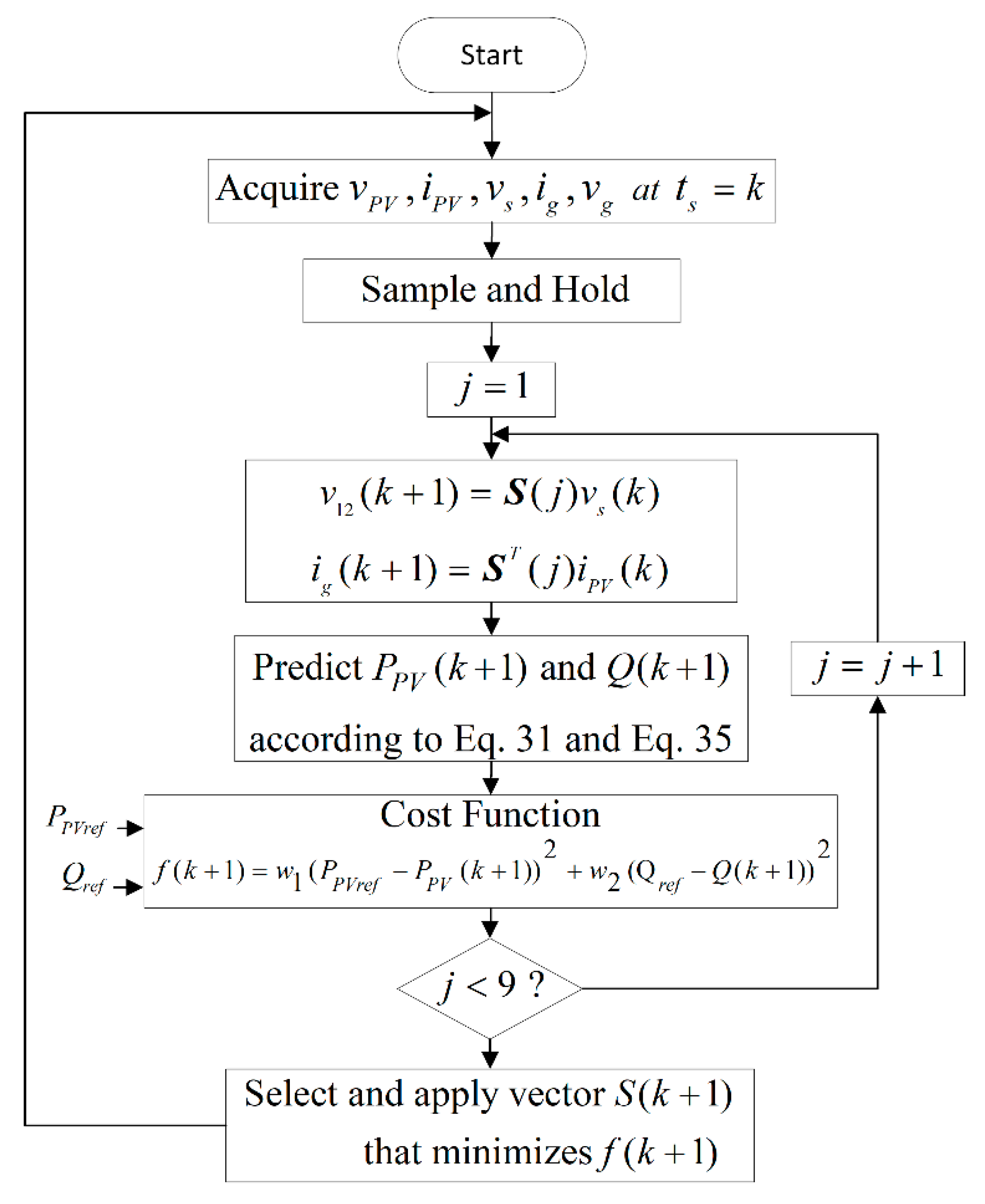
3.3. Cost Function and Selection of Swtiching Vector

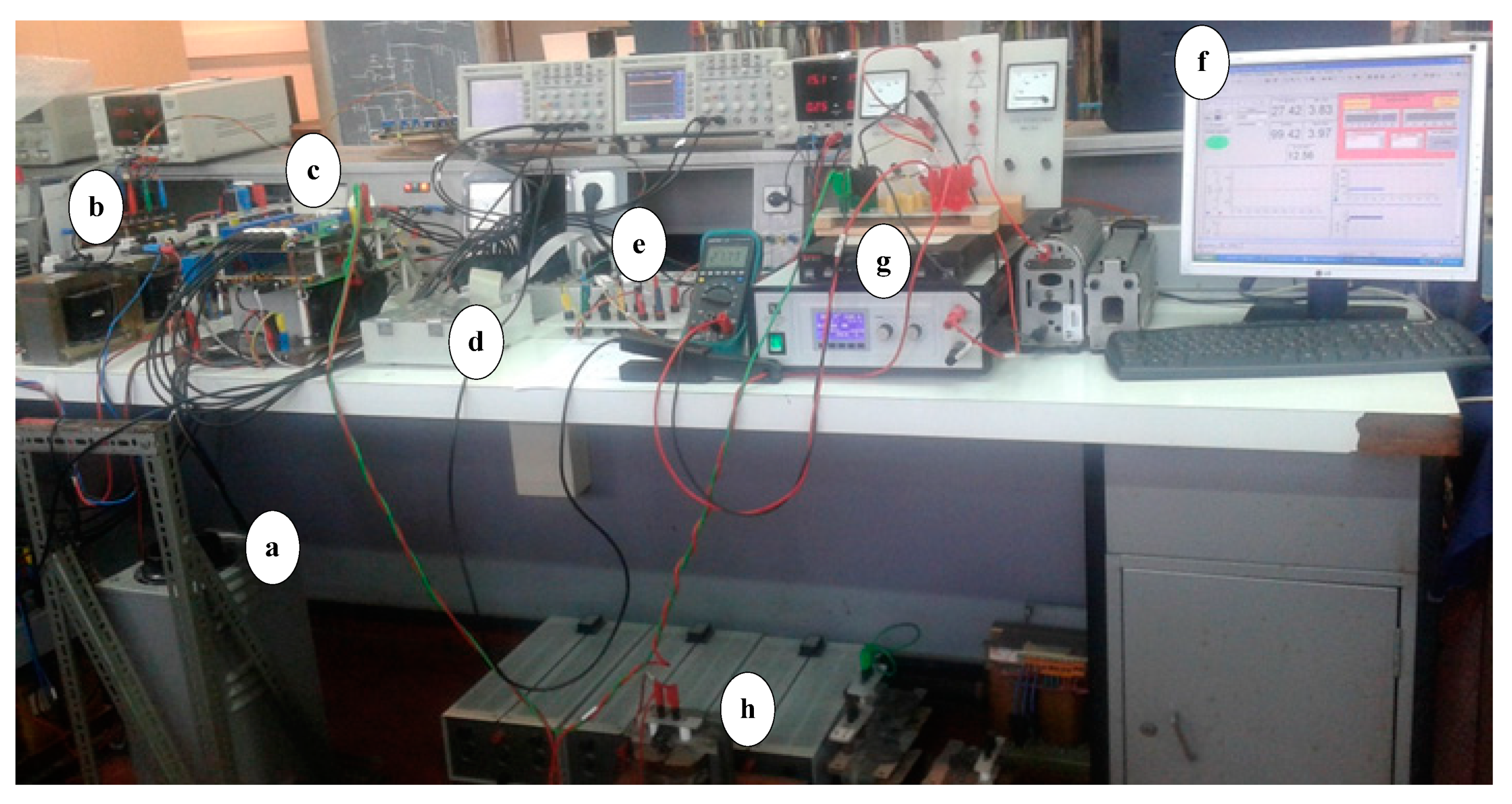
The selection of the optimal switching vector for the next sample is obtained by minimization of the cost function f(k + 1), that evaluates the error of the controlled variables. To ensure that the predicted active and reactive power reach the reference values, the cost function f(k + 1) is used to minimize the squared errors (Equation (36)), where $P_{PV,ref}$ and $Q_{ref}$ are considered as the set point references for the controller and w₁, w₂ are the weights for the active and reactive power, respectively.

$$f\left(k+1\right)=w_1{\left(P_{PV,ref}-P_{PV}\left(k+1\right)\right)}^2+w_2{\left(Q_{ref}-Q\left(k+1\right)\right)}^2$$

(36)

The procedure to select the optimal switching vectors is summarized in the flowchart of Figure 4.

The proposed controller structure used in the simulations and to obtain the experimental results is presented in Figure 5.

4. Results

In this section, a 600 W, three-phase grid-connected CSI based PV system is simulated in a MATLAB/Simulink environment, and experimental results are obtained using the laboratory setup shown in Figure 6.

The experimental prototype is implemented using a controlled DC power supply (1.5 kW, 360 V, 15 A) to emulate the behavior of PV panels. The rapid prototyping software and hardware DSPACE ds1103 and its Control Desk interface are used. A field-programmable gate array (FPGA) from Xilinx, model Virtex-6 FPGA ML605, is used to handle the timing requirements of the commutation process. The specification data of the experimental setup are listed in

Table 3. System specification data.

Item	Value
Grid frequency (Hz)	50
Grid phase voltage, rms value (V)	110
Grid filter inductance (mH)	4
Grid side filter damping resistance (Ω)	33
Grid filter capacitance delta (μF)	6
DC link inductance (mH)	12.5
Sampling time (μs)	20
PV Power (W)	600

.

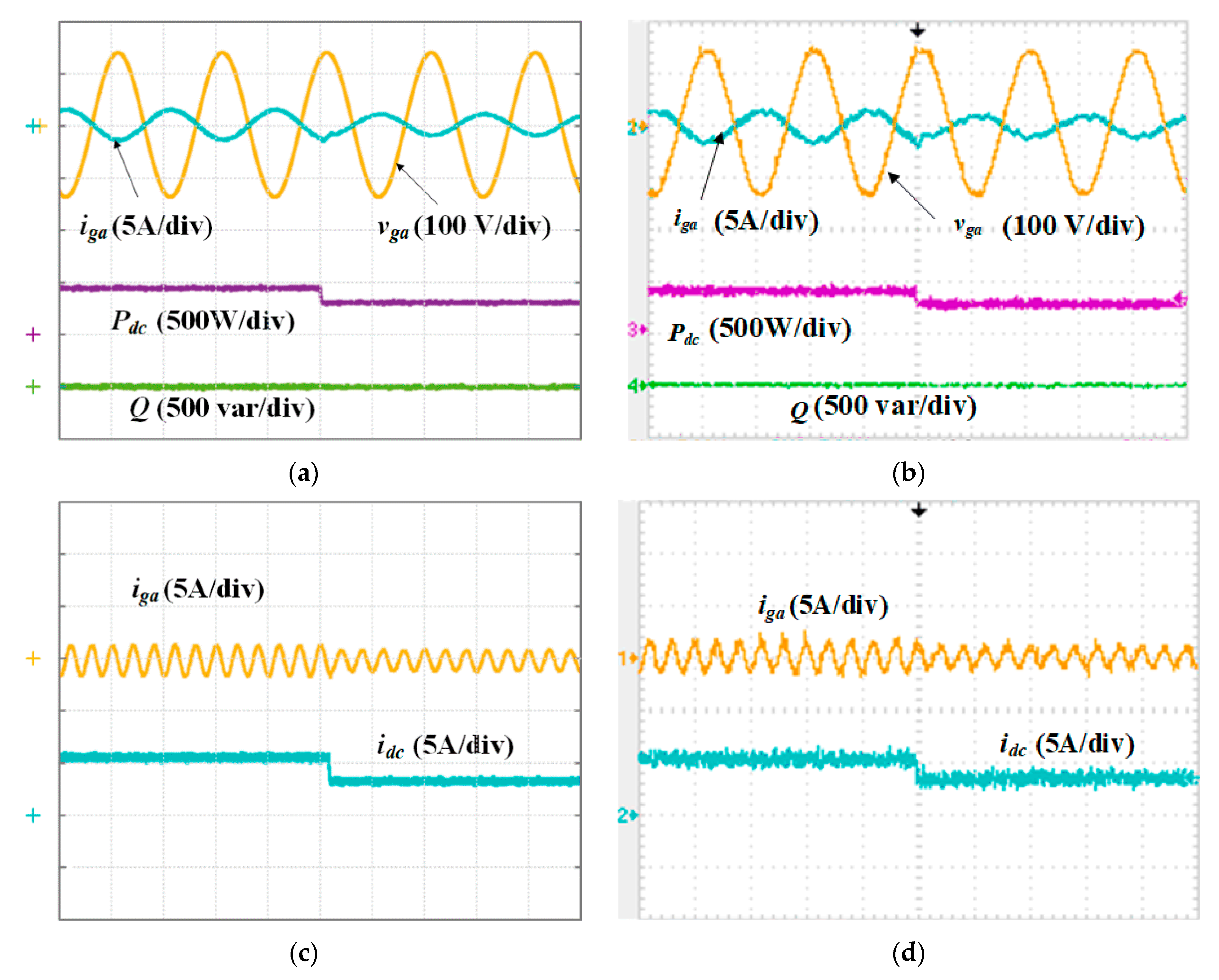
4.1. Response to a Step in Power

In this case, the proposed system is assessed for a PV power change from P_PV = 400 W to P_PV = 280 W at Q = 0 var. The main values used in the simulations and in the experiments are presented in

Table 4. Simulation data.

Grid Phase Voltage (V)	DC Voltage (V)	Pdc, ref (W)	Qref (var)
110	70	Step: 400 to 280	0

. The system is tested at 110 V phase grid voltage and around 70 V at the DC side (PV panel emulator).

Figure 7 depicts the simulation and experimental results for this case: Figure 7a,b shows one of the grid phase voltages v_gan and the corresponding grid current i_ga, the power measured in the DC side P_dc, and the reactive power Q in the connection to the grid. When the PV power is reduced from P_PV = 400 W to P_PV = 280 W, the AC current reduces from i_ga = 1.4 A to i_ga = 1.07 A. At the PV power change, the DC current i_dc reduces from i_dc = 6 A to i_dc = 4 A, as shown in Figure 7c,d.

The results show that the power on the DC side is controlled and tracks the step in the reference. The phase current is nearly sinusoidal and is out of phase with the grid voltage (assuming power flow from grid side to DC side). Also, the reactive power in the connection to the grid is nearly zero and not affected by the step in the active power.

The total harmonic distortion (THD) of the grid currents at maximum PV power (P_PV = 540 W) is presented in Figure 8, calculated using a fast Fourier tool analysis (FFT) in PowerGUI block. It can be seen that the measured value, obtained with a Fluke 1735 (compliant with IEC 61000-4-7 Class II), is 4.1%, thus less than the 5% set as the maximum by international standards.

Figure 9 depicts the simulation and experimental results obtained using the DPPC at DC voltage v_pv = 90 V and 110 V grid phase voltage, at maximum PV power (P_PV = 540 W). From Figure 9a,b, it can be seen that the current and voltage are out of phase, thus guaranteeing a nearly unitary power factor. The power supplied to the grid is slightly lower than 540 W and the reactive power is Q = 0 var.

These results show that the three-phase grid currents in Figure 9c,d are balanced and their ripple is low.

Comparing the simulation and the experimental results, it can be seen that they are very similar, proving the effectiveness of the proposed DPPC.

4.2. Active Power and Reactive Power Control Using DPPC

In this section, the proposed system is tested for two operating scenarios: one for a step change in the reactive power and the other for the tracking of a PV power profile.

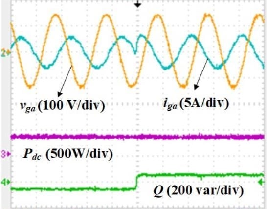
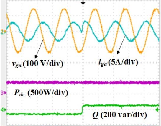
4.2.1. Step in the Reactive Power Q (Leading and Lagging)

This case study presents the PV system performance for a step change in the reactive power. The injection of reactive power in the PV system has many different strategies that are summarized in [4]. Here, the set point for the reactive power is used as a fixed value, and the limitation of reactive power depends on the maximum power capacity of the CSI. Figure 10 shows the dynamic response of the grid-connected PV system when changing from lagging to leading mode. Figure 10a shows one of the grid phase voltages v_gan and the current i_ga, in the same phase, for reactive power changing from Q = −40 var to Q = 40 var at P = 350 W operation. Figure 10b shows the three-phase grid currents i_gabc, (i_gmax = 2.6 A) and the current in the DC link, i_dc.

The results depicted in Figure 10 show a transition from leading to lagging power factor, where the DPPC controller provides a fast, yet smooth response, tracking the step in the reactive power reference. The active power remains unaffected, showing the effectiveness of the active and reactive power decoupled control.

When the reactive power changes, then the phase of the grid currents also changes. However, there are no disturbances or significant distortion in the current waveforms.

4.2.2. PV Power Profile Control

In this case, the daily PV power profile and the injection of reactive power are controlled using the DPPC. The reactive power is controlled to be at its maximum value during the day, at maximum PV power, and to be zero at night. The grid-connected PV system acts as a STATCOM (Static Synchronous Compensator), as shown in Figure 11a, where it can be seen the maximum reactive power injection Q = 100 var in the grid during the day at the peak PV power profile. The experimental conditions for this case study are listed in

Table 5. Experimental conditions for PV power profile control.

Grid Phase Voltage (V)	DC Voltage (V)	Pdc, ref (W)	Qref (var)
110	90	0 to 500	Step: 0 to 100

.

The results shown in Figure 11a indicate that the controller is able to track the maximum power. Also, the DPPC guarantees active and reactive power decoupling, as the step in the reactive power does not affect the active power.

Figure 11b,c present the grid phase voltage v_ga and the corresponding grid phase current i_ga for a step change in the reactive power Q, from Q = 0 var to Q = 100 var (Figure 11b), and then from Q = 100 var back to Q = 0 var (Figure 11c). The results obtained show that the grid current i_ga is leading the grid voltage v_ga at maximum Q and out of phase at Q = 0.

5. Conclusions

The objective of this paper was to provide contributions to the increasing trend in using CSIs in PV systems, which result in increased power density, lower costs, and increased lifetime of the inverter.

A state of the art for CSI control for PV applications was provided while emphasizing the advantages of single state topologies against two stage topologies.

The equations of the dynamics of the PV power and the AC reactive and active power were derived and provided the basis on which the DPPC was designed.

The synthesized DPPC directly tracks the power references based on the prediction of the PV power and on the AC active and reactive power. A quadratic error cost function was proposed with separable parameterizable weights for the PV power and the grid reactive power.

Simulations and experimental validation were obtained for steps in both the active and reactive power, showing the ability of the controller to track both references separately while maintaining values of THD within standards regulations.

The tracking performance was tested experimentally by submitting the controller to a typical power profile where the converter was able to track the maximum power along the profile while showing the ability to control the reactive power fully decoupled from the active power reference.

References

1. Wang, H.; Mancarella, P. Towards sustainable urban energy systems: High resolution modelling of electricity and heat demand profiles. In Proceedings of the 2016 IEEE International Conference on Power System Technology (POWERCON), Wollongong, NSW, Australia, 28 September–1 October 2016; pp. 1–6. [Google Scholar]
2. REN21. Connecting the Dots. Available online: http://www.ren21.net/ (accessed on 22 November 2018).
3. Kouro, S.; Leon, J.I.; Vinnikov, D.; Franquelo, L.G. Grid-Connected Photovoltaic Systems: An Overview of Recent Research and Emerging PV Converter Technology. IEEE Ind. Electron. Mag. 2015, 9, 47–61. [Google Scholar] [CrossRef]
4. Bae, Y.; Vu, T.; Kim, R. Implemental Control Strategy for Grid Stabilization of Grid-Connected PV System Based on German Grid Code in Symmetrical Low-to-Medium Voltage Network. IEEE Trans. Energy Convers. 2013, 28, 619–631. [Google Scholar] [CrossRef]
5. Momeneh, A.; Castilla, M.; Miret, J.; Martí, P.; Velasco, M. Comparative study of reactive power control methods for photovoltaic inverters in low-voltage grids. IET Renew. Power Gener. 2016, 10, 310–318. [Google Scholar] [CrossRef] [Green Version]
6. IEEE Standard 1547-2018. IEEE Standard for Interconnection and Interoperability of Distributed Energy Resources with Associated Electric Power Systems Interfaces; The Institute of Electrical and Electronics Engineers Standards Association: Piscataway, NJ, USA, 2018. [Google Scholar]
7. Standard IEC 61000-3-2:2018. Electromagnetic Compatibility (EMC)—Part 3-2: Limits—Limits for Harmonic Current Emissions (Equipment Input Current ≤16A per Phase); International Electrotechnical Comission: Geneva, Switzerland, 2018. [Google Scholar]
8. IEEE Standard 519-2014. IEEE Recommended Practice and Requirements for Harmonic Control in Electric Power Systems; IEEE Power and Energy Society; The Institute of Electrical and Electronics Engineers Standards Association: Piscataway, NJ, USA, 2014. [Google Scholar]
9. Standard IEC 61727. Photovoltaic (PV) Systems—Characteristics of the Utility Interface; International Electrotechnical Comission: Geneva, Switzerland, 2004. [Google Scholar]
10. Teodorescu, R.; Liserre, M.; Rodriguez, P. Grid Requirements for PV. In Grid Converters for Photovoltaic and Wind Power Systems; John Wiley and Sons Ltd.: Chichester, UK, 2011; pp. 32–42. [Google Scholar]
11. Al-Shetwi, A.Q.; Sujod, M.Z. Grid-connected photovoltaic power plants: A review of the recent integration requirements in modern grid codes. Int. J. Energy Res. 2018, 42, 1849–1865. [Google Scholar] [CrossRef]
12. Mirhosseini, M.; Pou, J.; Agelidis, V.G. Single- and two-stage inverter-based grid-connected photovoltaic power plants with ride-through capability under grid faults. IEEE Trans. Sustain. Energy 2015, 6, 1150–1159. [Google Scholar] [CrossRef]
13. Liang, X. Emerging Power Quality Challenges Due to Integration of Renewable Energy Sources. IEEE Trans. Ind. Appl. 2017, 53, 855–866. [Google Scholar] [CrossRef]
14. Meneses, D.; Blaabjerg, F.; García, Ó.; Cobos, J.A. Review and Comparison of Step-Up Transformerless Topologies for Photovoltaic AC-Module Application. IEEE Trans. Power Electron. 2013, 28, 2649–2663. [Google Scholar] [CrossRef] [Green Version]
15. Buticchi, G.; Barater, D.; Lorenzani, E.; Concari, C.; Franceschini, G. A Nine-Level Grid-Connected Converter Topology for Single-Phase Transformerless PV Systems. IEEE Trans. Ind. Electron. 2014, 61, 3951–3960. [Google Scholar] [CrossRef]
16. Shayestegan, M. Overview of grid-connected two-stage transformer-less inverter design. J. Mod. Power Syst. Clean Energy 2018, 6, 642–655. [Google Scholar] [CrossRef] [Green Version]
17. Wang, H.; Blaabjerg, F. Reliability of Capacitors for DC-Link Applications in Power Electronic Converters—An Overview. IEEE Trans. Ind. Appl. 2014, 50, 3569–3578. [Google Scholar] [CrossRef] [Green Version]
18. Bindra, A. Wide-Bandgap-Based Power Devices: Reshaping the power electronics landscape. IEEE Power Electron. Mag. 2015, 2, 42–47. [Google Scholar] [CrossRef]
19. Costa, P.; Silva, J.F.; Pinto, S. Experimental evaluation of SiC MOSFET and GaN HEMT losses in inverter operation. In Proceedings of the IECON 2019, 45th Annual Conference of IEEE Industrial Electronics Society, Lisbon, Portugal, 14–17 October 2019. [Google Scholar] [CrossRef]
20. Jain, S.; Agarwal, V. A Single-Stage Grid Connected Inverter Topology for Solar PV Systems with Maximum Power Point Tracking. IEEE Trans. Power Electron. 2007, 22, 1928–1940. [Google Scholar] [CrossRef] [Green Version]
21. Wu, L.; Zhao, Z.; Liu, J. A Single-Stage Three-Phase Grid-Connected Photovoltaic System with Modified MPPT Method and Reactive Power Compensation. IEEE Trans. Energy Convers. 2007, 22, 881–886. [Google Scholar] [CrossRef]
22. Wang, H.; Blaabjerg, F.; Simões, M.G.; Yang, Y. Power control flexibilities for grid-connected multi-functional photovoltaic inverters. IET Renew. Power Gener. 2016, 10, 504–513. [Google Scholar] [CrossRef] [Green Version]
23. Dash, P.P.; Kazerani, M. Dynamic modeling and performance analysis of a grid-connected current-source inverter-based photovoltaic system. IEEE Trans. Sustain. Energy 2011, 2, 443–450. [Google Scholar] [CrossRef]
24. Klumpner, C. A new single-stage current source inverter for photovoltaic and fuel cell applications using reverse blocking IGBTs. In Proceedings of the IEEE Power Electronics Specialists Conference, Orlando, FL, USA, 17–21 June 2007; pp. 1683–1689. [Google Scholar] [CrossRef] [Green Version]
25. Umeda, H.; Yamada, Y.; Asanuma, K.; Kusama, F.; Kinoshita, Y.; Ueno, H.; Ishida, H.; Hatsuda, T.; Ueda, T. High power 3-phase to 3-phase matrix converter using dual-gate GaN bidirectional switches. In Proceedings of the 2018 IEEE Applied Power Electronics Conference and Exposition (APEC), San Antonio, TX, USA, 4–8 March 2018; pp. 894–897. [Google Scholar] [CrossRef]
26. Geury, T.; Pinto, S.; Gyselinck, J. Current source inverter-based photovoltaic system with enhanced active filtering functionalities. IET Power Electron. 2015, 8, 2483–2491. [Google Scholar] [CrossRef] [Green Version]
27. Geury, T.; Pinto, S.; Gyselinck, J. Assessment of Grid-Side Filters for Three-Phase Current-Source Inverter PV Systems. Int. Rev. Electr. Eng. 2016, 11, 567–578. [Google Scholar] [CrossRef] [Green Version]
28. Lorenzani, E.; Immovilli, F.; Migliazza, G.; Frigieri, M.; Bianchini, C.; Davoli, M. CSI7: A modified three-phase current-source inverter for modular photovoltaic applications. IEEE Trans. Ind. Electron. 2017, 64, 5449–5459. [Google Scholar] [CrossRef]
29. Kouro, S.; Cortes, P.; Vargas, R.; Ammann, U.; Rodriguez, J. Model predictive control—A simple and powerful method to control power converters. IEEE Trans. Ind. Electron. 2009, 56, 1826–1838. [Google Scholar] [CrossRef]
30. Rodriguez, J.; Kazmierkowski, M.; Espinoza, J.; Zanchetta, P.; Abu-Rub, H.; Young, H.; Rojas, C. State of the art of finite control set model predictive control in power electronics. IEEE Trans. Ind. Inform. 2013, 9, 1003–1016. [Google Scholar] [CrossRef]
31. Yaramasu, V.; Wu, B. Fundamentals of Model Predictive Control. In Model Predictive Control of Wind Energy Conversion Systems, 1st ed.; Wiley-IEEE Press: New York, NY, USA, 2016; pp. 128–130. [Google Scholar]
32. Rodriguez, J.; Cortes, P. Predictive Control of Power Converters and Electrical Drives, 1st ed.; Wiley-IEEE Press: New York, NY, USA, 2012. [Google Scholar]
33. Barra, K.; Rahem, D. Predictive direct power control for photovoltaic grid connected system: An approach based on multilevel converters. Energy Convers. Manag. 2014, 78, 825–834. [Google Scholar] [CrossRef]
34. Chaves, M.; Silva, J.F.; Pinto, S.F.; Margato, E.; Santana, J. A New Backward Euler Stabilized Optimum Controller for NPC Back-to-Back Five Level Converters. Energies 2017, 10, 735. [Google Scholar] [CrossRef]
35. Gambôa, P.; Silva, J.F.; Pinto, S.F.; Margato, E. Input–Output Linearization and PI controllers for AC–AC matrix converter based Dynamic Voltage Restorers with Flywheel Energy Storage: A comparison. Electr. Power Syst. Res. 2019, 169, 214–228. [Google Scholar] [CrossRef]
36. Feng, S.; Wei, C.; Lei, J. Reduction of Prediction Errors for Matrix Converter with Improved Model Predictive Control. Energies 2019, 12, 3029. [Google Scholar] [CrossRef] [Green Version]
37. Youssef, E.; Pinto, S.; Amin, A.; Samahy, A. Multi-Terminal Matrix Converters as Enablers for Compact Battery Management Systems. In Proceedings of the 45th Annual Conference of the IEEE Industrial Electronics Society, Lisbon, Portugal, 14–17 October 2019. [Google Scholar] [CrossRef]
38. Vazquez, S.; Rodriguez, J.; Rivera, M.; Franquelo, L.; Norambuena, M. Model predictive control for power converters and drives: Advances and trends. IEEE Trans. Ind. Electron. 2017, 64, 935–947. [Google Scholar] [CrossRef] [Green Version]
39. Masoum, M.; Dehbonei, H.; Fuchs, E. Theoretical and experimental analyses of photovoltaic systems with voltage and current-based maximum power point tracking. IEEE Trans. Energy Convers. 2002, 17, 514–522. [Google Scholar] [CrossRef] [Green Version]
40. Wheeler, P.; Zhang, H.; Grant, D. A theoretical and practical consideration of optimised input filter design for a low loss Matrix Converter. In Proceedings of the 5th International Conference on Power Electronics and Variable-Speed Drives, London, UK, 26–28 October 1994; pp. 363–367. [Google Scholar] [CrossRef]
41. Sahoo, A.; Basu, K.; Mohan, N. Systematic Input Filter Design of Matrix Converter by Analytical Estimation of RMS Current Ripple. IEEE Trans. Ind. Electron. 2015, 62, 132–143. [Google Scholar] [CrossRef]
42. Sudubhi, B.; Pradhan, R. A Comparative Study on Maximum Power Point Tracking Technique for Photovoltaic Power Systems. IEEE Trans. Sustain. Energy 2013, 4, 89–98. [Google Scholar] [CrossRef]
43. Pinto, S.; Silva, J. Sliding mode direct control of matrix converters. IET Elect. Power Appl. 2007, 1, 439–448. [Google Scholar] [CrossRef]
Figure 1. Representation of the single stage current source inverter (CSI) based three-phase grid-connected photovoltaic (PV) system.
Energies 13 03165 g001
Figure 2. Equivalent circuit of the PV cell.
Energies 13 03165 g002
Figure 3. P–I characteristic of PV array at different irradiance levels and at constant temperature 25 °C.
Energies 13 03165 g003
Figure 4. Flowchart of the direct power predictive controller (DPPC).
Energies 13 03165 g004
Figure 5. Proposed controller structure.
Energies 13 03165 g005
Figure 6. Experimental setup of the proposed system: (a) auto transformer; (b) grid side filter; (c) matrix converter; (d) field-programmable gate array (FPGA); (e) DSPACE hardware; (f) DSPACE control desk; (g) controlled DC power supply; and (h) DC inductance coil.
Energies 13 03165 g006
Figure 7. Simulation results (a,c) and experimental results (b,d) for a step change in PV power; (a,b) grid voltage vgan, (yellow), grid current iga, (blue), power Pdc in the DC side (pink), reactive power Q in the connection to the grid (green), for a time scale (10 ms/div); (c,d) grid current iga, (yellow), current in the DC link idc (blue), for a time scale (50 ms/div).
Energies 13 03165 g007
Figure 8. Total harmonic distortion (THD) of grid current igb.
Energies 13 03165 g008
Figure 9. Simulation results (a,c) and experimental results (b,d) for a constant PV power Pdc = 540 W; (a,b) grid voltage vga (yellow), grid current iga, power Pdc in the DC side (pink), reactive power Q in the connection to the grid (green); (c,d) grid currents iga, igb, igc.
Energies 13 03165 g009
Figure 10. Experimental results for a step in the reactive power. (a) Grid voltage vgan (yellow), grid current iga (blue), power Pdc in the DC side (pink); reactive power Q in the connection to the grid (green); (b) three-phase grid currents igabc, and current idc (green).
Energies 13 03165 g010
Figure 11. Experimental results for a daily PV power profile. (a) Power Pdc produced by the PV (blue) and reactive power Q (pink); (b) reactive power step from Q = 0 var to Q = 100 var; (c) reactive power step from Q = 100 var to Q = 0 var; (b,c) grid voltage vgan, (yellow), grid current iga, (green), reactive power Q (pink).
Energies 13 03165 g011