Article

Standard, Point of Use, and Extended Energy Return on Energy Invested (EROI) from Comprehensive Material Requirements of Present Global Wind, Solar, and Hydro Power Technologies

by
Carlos de Castro
1,2,* and
Iñigo Capellán-Pérez
1
1
Research Group on Energy, Economy and System Dynamics, Escuela de Ingenierías Industriales, University of Valladolid, Paseo del Cauce s/n, 47011 Valladolid, Spain
2
Department of Applied Physics, Escuela de Arquitectura, University of Valladolid, Av Salamanca, 18, 47014 Valladolid, Spain
*
Author to whom correspondence should be addressed.
Energies 2020, 13(12), 3036; https://doi.org/10.3390/en13123036
Submission received: 24 April 2020 / Revised: 4 June 2020 / Accepted: 6 June 2020 / Published: 12 June 2020
(This article belongs to the Special Issue Rethinking Energy: Earth System Science Approaches 2021)

Abstract

:
Whether renewable energy sources (RES) will provide sufficient energy surplus to entirely power complex modern societies is under discussion. We contribute to this debate by estimating the current global average energy return on energy invested (EROI) for the five RES technologies with the highest potential of electricity generation from the comprehensive and internally consistent estimations of their material requirements at three distinct energy system boundaries: standard farm-gate (EROIst), final at consumer point-of-use (EROIfinal), and extended (including indirect investments, EROIext). EROIst levels found fall within the respective literature ranges. Expanding the boundaries closer to the system level, we find that only large hydroelectricity would currently have a high EROIext ~ 6.5:1, while the rest of variable RES would be below 3:1: onshore wind (2.9:1), offshore wind (2.3:1), solar Photovoltaic (PV) (1.8:1), and solar Concentrated Solar Power (CSP) (<1:1). These results indicate that, very likely, the global average EROIext levels of variable RES are currently below those of fossil fuel-fired electricity. It remains unknown if technological improvements will be able to compensate for factors, which will become increasingly important as the variable RES scale-up. Hence, without dynamically accounting for the evolution of the EROI of the system, the viability of sustainable energy systems cannot be ensured, especially for modern societies pursuing continuous economic growth.

1. Introduction

The solution to the coupled problems of climate change, pollution, and the depletion of fossil fuels (FF) needs a rapid transition, in historical terms, from the current fossil-based energy system to one whose main energy sources will be renewable (renewable energy sources, RES). In the ongoing debate about the timing and the features of this transition, environmental, economic, political, and technological issues are pointed out [1,2]. With relation to the latter, the discussion has mainly addressed three interrelated aspects:
  • The requirements and future availability of minerals to build the infrastructures to harness, transform, transport, and store energy [3,4,5,6].
  • The maximum technological, economic and sustainable energy flows available (potentials) for each energy technology/resource [7,8,9,10,11,12].
  • The energy surplus generated by the different energy sources available to society for discretionary uses (from growing food to family support, as well as education, health, and cultural development [13]). The most popular indicator to measure the ratio of energy surplus with relation to the required energy investments is the energy return on energy invested (EROI), i.e., the ratio of the energy delivered and the energy consumed to deliver that energy in a given time, with very abundant literature focusing both at technology and system level at different geographical scales (see e.g., [3,14,15,16,17,18,19,20,21,22,23]).
Although much work has been carried out to estimate the EROI of individual RES technologies, important methodological discrepancies exist depending on the applied definition, the system design and location, the functional units, or the boundaries of the analysis (i.e., mine-mouth vs. final use or individual energy technology vs. energy system) [16,21,24,25,26,27,28,29,30,31]. Different methods have been developed in the literature [3,16,29,32,33]; however, the inter-comparison of the EROIs obtained by these diverse methods is far from being straightforward (and often even not possible in a consistent way). Hence, although the EROI is generally acknowledged as a relevant factor for robustly designing the energy transition, and many multidisciplinary studies and meta-analyses have been performed with the aim of synthetizing and standardizing the state-of-the-art of the field [14,19,20,25,34,35,36], this dispersion of methodologies, definitions, and results hinders the potential to use the EROI concept to adequately inform policy makers and society as a whole.
One of the open debates of greatest importance is whether the RES with higher potential have a sufficient EROI to maintain the energy “metabolism” of a large and complex civilization, such as the industrial-one. In fact, a favorable EROI over the long-term has been associated in fields such as biology or anthropology as a key driver of increasing complexity and evolution for plants, animals and humans [37,38,39,40]. However, the question on the minimum EROI for human societies remains arduous and elusive in the literature [13,38,41,42]. It has been indirectly approached in the literature through the comparison with FF under the logic that RES were found to have an EROI level at least as high as the one characterizing FF, then it could be assured that RES could also fuel complex modern societies.
On the one hand, those RES with a higher potential (i.e., wind, solar) have been generally found to have lower EROI standard (EROIst) than FF, especially when incorporating the energy costs of dealing with their variability [19]. However, some recent works have found that at the electricity generated level, the EROI of FF declines substantially, making that the EROI of RES could be, nowadays, in fact, better than the one generated by FF [16,33,43]. However, the comparison is not straightforward. Brockway et al. [16] use an input–output extended approach for estimating the yearly EROI of all aggregated FF at a global level without accounting for capital investments, which prevented the application of the same method for RES (hence, performing the comparison through literature review). Raugei [33] and Raugei and Leccisi [43] refer to some FF particular cases at a national level, taking, as a timeframe, the full lifetime of the power plants at the point of use level. It should also be taken into account that static EROI computations (over the lifetime) are not able to capture dynamic issues inherent to the dynamic nature of the energy transition, such as the requirement of up-front investments for the installation of new RES power plants [3] or the decreasing historical trend in the EROI of FF [16,19,44,45].
In this work, we contribute to this ongoing debate by estimating the current global EROI over the lifetime for the five RES energy technologies assessed to have the highest theoretical potential for electricity generation (solar Photovoltaic (PV) and Concentrated Solar Power (CSP), wind onshore, wind offshore and large hydroelectricity) [11,46]. We compute the EROI at standard or primary and point-of-use or final, and estimate the EROI at extended boundaries (full-system level). This approach allows us to identify those steps where more energy investments are required, as well as a consistent inter-comparison between the EROI levels of different technologies.
Two main novelties are applied with relation to the current state-of-the-art. First, an extensive and comprehensive literature review is performed in order to collate internally consistent data about the material requirements of each technology. In the cases where published data for an element/phase of the manufacture/installation of the technology was not found, the material requirements have conservatively been estimated from available data from other technologies (instead of being assumed 0 as most commonly performed in the literature). Second, we focus on performance parameters of real systems, globally, which contrasts with the widespread approach in the literature applying theoretical assumptions for modeling RES systems and/or focus on particular plants or countries (a method that frequently leads to “cherry picking”), which has been shown to overestimate the performance of real technologies and systems [25,47,48,49,50,51,52,53,54].
This work documents in detail the assumptions and data used to estimate the material and energy investments to install, operate, and maintain new RES infrastructures used in the MEDEAS modeling framework [3,55,56]. In this framework, the computation of the “static” (over the lifetime) EROI at three levels (standard, point of use, and extended) of the different energy technologies is an intermediate step to consistently integrate the mineral and energy requirements of RES in the wider modeling framework, able to represent the dynamic nature of the energy transition, as shown in a previous analysis on dynamic EROI based at the standard level [3]. This work reports updated and original results based on a more detailed lifecycle analysis, which have still not integrated in the MEDEAS models.
Section 2 overviews and compares the different definitions of EROI in the literature and Section 3 covers the methodology applied to estimate the EROI levels in this work. Results are presented and discussed in Section 4 and Section 5, respectively, and Section 6 concludes.

2. Overview of EROI Definitions and Their Implications for Society

A diversity of different methods to estimate the EROI of a given technology, energy resource, or full energy system exists in the literature, according to different criteria to select the system boundaries and interpret which is the energy “usable” by the society, different definitions, etc. [3,16,29,32,33].
In this work, we estimate the EROI at the three boundaries most common in the literature: the EROI standard or primary (EROIst, Equation (1)), EROI at the point of use or final (EROIfinal, Equation (2)) and EROI extended (EROIext, Equation (3)). The EROIst includes the on-site and offsite (i.e., energy needed to manufacture the devices and systems used later on site) energy requirements to get the energy (e.g., build, operate, and maintain a power plant). As the energy investments are usually computed in “primary” energy terms and the energy delivered is computed in final terms, a “quality” correction factor (g) is typically used to compare different technologies and sources [Note that the authors have elsewhere (cf. [3]) defined a different EROIst (between the classical EROIst used here and the EROIfinal) applied to the system level, including the energy investments associated to the management of renewable energy sources (RES) variability, as well as considering that the real useful energy for the society is the one reaching the consumers rather than the one delivered at the mouth-gate of the power plants]. The EROIfinal includes the energy costs to get and deliver the energy carrier to the point of use of society (e.g., refining, transportation, etc.). The EROIext includes the energy required to get and deliver a unit of energy (EnUdirect), as well as the indirect energy (EnUindirect, or supply chain energy investment in input-output (IO) terminology) required to produce the machinery and devices used to build, operate, and maintain a power plant or a transportation facility (tank truck, pipeline, etc.), as well as the energy required for exploration, investment, communication, labor, etc. Hence, the EROIext is the most significant EROI type, given that the discretionary uses of energy are the relevant ones at societal level.
EROIst = Energy   delivered   by   the   plant   or   energy   source   Energy   used   to   deliver   the   energy   by   the   energy   system = Efinal , out EnUprimary g
EROIfinal = Final   energy   delivered   to   the   final   consumer Direct   final   energy   used   to   deliver   the   energy = Efinal , out EnUdirect
EROIext = Final   energy   delivered   to   the   final   consumer Direct   +   indirect   final   energy   used   to   deliver   the   energy = Efinal , out EnUdirect + EnUindirect
Figure 1 shows graphically the three aforementioned definitions of EROI (standard, point-of-use or final and extended) based on a flow chart.
Figure 2 shows the implications for an energy system that maintains the same discretionary energy flow when the EROIfinal decreases from 9:1 to 3:1, even with less relative losses (greater factor {1}/{0}). To achieve the same level of discretionary uses of energy with a lower EROI of the system, the economic sectors related to energy production and the primary energy sources to be extracted and processed increase substantially (final energy processed by society increases 2.33 times in the example depicted in Figure 2).
Few works have, to date, dealt with the intricate issue of the minimum EROI to sustain modern complex societies. Different works, applying different methodologies [13,41,42], have suggested that a minimum EROIst of the system > 10–15:1 is required to sustain advanced industrial societies. However, these estimations are approximates being subject to important limitations, such as the reliance on prices of energies and, in some cases, are just educated guesses without calculations backing them. Hall et al. [38] went a step forward, finding that a minimum of EROIst = 3:1 for oil and liquid biofuels is required to reach the final consumer in the USA. Other studies, such as Brandt [57], have approached the topic from a more theoretical point of view. Moreover, these estimates do not reach the EROIext, which is the relevant boundary at system level. In fact, although an energy technology with EROIext >1:1 is a net source of energy for the society, a complex modern society with an EROIext very close to 1:1 would still not be viable due to at least four reasons:
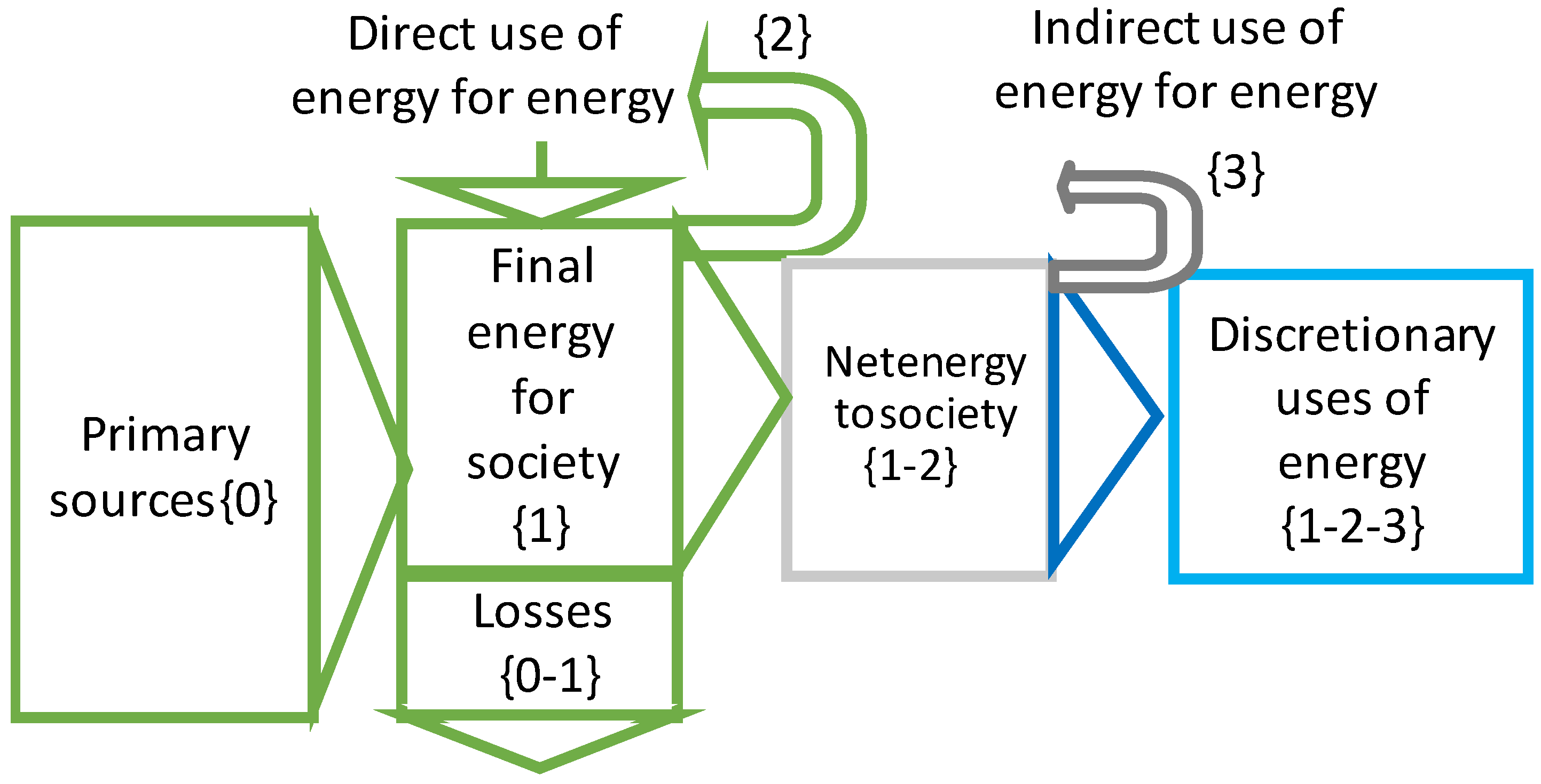
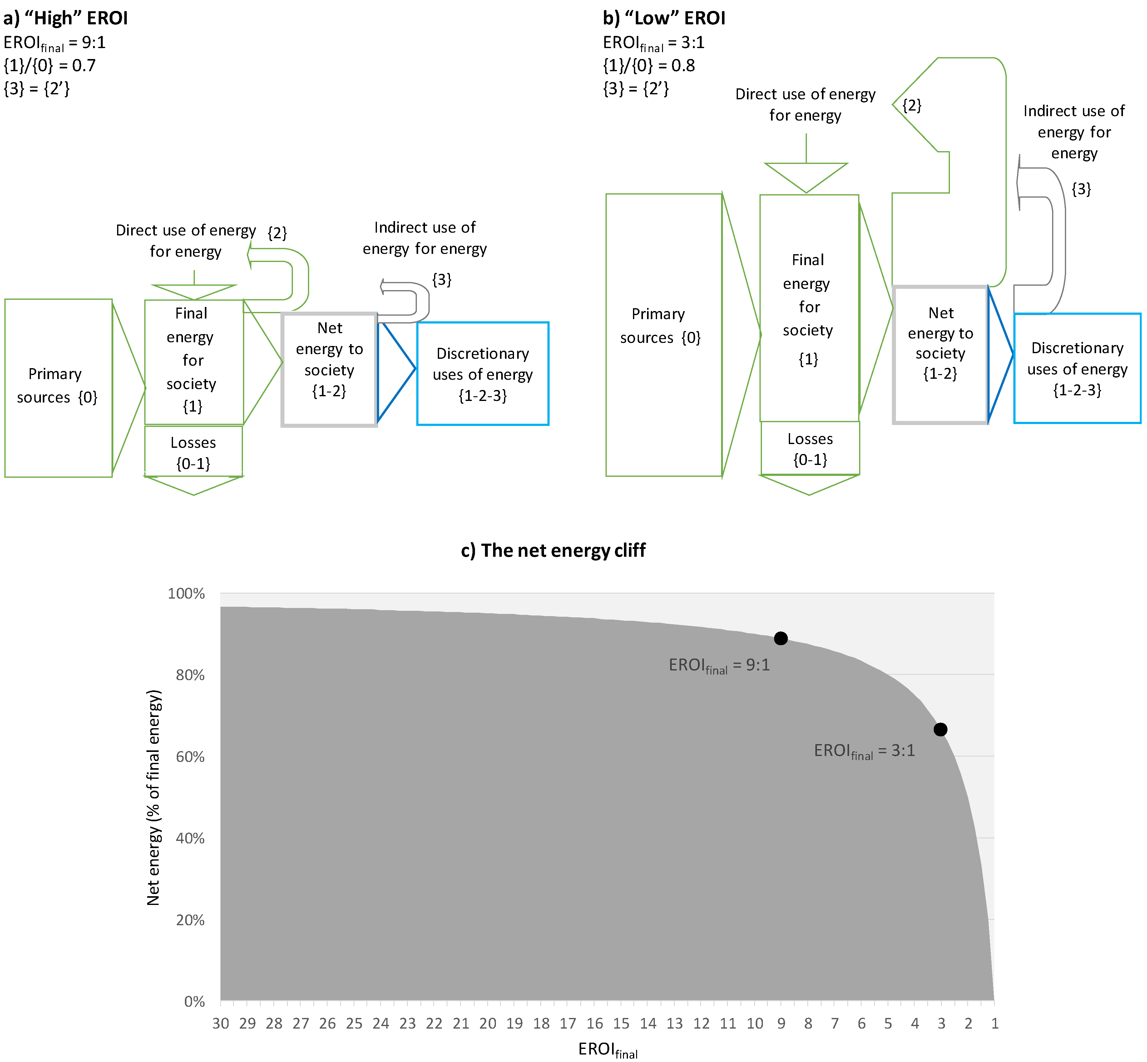
  • A low EROIext means that the energy metabolism ({0}, {1}, {2}, and {3}) represents a substantial part of the economy. Since each energy flux requires capital and workers, in that case the society allocates most parts of its capital and workers to the energy system, and not the discretionary uses. Therefore, a much lower diversity of jobs and enterprises can be attained in these conditions and the result is a much simpler society (as e.g., in pre-industrial times with most workers in the primary sector and very few in the tertiary sectors). In fact, there is an “EROI minimum”, below which a complex society tends to disappear or evolve towards simpler organizational forms [38,39,58]. In fact, when the EROI approaches 1:1, the capacity installed (and, hence, the primary energy required) tends to infinity if the same level of net energy is to be maintained (see Equations (9)–(11) in Capellán-Pérez et al. [59]).
  • The environmental impact depends on factors, such as the type of the energy resource (e.g., pollution and climate change caused by FFs’ combustion) and the size of the energy system (e.g., mining impacts, material residues, land-use, co-optation of fluxes of the biosphere—wind, biomass, etc.). Hence, for the same discretionary uses of energy, a lower EROI means larger environmental impacts and the need to divert a larger share of the final energy from discretionary uses to “defensive” costs [60].
  • Societies require a “security buffer” (i.e., buy “insurance”), to be able to overcome unexpected events, such as accidents or natural disasters (e.g., earthquakes).
  • Human inequality makes the metabolic system less efficient (in the real world, part of the discretionary energy uses will always be metabolically “useless”, such as luxuries of rich or corrupted people), so again, the supply of “useful” discretionary uses (food, domestic, education, etc.) requires an EROIext >1.
  • There is a critical additional reason in the context of the energy transition given that it will require the temporary fast growth of RES sources and the dismantling of the FF they replace. In this situation, the EROI of the full system will temporarily be well below the weighted average of the static EROI of the technologies and their supporting systems (e.g., grids, storage, etc.), as shown in [3]. Noteworthy, in a society where population and energy per capita are growing, this phenomenon of “energy trap” will be aggravated.
It has also to be highlighted that a minimum EROI to maintain a sustainable modern complex society cannot be established, precisely given that the reduced availability of discretionary energy as intermediary operations become less efficient is a gradual non-linear process with increasing and cascade consequences over time. Hence, it can also be useful to think about ranges and increasing levels of risk (see, e.g., discussions in Brandt [57] and around Figure 9 in [3]). This minimum EROI depend also ultimately on social decisions, depending on how each society decides to allocate the available resources in case of decreasing EROI between investments and consumption taking into account also social inequalities. See the Discussion section in this paper for our views on how to approach this issue in further research.

3. Methodology

This section documents the estimation of the current global EROI over the lifetime at three distinct boundaries (standard or primary, point-of-use or final and extended) for the five RES energy technologies assessed to have the higher theoretical potential for electricity generation (solar PV and CSP, wind onshore, wind offshore, and large hydroelectricity).
This section starts with the selection of the representative technologies (Section 3.1), follows with the definitions of EROI used at different boundaries (Section 3.2) and the material requirements to build, operate, and dismantle each RES technology power plant (Section 3.3). The details for the estimation of the EROI of each RES technology studied are collated in Appendix A and Appendix B.

3.1. Selection of Representative Technologies

In general, a “representative” technology is selected for each alternative technology on the basis of their current and the near future expected performance. Table 1 shows the selected representative technologies as well as the main references considered in this work for their material intensities. For the case of solar PV, a weighted average is computed for some minerals taking into account the current share of PV sub-technologies. Supplementary Material collates the material intensity for each technology and gives references and detailed comments. Current global average mineral recycling rates correspond to the share of recycled content (RC) in the fabricated metal from [61] (see Supplementary Material). Material losses in the gate-to-gate phase are conservatively estimated (see also Appendix C about conservative assumptions) (being recycled for other uses or not).

3.2. EROI Computation as a Function of the System Boundaries

3.2.1. EROI Expressions

Equations (4)–(6) show the gross standard, point-of-use or final and extended EROI expressions over the lifetime of the power system (plant or storage facility):
EROI st = E out , pp EnU direct st = = Capacity   power CF L ( 1 OL ) g st ( EnU New   cap + EnU O & M + EnU Decom + h j EnU Tra ) + SC
EROI final = E out , consumer EnU direct final = = Capacity   power CF L ( 1 OL ) ( 1 TDL ) g final ( EnU New   cap + EnU O & M + EnU Decom + EnU G & S + h j EnU Tra ) + SC ( 1 + TDL )
EROI ext = E out , consumer EnU direct final + EnU indirect
where:
Eout,pp: electricity produced by the power plant.
Eout,consumer: electricity delivered to the consumer.
Capacity power: nominal capacity power considered: 1 MW.
CF: capacity factor (dimensionless), the ratio of the actual electrical energy output over a given period of time to the maximum possible electrical energy output over the same period.
L: operational lifetime of the power system in seconds.
OL: operational electricity losses for each technology are estimated as a share of the electricity output of the power plant at the inverter or transformer meter, including local distribution grid losses to the transmission grid, operational shutdown losses, and expected degradation of the power plant. Double accounting with real CF is avoided by estimating the net future expected degradation, taking into consideration that most RES power plants are very young.
TDL: the transmission and distribution losses in the grid as a share of the electricity output of the power plant. They represent the losses from the transformer or inverter of the power plant to the final consumer. TDL = 0 for EROIst and TDL = 0.092 for EROIfinal and EROIext (based on the ratio of power plant net production of electricity at global level and the total electricity consumed in 2015. The electricity final consumption in 2015 was 1737 Mtoe and the net electricity production of the power plants was 1913 Mtoe (2091 Mtoe gross production—178 Mtoe self-consumption of electricity) [72]. Hence, TDL = 1 − 1737/1913 = 0.092. Final consumption to gross production losses were thus: 1 − 1737/2091 = 0.169; therefore, the electrical global mix in 2015 had OL = 1 − (1 − 0.169)/(1 − 0.092) = 0.085).
SC: electricity self-consumption of the facility from the grid for auxiliary devices (lights, pumps, motors, etc.). For EROIfinal, the TDL from the grid to the facility are considered equal to the TDL from the facility to the consumer (here, the consumer is the power plant).
EnUNew cap: Final Energy Used (Joules) for the construction phase of the new installed capacity (cradle to end gate). We further divide the EnUNew cap in three components (CtoG, GtoG and GtoE) to adapt to the data availability of material requirements in the construction phase (see Section 3.2.2 and Appendix A): EnU CtoG New   cap is the embodied energy in the Raw/resource to the Suppliers chain (cradle to gate in life-cycle analysis (LCA) terminology), EnU GtoG New   cap is the embodied energy from the suppliers to the finished products of the power plant or the Manufacturing phase (gate to gate phase), and EnU GtoE New   cap is the embodied energy in the Erection of the power plant.
EnUO&M: final energy used (Joules) in the operation and maintenance (O&M) of the installed capacity in their lifetime.
EnUDecom: final energy used (Joules) for decommissioning those infrastructures that have ended their lifetime. A 10% of the EnUNew cap is assumed for all technologies following [73] due to the lack of relevant global data. Other studies use a 50 to 100% of the site preparation energy costs (see Kis et al. [74]), which deliver similar results than the 10% of the EnUNew cap used here.
EnUG&S: final energy used (Joules) in grids, storage and other related infrastructures necessary to transport and manage the electricity to the point of use. For EROIst, EnUG&S = 0. For the sake of simplicity, we assign the O&M material costs of grids associated to the current mix as if they were independent of the technology (see Appendix B). However, due to the lower CF of variable RES relative to the current global mix and their variability, RES will likely require more new grids and other adaptation costs per MW as they scale up. Moreover, the storage per MW requirements (measured through their ESOI) are difficult to assign to a specific technology and have more sense in a dynamic transition scenario as done in [3].
EnUindirect: relative indirect EnU to direct EnU. We use 100%, i.e., EnUdirect = EnUindirect based on the comparison with meta-analysis that compare LCA versus Input–Output (IO) analysis for wind and solar (see Section 3.2.3).
EnUTra: final energy used for the transport of the materials: diesel and fuel oil (see Appendix B). Diesel and fuel oil are converted to primary energy with their respective factor hj estimated as the ratio between the well-to-wheels with the train-to-wheels (1.19 and 1.09 [75], respectively, see excel table in the supplementary material for references and details).
See next section for the method to assure consistency between primary energy inputs in the EnU computation and final energy outputs (g factor) for the three EROI indicators.
Figure 3 shows the conceptual representation of the energy inputs and output for power plants for variable renewable electricity generation and storage facilities, considering the different phases at different plant and system boundaries.

3.2.2. Computation of Direct EnUs from Material Requirements

The energy used by the energy system for the construction of new capacity (EnUNew cap), O&M activities (EnUO&M), grids and storage (EnUG&S) is estimated multiplying the material intensity for each category and technology by the energy consumption per unit of material consumption from open sources (MJ per kg, average between virgin and secondary materials considering current recycling rates). In the construction phase, EnU CtoG New   cap and EnU GtoE New   cap are computed taking as a basis the material requirements, while due to data scarcity referring to the Manufacturing phase EnU GtoG New   cap , we have assumed that this phase represents a fixed share for each technology of the Suppliers and Erection phases (see Section 3.3 and Supplementary Material for details and the rest of the phases). Data are cradle to the first gate (most data are from Hammond and Jones [76]); for the rest of the construction phase (first gate to final gate or manufacture phase), we take a constant share of the cradle to the first gate phase for each technology.
Figure 4 depicts the methodological process followed for computing the EnUs of the Construction phase (Cradle to Erection phase).
Material intensity data not available were conservatively estimated, e.g., assuming the same energy requirements per unit of material consumption for by-products than for the main mineral (e.g., Ga and Te). When no data on the energy consumption per unit of material consumption for recycled materials were found, it was assumed a value of 1/3 with relation to the virgin; this ratio was roughly estimated from available data for other minerals [76,77,78]. We review different items inter-comparing technologies to attain logical coherence (see details in Supplementary material).
As the basis of energy consumption is taken from literature that gives most data in “primary” terms and not in final terms, it is necessary to use a correction factor “g”.
Equation (7) represents the computation for each EnU (in final terms) for each energy technology i depending on the material intensity and energy consumption per unit of each material j consumption (in primary terms), weighted average taking into account current recycling rates (WECM(recycling rate)), at global system level.
EnU i = ( j Material   intensity ij [ kg MW ] WECM j ( recycling   rate j ) [ MJ kg ] ) g
The g factor is estimated at global system level, therefore, it is in reality an additional factor in the denominator of the EROI of Equations (4)–(6) using all EnUs as if all their energy consumption inputs were in primary terms. For EROIst, we take g = 0.47; that is the result at global level of the efficiency of current power plants (we estimate this value from International Energy Agency (IEA) Sankeys [72] at the plant phase). For EROIfinal and EROIext, we must take not only the plant phase but the overall energy system; therefore, g = {1}/{0} (see Figure 1) that at current world level is g = 0.688 (from IEA Sankeys [72] comparing total primary energy with final energy) (see also [25] for a discussion on this issue). Note that during the transition to RES this factor will be dynamic; in the case of electrification of the economy based on RES it will tend to 1; hence, reducing progressively its importance in the EROI computation [3].
When the literature splits between electricity and diesel consumption for some materials (these are the main but not the only carriers of final energy consumption) we simply add both in Joules as if they were in “primary” terms and correct to “quality” or final after the total EnU obtained. Of course, diesel energy is also not a primary energy although to our knowledge the literature does not apply to this item a correction factor, considering that is minor in comparison with electricity, therefore, the literature is slightly infra-evaluating here the EnU costs. The factor h applied to diesel could be translated to primary terms following the same logic than for power plants. The h factor for diesel for transport can be estimated comparing the “train to wheels” energy intensity of 35.9 MJ/l (the final energy carrier) with the “well to wheels” energy intensity of 42.7 MJ/L (the primary equivalent terms) [75]. In this case, the h factor would be 1.19. Then, as seen in the Equation (5), this again is multiplied by “g” to convert again from primary to a global final average energy. As g·h <1, here we are acknowledging a better quality of electricity versus diesel to perform work.

3.2.3. Estimation of indirect EnUs for EROIext

The indirect EnU, supply chain energy investment in input–output (IO) terminology, corresponds to the energy required to produce the machinery and devices used to build, operate and maintain a power plant, the associated transportation facilities (tank truck, pipeline, etc.), as well as the energy required for exploration, investment, communication, labor, etc. While process based methodologies allow computing the direct energy investments (and can capture some indirect costs), the computation of the indirect energy investments requires the application of a comprehensive method, such as IO, allowing to account for all the supply chain effects.
Song et al. [79] use a hybrid detailed analysis for fiber composites for automotive parts, finding that the direct process analysis use 50.3 MJ/kg; IO indirect costs add 61.5 MJ/kg, and Transportation + Packaging + Other processes (TPO) use 57.9 MJ/kg. Assuming that half of the TPO energy used can be related to the IO chain, then the EnUindirect would be even greater than the EnUdirect. Guan et al. [80] find similar results for the embodied energy costs of the building sector in China. When comparing process analysis LCA with Hybrid IO based analysis, they find that the gap is approximately 100%, therefore EnUindirect ≥ EnUdirect for this study case.
Even indirect rebound effects of the energy savings from the technological efficiency improvement are estimated greater than the direct ones when applying the IO methodology to capture both in the industrial sector of Taiwan [81] showing that the chain investments are important here and concluding that energy saving potential could be overestimated if not accounted for the indirect costs.
Similar conclusions can be extracted from the data of MEDEAS model at global level: the average indirect final energy demand in business as usual scenarios (BAU) scenarios (2020–2050) is roughly the same than the direct demand for all the final energy carriers, including the global electricity sector ([82] & Personal Communication (Jaime Nieto Vega, 19–11–2019)). Therefore, for the present and the foreseeable future in BAU scenarios, the EnUindirect is equal or greater than the EnUdirect at the system level.
The literature studying the indirect EnUs for RES is to date scarce. Two meta-analysis for wind and solar technologies have concluded that the EROIst based in process analysis tend to give a much higher EROI than IO analysis. Kubiszewski et al. [20] find an average of EROI of 24 from process analysis against 12 for the IO for wind farms. This result is consistent with a case study for wind in UK showing that IO-based hybrid LCA gives 2.33 times more gCO2e/kWh embodied emissions than a process analysis LCA and, therefore, indirect emissions (and very likely energy embodied) are greater than the direct ones [83]. The same seems to apply for PV, [30] reported ratios of 1.6–3.1 × times greater the result from IO with relation to process analysis LCA in the literature (see their Table 2). Provided that the numerator of the EROI is not different for process analysis or IO, the differences could be attributed mainly to the more comprehensive account of indirect costs with the IO methodology. Hence, in this work we assume that the indirect investments of RES represent at least 100% of the total direct energy investments estimated.

3.3. Material Requirements and Performance Factors Per Technology

A literature review was performed in order to identify the material intensity (kg/MW) of six key technologies for the transition towards fully RES based energy systems: solar PV, solar CSP, wind onshore, wind offshore, and large hydroelectricity. New installed capacity, O&M and dismantling activities are considered to estimate the material requirements.
We reviewed the requirements of a total of 58 materials, of which 19 minerals (aluminum, cadmium, chromium, copper, gallium, indium, iron/steel, lead, lithium, magnesium, manganese, molybdenum, nickel, silver, tellurium, tin, titanium, vanadium, and zinc) used at the power plants. Selection criteria was made on the basis of considering all relevant materials to accurately estimate the embodied energy for the EROI estimation, as well as potential critical materials identified in the literature (e.g., [6,84,85,86,87]), as well as on specific assessments (see [56]). A literature review was performed in order to collate the most comprehensible possible data from open sources about material requirements for each technology. This approach differs from published meta-analyses, which tend to focus on the average values of the range of parameters found in the literature [14,17,19,20,88]. In the cases where published data for an element/phase of the manufacture/installation of the technology was not found, the material requirements have conservatively been estimated from available data from other technologies (instead of being assumed 0 as most commonly performed in the literature). For example, since no data about the material requirements for fences for CSP power plants were found, the data estimated by Prieto and Hall [21] for fences for PV were used; similarly, since no data about land clearing for PV were found, so data for land clearing for CSP was applied instead [25,89], etc. No energy inputs are derived from monetary costs, and in the case of uncertainty about potential double accounting, material requirements are conservatively not included (see Appendix C). Besides material requirements, water requirements for solar PV and CSP are also estimated.
The next step is the computation of energy requirements associated to the manufacture and transport between the first gate (first transformation of raw materials) to the end gate (GtoG) before the erection of the power plant phase (the manufacture of complex devices and machines, e.g., the energy costs to produce a turbine from rods, laminates, etc.). This estimation is very difficult because the literature is very scarce comparing with the previous step (cradle to first gate). We have reviewed the available literature and for the sake of simplicity, and as a first conservative approximation, we have taken values corresponding to the lower bound of the literature range (see Appendix A and Appendix C). Dahmus and Gutowski [90] report, for simple machining, that this energy cost could be around 4–24% of the raw material phase (cradle to first gate) (for instance transform Al rod into a frame to assemble a PV panel). Boustani et al. and Ciceri et al. [91,92] report around 20–40% for more complex machines (such as refrigerators, air conditioners, or other machines of similar complexity), and even >100% for very complex devices like microchips, computers or the silicon wafer of a PV panel [92]. Inverters, turbines, motors, or computers are complex machines that at this gate-to-gate phase have a very likely measurable impact, but to the knowledge of the authors, very few studies are published that quantify it for power plants in an open methodology. Hence, we conservatively assume a machining energy cost of 15% of the total construction phase for hydro, wind, and CSP technologies due to the use of many simple machining process (like a mounted structure), but also with important complex ones (like wind turbines). For PV power plants, we use a lower estimation (10%) given that this phase, being very well studied for the silicon wafer, has already taken it into account in the cradle to gate phase.
Moreover, industrial production generates significant amounts of scrap: when an amount of material enters a manufacture factory, not all is incorporated to finished products. The scrap could be 10–60% of the embodied material in finished products. Moreover, most of the machining processes require some virgin or pure material because the recycled scrap cannot be fully reused [90]. As the materials used in the power plant are estimated at the plant, the percent (%) scrap in the manufacturing phase not entering the same manufacturing facility after recycling must be accounted in the cradle to gate phase. To avoid any possible double counting, we conservatively consider 10% as the lower end of Dahmus and Gutowski [90] to increase in this ratio the total amount of materials in the construction phase and hence their associated energy costs.
In relation to the electric grids, we estimate the materials required for the O&M of the currently existing grid (see Appendix B).
Finally, the energy for transport of the GtoE phase considering all the materials used in the facility and the O&M of the grid is computed (see Appendix B).
The Appendix B describes also the methodology used to estimate the EnUNew cap, EnUO&M and EnUG&S for each technology. EnUNew cap is estimated from material requirements for all technologies. The EnUO&M has been calculated for CSP, PV, and large hydro using data on reparation or substitution for 11 materials, while for wind technologies it has been estimated as a share of the construction phase based in the replacement of the average whole parts of the turbines during the lifetime of the farm.
See Supplementary material for the detailed results, comments, and references per material and technology.
Table 2 reports the performance factors (current global average) per technology used in this study.
Given that RES are characterized by strong increases of new capacity per year, and that this new capacity represents a non-negligible share of capacity with relation to the one already installed, we estimate the real CF for a year t (CF(t)) by assuming that only half of the capacity installed during that year (Δcap) generated electricity at full power that year (gen(t)) (Equation (8)):
CF ( t ) gen ( t ) cap ( t 1 ) + 1 2 Δ cap
The assumed lifetime of each technology is based in present global systems taking as reference the usual contracts of the operational life of the power plants and the system in our main literature studies for each technology. This lifetime is difficult to estimate because the average time in operation of the present power plants is very low due to the high recent growth of variable RES (we estimate: CSP = 7.2 years, PV = 3.8 years, Onshore Wind = 6.6 years, and Offshore Wind 4.4 years based in the capacity added in the history [93]). This parameter is hence subject to controversy (see for instance the discussion for PV from Ferroni et al. and the responses of Raugei et al. [26,31,100]). As the expected lifetime of these technologies is more than three times their current time in operation, it is difficult to estimate the average lifetime based in real numbers. The existence of failures—projects that do not reach the operational phase (or shut down after only a few years of operation) are usually not taken into account for the average lifetime (or the EnU costs incurred at system level)—prevents us from choosing the higher lifetime ranges collated in meta-analysis, because we are focused at global and historical real-data levels. For large hydro whose installed capacity grows at a much slower pace, we assume that the current average operational lifetime is half the lifetime considered. This is the reason why the power degradation assigned is only an estimation of the average power loss based in the % of dam failures in Table 2. For the rest, we take from Kis et al. [74] the annual degradation % of the power plants and estimate the already present power degradation based in the average operational time. The total expected power degradation in the lifetime minus the actual present degradation is the expected degradation in the pipeline that we use in Table 2.
For more methodological details for each technology, see Appendix B and Supplementary material.

4. Results

4.1. Current Global EROI of RES Technologies

Table 3 collates the obtained current global average standard, final, and extended EROI for the renewable electricity generation technologies studied in this work. We find EROIst levels of 28.4:1 (large hydro), 13.2:1 (wind onshore), 8.7:1 (wind onshore), 7.8 (PV), and 2.6:1 (CSP). Accounting for the transmission losses, the energy investments associated to the grids as well as the change from plant to full-system context implies a large gap between the three EROI boundary levels studied, a gap that other authors have also found for FFs (e.g., [16,33]). The energy investments associated to the O&M of the grids represent a relevant contribution, increasing around 9% (CSP), 19% (wind offshore), 30% (PV), and 40% (wind onshore) the embodied energy of the cradle to gate phase of each technology respectively (EnUNew cap + EnUO&M + EnUDecom + EnUTra following the notation of Equation (4)). In comparison, the refining and transport to final consumer of oil is typically < 15% [38]. We find EROIfinal levels of 13.0:1 (large hydro), 5.8:1 (wind onshore), 4.7:1 (wind onshore), 3.5:1 (PV), and 1.6:1 (CSP). The energy returns for each technology at the three boundary levels are large hydro > wind onshore > wind offshore > solar PV > CSP given that the same O&M for grids and indirect energy investments are assumed equally for all technologies. Finally, at extended level, large hydroelectricity continues to stand out, with high energy returns (6.5:1), followed by wind onshore (2.9:1), wind offshore (2.3:1), solar PV (1.8:1), and finally solar CSP (0.8:1). Hence, with an EROIext below 1:1, the CSP would in fact function rather as a storage device contributing to deal with short-term (hourly) variability (although at the cost of worsening the effects of seasonal variability [25]).
It should be acknowledged that the estimated global EROI current averages mask many regional differences depending on the quality of the resource. The next section takes the example of solar PV to illustrate how the EROI of the current electricity generation at the three boundaries estimated in this work may vary in different countries. We consider both big solar PV on land and rooftop given that we find that their EROI is ultimately quite similar, the lower requirement of material and energy inputs being compensated by a lower efficiency.

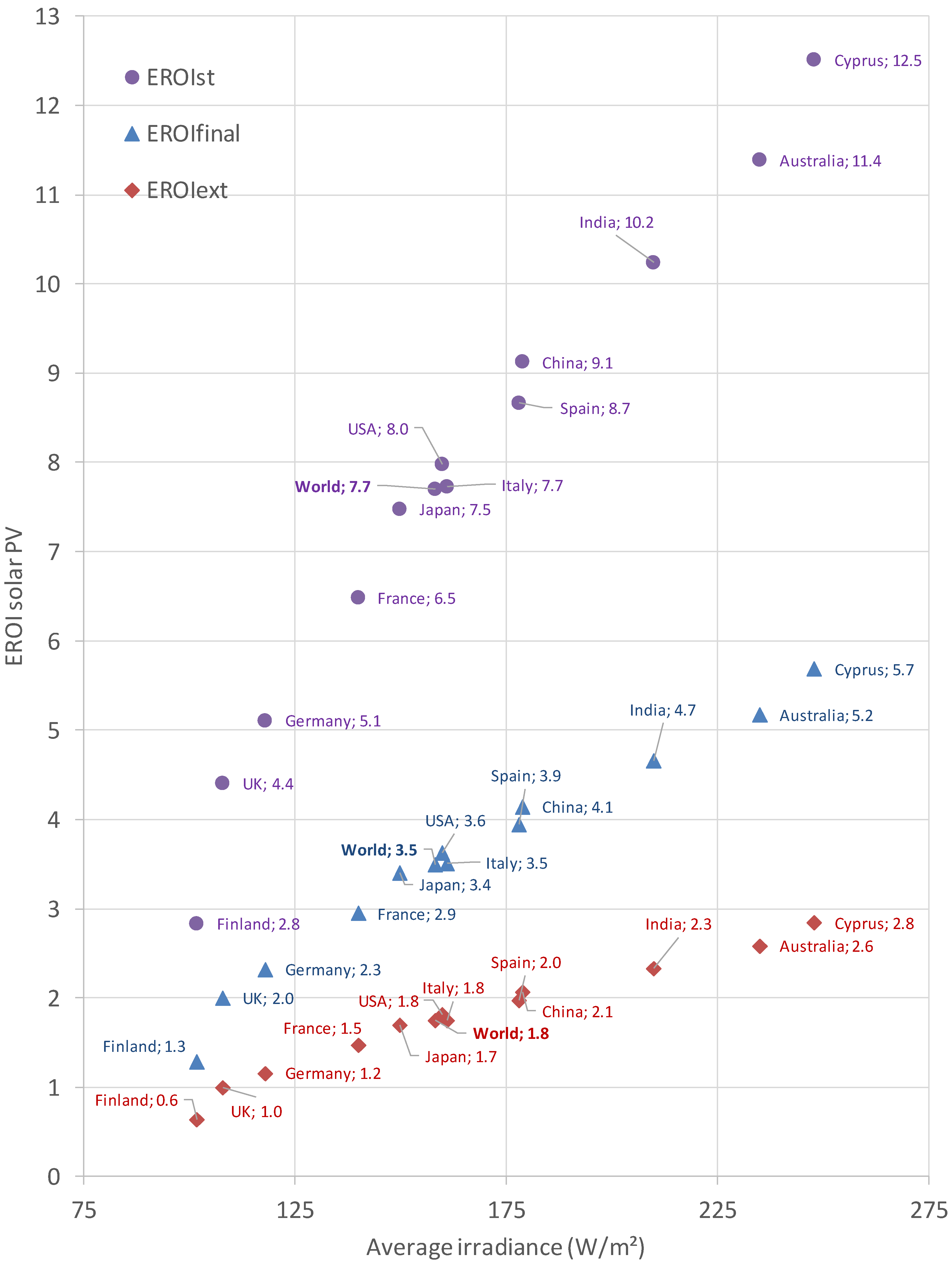
4.2. Geographically-Dependent EROI: Case Study for Solar PV

The RES availability and quality of their potentials inherently depend on geographical and climate characteristics (e.g., [10,101,102]), but also on the socioeconomic dimensions such as population density, which affects the density of required grids. However, to our knowledge, very few studies have attempted to date to estimate regional potentials of RES considering EROI levels [94,103]. Figure 5 shows an estimation of the different EROI levels of PV solar on land for a selection of countries at standard (EROIst), final (EROIfinal), and extended (EROIext) (gross) stages. This estimation is performed assuming that the global EROI is a weighted average of the installed capacity and the irradiance levels for the top-10 countries with more installed capacity at the end of 2016 [104]. These 10 countries together account for over 85% of the global installed capacity in that year. Two more countries are included to widen the scope of the analysis: Cyprus and Finland, which hold the maximum and minimum country-level average solar irradiances in the European Union [59]. We consider that the following factors vary for each country:
  • average solar irradiance per country estimated applying a Geographical Information System (GIS);
  • a reduction of the average performance ratio over the park’s life cycle due to higher temperature in the tropics;
  • a more efficient use of the space in countries closer to the equator, which reduces the energy investments in the phases of cement/concrete, iron/steel low, gravel/roads, and site works (which approximately correspond to 20% of the EnUNew cap of solar PV);
  • the same EROI for big solar on land and rooftop for each country (see Section 4.1).
As sources, we use data collected in previous work [59] combined with Martín-Chivelet [105] for the land occupation as a function of the latitude. Progressively broadening boundaries and considering geographical factors significantly affects the results: EROIst ranges 2.6–12.5.1:1, EROIfinal 1.3–5.7:1, and EROIext 0.6–2.8:1. Only in countries of great insolation, such as Cyprus or Australia, the EROIext levels would be close to the current onshore wind average of 2.9:1. In other countries, such as Finland or UK, we find an EROIext ≤ 1:1.The efficiency of the solar PV located at the global-average irradiance (168 W/m2) would then need to increase by ~50% in order to reach the current EROI of onshore wind, which is challenged by thermodynamic limits (e.g., [106]). It should be also highlighted that countries can enjoy the energy returns of power plants while avoiding the energy investments through international trade. In fact, it has already been shown that rich countries considerably benefit from international trade to net import energy (and carbon) intensive products from other countries, such as the BRIICS (Brazil, Russia, India, Indonesia, China) [107].

4.3. Comparison of the EROIst of RES Technologies with the Literature

As discussed in Section 2, the comparison of the EROI values obtained in the present study with other studies is tricky due to the methodological discrepancies existing in the literature and the uncertainty associated to the data collection (see Appendix C, Appendix D, and Appendix E for more details). Still, we report the comparison of our obtained results for EROIst with the literature range found in the review papers and meta-analyses to show how far or near we are of other published studies. We also compare with the EROIst calculations from Dupont and Kis et al., [74,94,103] since this team follows, to the knowledge of the authors, a methodology that is the closest to the one developed here; therefore, the direct comparison of results is the most meaningful. However, for a direct comparison a harmonization process should be endeavored with relation to the assumptions and performance factors (CF, g factor, etc.).
Table 4 shows that our EROIst results are within but on the lower bound of the literature for the RES technologies excepting for CSP [14,20,34,74,94,103,108,109]. Two main reasons explain this: (1) few studies use so many materials for the different construction, O&M, and dismantling phases, and (2) it is customary in the field to use favorable performance factors, which overestimate the average of real systems (see discussion in [25]). For CSP, our results are even below the low bound of the published ranges because, likely due to their relative low capacity installed, most studies rely excessively in theoretical grounds (as was demonstrated in [25]) and not in performance factors from real power plants. In any case, as argued in Section 2, we recall that the standard boundary for EROI is not sufficiently relevant to analyze the implications of the energy transition.

5. Discussion

We structure the Discussion section in two parts. First, a discussion on the potential role of future technological improvements to improve the EROI of the studied technologies in this study in the context of their likely large deployment in the next decades. Second, we give our views on how to properly take into account the effect of EROI for the energy transition and the potential implications we foresee.

5.1. On the Role of Future Technological Change

The EROIs computed in this study correspond to estimates for current RES technologies and power plants in operation. Future technological improvements may reduce the EnUs and/or improve the CF of the different RES technologies, as it has been happening in the last decades (e.g., increased cell efficiency and reduced wafer thickness in solar PV [31,110]). Since RES are expected to increase their share substantially in the next few decades, it is very relevant to assess to what extent future technological improvements and increase in mineral recycling rates may contribute to increase their current EROI levels. In fact, the recycling of materials generally requires less energy than their extraction from the mines (virgin), which holds true as long as the recycling rates do not approach 100% due to thermodynamic limits. Particularly, in the future there will be some very relevant factors, which will tend to offset potential technical improvements as the renewables progressively scale-up at large levels and gain a substantial share in the energy mix:
  • Additional energy investments and losses related with variability management of RES such as storage capacity (PHS, electric batteries, hydrogen, etc.), power-to-X, curtailment, and additional grids. The first three factors will tend to lower the EROI of the system due to the Energy Stored On energy Invested (ESOI) of the storage device, the increase of the transformation phases with associated transformation losses, and/or the diminishing effective CF of power plant being electricity curtailed. The fourth factor includes the substantial adaptation and expansion of the existing grids to cope with connecting the new RES power plants as well as helping to evacuate power when unevenly produced and demanded.
  • The effect of decreasing returns in the potential of renewables, i.e., after best places are occupied it is necessary to move to more uneconomical sites [94,103,111], phenomena that may be worsened in some cases by land availability constraints [59,112].
  • The increase in energy requirements for mineral processing related with ore grade decrease of minerals due to increased cumulated extraction [113,114,115].
  • Thermodynamic limits to the continuous reduction of required energy investments (e.g., related with limits to substitution).
  • Limits to recycling rates (other than thermodynamic): as aforementioned, most of the machining processes require some virgin or pure material because the recycled scrap cannot be fully reused [90].
  • The scarcity of some minerals in the future may drive the shift to more abundant minerals, which in turn are generally characterized by a lower performance (e.g., Ag instead of Al in mirrors, Nd in permanent magnets, Te in thin films, etc.) [63,86].
  • Thermodynamic limits from the side of generation. For example, the fact that there are absolute limits to the height of rotors for wind or the Benz law (modern large wind turbines already achieve peak performance coefficients in the range of 45–50%, which is pretty close to the limit of 59.26% [94])), or the limits in the conversion from sunlight to electricity, such as the Schokley–Queisser limit for single-junction solar cells. Although the latter limit could be overcome with multi-junction technologies, the key general question is how realistic it is, considering that the most sophisticated technologies—also related with the previous point—are really scalable at a significant level compared with total energy demand, or if, in the future, they will rather remain marginal.
Studies extrapolating the past evolution of EROI levels generally ignore all of the above factors and hence should be taken with care (e.g., [116]). Even studies that focus on past data are not totally reliable. For example, Louwen et al., [117], although they claim that all the PV systems analyzed include modules + inverter + mounting structure, in reality, the two more recent works (which seem to be largely driving their learning curve estimation, see their Figure 2b) correspond to (1) only PV modules, and (2) a solar rooftop system. Moreover, both of them use data from EU, not from China, where most production is located now.
Moreover, there is an additional issue related with the temporality of the transition, which will be especially relevant in the next few decades. Due to the fact that RES power plants, differently to FF ones, require large up-front costs and obtain delayed returns over the lifetime, a fast transition to RES would imply draining large shares of the energy available in order to sustain the energy transition. This means that, as shown in Capellán-Pérez et al. [3], which in fact is based on many of the assumptions and data reported here the EROI of the full system could temporarily be well below the weighted average of the static EROI of the technologies and their supporting systems (e.g., grids, storage, etc.). Hence, at system level, the fast penetration of renewables can lead to a situation of “energy trap”, i.e., a reduction in the discretionary energy arriving to society simultaneously with the increase in the consumption of primary energy [3,118]. Under this case, the efficiency of the full system measured as the primary to final energy ratio would worsen. Since some definitions, inputs and parameters are different in this work with relation to those used in Capellán-Pérez et al., [3] (here we perform a more detailed lifecycle analysis) in Appendix E we perform a harmonization of the results of both studies. The consistent comparison of the results obtained in both studies shows that the updated EROIst results presented in this work are lower (20–30%) for all the technologies, which reinforces the implications highlighted in the previous work [3] with relation to the potential scenario of “energy trap” during a fast energy transition. This phenomenon of “energy trap” would be aggravated in a context where population and energy consumption per capita are expected to continue increasing such as in the Green Growth paradigm.
Hence, the relevant feature is not the future EROI over the lifetime of each specific technology, but that of the full energy system in a dynamic, transitional way. Hence, the ultimate objective is to assess the potential implications that the dynamic EROI over time of the full energy system might imply for the thriving future societies (i.e., its implications for income, employment, etc., but also for dimensions more difficult to capture in quantitative modeling such as diversity in social functions). In this sense, it should be taken into account that a “sufficiently high” EROI is a necessary but not sufficient condition to achieve sustainable energy systems while maintaining high complexity in society. In particular, it does not give information about key aspects of the different energy technologies such as their environmental impacts (CO2 emissions, land occupation, etc.), social acceptance, future mineral availability, etc., as well as others such as cost effectiveness (although not totally being disconnected from energy effectiveness, cf. [119]). Although composite EROI indicators have been proposed to account for this (e.g., [60]), we believe that since sustainability is an inherent multi-dimensional concept its assessment has to be performed through a multi-dimensional set of indicators, being one of them the EROI.
It is noteworthy that most models used for advising policy (e.g., IEA, IPCC, national governments, etc.) neglect the energy investments related with the construction and operation of the RES power plants, as well as the implications on the full energy system [55,118,120]. Among the few models considering this factor are models published in the scientific literature with, unfortunately, little (if any) political incidence, such as GEMBA [121]; NETSET [122]; EETRAP [118]). The relation of EROI to net energy is non-linear (i.e., the “net energy cliff”), and consequently its impact can potentially be misjudged. Given the metabolic implications of the variation of the EROI of the system, assuring the consistency between physical investments (energy and materials) and economic investments seems a key precondition to ensure the robustness and viability of alternative sustainability scenarios, such as the Green Growth [123,124,125,126,127,128] or Post-Growth [129] scenarios.
We would like to conclude this section with a comment on the meaning of technological improvements and the relationship between economic (monetary) and biophysical (energetic and material) costs. Monetary cost reductions are typically identified with technological advances. For example, since the end of 2009, wind turbines prices have fallen by 30–40%, and solar PV module by around 80% [130] (and nearly 100× between the 1950s and the mid-2000s, more than any other energy technology in that period [131]). The levelized cost of electricity of solar PV (utility scale) has been estimated to have fallen by more than 60% between 2010 and 2016 [130]. However, in reality these historic cost reductions cannot be solely attributed to a reduction in the material and energetic intensities of a technology (technological improvement), given that they have also been critically affected by one-time financial (e.g., low interest rates to finance RES capital-intensive investments) and economic factors (e.g., economies of scale when increasing production, outsourcing to countries with less strict labor, environmental legislation, etc.). Additionally, the price of raw materials is subject to multiple influences (institutional framework, oligopolistic market structure, etc.) [132,133,134], which makes erratic their long-term evolution. For example, for the case of solar PV, it has been found that the reduction in average production cost and price of solar panels has been driven by factors, such as the reduction in the price of polysilicon, the increasing market penetration of lower cost firms from China, the increasing size of the facilities, and increases in industry investment, besides technological improvement, mainly in the form of the reduction in the use of polysilicon, and improvement of panel efficiencies [110,131]. Hence, a direct relationship between monetary costs and energy costs, or technological improvement, does not exist, although of course they are not totally independent [27,119].
Despite the aforementioned empirical evidences, the most common method used to represent endogenous technical change in energy–economy and integrated assessment models that inform energy planning and policy analysis is based on the extrapolation of historical learning curves (also known as experience curves) [2,130,131,135], which are a log–linear equation derived from empirical observations relating the unit cost of a technology to its cumulative installed capacity or electricity generated. A simpler version known as Moore’s Law treats time as the independent variable. This model is sometimes complemented by relating unit cost to cumulative expenditures for research and development, but it is, in any case, built under the assumption of perpetual cost reductions linked to increased production assuming that growth increases the likelihood of fundamental technological advances, incremental learning by doing, economies of scale in manufacturing, and standardization. However, in the era of a “full world” and over-exploited and degraded biosphere (“the global economy is now so large that society can no longer safely pretend it operates within a limitless ecosystem“ [136]), these dynamics cannot anymore be taken as granted in the future, which represents a paradigmatic change with relation to the past decades. “Natural resource flows are now the scarce factor, and labor and capital stocks are now relatively abundant. This basic pattern of scarcity has been reversed by a century of growth” [136].

5.2. Implications of Taking into Account the EROI for the Transition to RES

The first intuitive answer about the implications of taking into account the EROI of the RES during the energy transition can be given by the “net energy cliff”. Figure 6 shows the current global average EROI of each RES technology for electricity generation at the three boundaries studied in this study, represented as a share of the resulting share of net power vs. gross power in the net energy cliff. It can be seen that below levels of EROI < ~5–3:1, the share of net energy declines abruptly.
As aforementioned in the introduction, one of the open debates of greatest importance today in the context of the energy transition is whether the RES with higher potential have a sufficient EROI to maintain the energy “metabolism” of a large and complex civilization such as the industrial one. Given that, the estimation of a minimum EROI to maintain complex societies is a complex, and to date, elusive task involving both technical and societal issues, a large part of the literature has focused on the comparison with the EROI of FF as an indirect way of shedding light on this. In fact, in the case that RES were to be found to have an EROI level, at least as high as the one characterizing FF, then it could be assured that RES could also fuel complex modern societies.
However, the comparison of the EROI of RES at the extended boundary with the one of FF is far from being straightforward. To the knowledge of the authors, Brockway et al., [16] is the only study having computed the global average EROIext of FF at the electricity generation level. However, their input–output extended method is unsuitable for computing the EROI of RES given that it does not account for the energy associated to the capital investments (neither new capacities, decommission, nor new transmission lines required to move from EROI standard to point-of-use level). Although capital investments may represent a reduced part of the energy requirements for the case of an already extensively deployed industry, where most of the energy inputs are required in the O&M phase (as it can be assumed, not being so far from the situation of the current FF industry globally), for RES, the situation is exactly the opposite. Most energy investments are made upfront and the installed capacity is growing globally very fast. Although perfect comparability between both studies is not possible, we have made an effort to approximate the EROIext (gross) computed by Brockway et al., [16] for the aggregated FF to be roughly comparable with our method. When roughly accounting for the most relevant factors not considered in their study, we obtain a value of 3.9:1 (see Appendix D), which allows to conclude that their reported result of ~4:1 (gross EROIext) seems robust. Hence, it can be concluded that, very likely, the global average EROIext of variable RES is currently lower than those of FF for electricity generation.
This means that the current substantial lower power density (MWh/m2) [59,137] and higher material intensity (kg/MWh) [4,5] of variable RES, with relation to FF, make that the initial energy investment of RES weights more than the energy savings, due to the very low O&M energy requirements phase with relation to FF, where the situation is rather the opposite. The case of hydropower can be regarded as an exception given its very long lifetime (3–4 times for variable RES) and that although its power density is rather low, most parts of the surface is occupied by water “naturally” contained by valleys and mountains, and the built infrastructure is just concentrated in the dam.
Hence, of those RES with a higher techno-sustainable potential, the Figure 6c shows that only large hydroelectricity has currently a high EROIext clearly above the current global-average FF for electricity generation. Given that the techno-sustainable potential of large hydro is limited to less than double the current installed capacity (e.g., [138]), the transition to RES to supply the expected (increasing) energy demands will require large shares of the variable RES; hence, driving the EROI of the system to lower values, especially, as aforementioned, during the transition period before reaching a more stationary situation. Hence, to avoid driving the energy system to excessively low EROI levels, it is key that those uses that cannot be supplied by electricity, such as heat, are instead supplied directly by thermal technologies such as solar thermal, geothermal, and bioenergy in order to minimize energy conversions. Hence, there is a trade-off between the low EROI of RES for electricity with the strategy of managing variability through increasing the interconnectedness of the heat, cooling, transport, and electricity sectors [139] given that the latter introduces more conversions (i.e., losses) in the system. However, as previously highlighted, specific regional conditions are a key factor to take into account when designing the transition towards sustainable energy systems fully based on RES.
The above comparison holds for the current situation. However, it has to be taken into account that, in the future, there will be three concurrent dynamics that will affect the EROI of the system with different sign:
  • The EROI from FF globally is in a decreasing trend [16,19,44,45], a trend which will be intensified due to the higher share of unconventional fuels [19,140,141].
  • Technological improvement of RES (and in general any factor going in the direction of EROI max in the uncertainty analysis reported in Appendix C).
  • The likely large scale deployment of RES due to the enforcement of sustainability policies will (1) tend to replace FFs in the energy mix, and (2) drive an array of factors overviewed in the previous Section 5.1, which nowadays are negligible, but will become increasingly important as the renewables progressively scale-up at large levels and gain a substantial share in the energy mix. These factors will put a downward pressure on future EROI.
Future work will be directed to replicate the present study to compute the EROI of FF at the three EROI boundaries in order to be able to perform a consistent comparison. In any case, if globally the EROI from FF continues to fall, as it seems to have been doing in the recent past, there will be a point where FF will not be able to maintain complex industrial societies in the future, even if there are still resources in the Earth’s crust due to delivering insufficient energy surplus. This dynamic will be in reality aggravated by the fact that the environmental impacts produced by the burning of these FF (e.g., climate change impacts) will also contribute to hamper greatly our societies [1].

6. Conclusions

In this work, we have estimated the current global-average EROIst (standard farm-gate), EROIfinal (consumer point-of-use), and EROIext (extended, including indirect investments), for the five RES energy generation technologies assessed to have the highest techno-sustainable potential for electricity generation (solar PV and CSP, wind onshore, wind offshore, and large hydroelectricity). The same methodology, based on an extensive and comprehensive literature review, is applied in order to collate data about the material requirements for the power plants’ construction and operation of each technology, which allows for an internally consistent inter-comparison between the EROI levels of different technologies.
The obtained current global average EROI for each technology of electricity generation at the three boundary levels (standard, final, and extended, respectively) are large hydro (28.4, 13, 6.5:1) > wind onshore (13.2, 5.8, 2.9:1) > wind offshore (8.7, 4.7, 2.3:1) > solar PV (7.7, 3.5, 1.7:1) > CSP (2.6, 1.6, 0.8:1). Hence, accounting for the transmission losses, the energy investments associated to the grids as well as the change from plant to full-system context implies a large gap between the three EROI boundary levels studied, a gap that other authors have also found for FFs (e.g., [16,33]).
The extended boundary encompassing the implications for the full-system is the relevant perspective to assess the contribution in terms of energy surplus for discretionary uses to the society (e.g., growing food, family support, education, health, culture, etc.) of an energy technology. An array of factors make that, to maintain a sustainable modern complex society, the EROIext of the energy generation technologies should be distinctly greater than 1:1: a sufficient diversity of jobs and enterprises [38,39,58], the need to minimize the environmental impacts [60], the need of a “security buffer” to overcome unexpected events, such as accidents or natural disasters, and last but not least, the fact that most current societies are very unequal and, thus, are diverting energy towards metabolically “useless” purposes, such as those caused by inequalities. However, few works have, to date, dealt with the intricate issue of the minimum EROI to sustain modern complex societies, and none has been conclusive to date at extended level. When comparing with FF, our results indicate that the global average EROIext of variable RES is currently lower than the one corresponding to the global-average FF for electricity generation (4:1, reported by Brockway et al. [16], which adjusted to our methodology for comparability, corresponds to roughly 3.9:1). Large hydroelectricity stands out with a high EROIext of ~6.5:1 due to its particular features, while CSP stands in the opposite side with an EROIext < 1:1 meaning that this technology currently works rather as a storage device than an energy generation one. However, the heterogeneity of the EROI of variable RES at the geographical level is also a relevant feature to take into account, as it has been showed for the case of solar PV.
Our analysis is a static analysis. However, the implications of the EROI of RES must be assessed dynamically. During the forthcoming transition to RES, different dynamics will be simultaneously in action: declining EROI trends from FF, technological improvement of RES, and progressive emergence of an array of factors that, nowadays, are negligible, but which will become increasingly important as the renewables progressively scale-up at large levels and gain a substantial share in the energy mix: RES variability management, decreasing returns in the potential of renewables [94,103,111], the increase in energy requirements for mineral processing related with ore grade decrease of minerals due to increased cumulated extraction [113,114,115], thermodynamic limits to the continuous reduction of required energy investments (e.g., related with limits to substitution), limits to recycling rates, the scarcity of some minerals in the future [63,86], and thermodynamic limits from the side of generation. Additionally, the temporary fast growth of RES sources and the dismantling of the ones they replace (FF) will temporally reduce the EROI of the full system well below the weighted average of the static EROI of the technologies and their supporting systems (e.g., grids, storage, etc.). A shown in previous work [3], a fast energy transition with a very rapid growth of variable RES can generate issues at system level (energy trap). The present work, including a more detailed life-chain analysis, results in lower current EROIst levels than the ones used in [3] as inputs for the dynamic energy transition analysis (see Appendix E), hence, reinforcing the conclusions presented there. Noteworthy, the latter phenomena will be aggravated in a society where population and energy per capita have to continue to grow. Hence, the design of viable sustainable energy systems must take into account the dynamic evolution of the EROI of the system, especially for modern societies pursuing continuous economic growth which otherwise may derive in unintended “energy-trap” scenarios.
This work documents in detail the assumptions and data used to estimate the energy and material investments to install, operate, and maintain the RES with higher potential in the MEDEAS modeling framework [3,55,56]. In this framework, the computation of the “static” (over the lifetime) EROI of the different energy technologies is an intermediate step to consistently integrate the mineral and energy requirements of the energy transition in a wider modeling framework able to represent the dynamic nature of the transition. Further work will focus on the estimation of the mineral and energy requirements for the rest of energy technologies, which will allow the comprehensive computation of the variation of the EROI of the full energy system in scenarios of energy transition. A step further will assure the consistency with the monetary investments, which will allow to ultimately capture the implications for macroeconomic and socioeconomic dimensions, such as the change in the economic structure or the available income to households. This approach may ultimately allow to approach the issue of the minimum EROI to sustain complex modern societies from an endogenous point of view, taking into account both technical options and societal decisions, which could restrain or boost the vicious circle dynamics of declining EROI.

Supplementary Materials

The following are available online at https://www.mdpi.com/1996-1073/13/12/3036/s1.

Author Contributions

Conceptualization, C.d.C.; methodology, C.d.C.; validation, I.C.-P.; formal analysis, C.d.C.; investigation, C.d.C. and I.C.-P.; resources, C.d.C. and I.C.-P.; data curation, C.d.C. and I.C.-P.; writing—original draft preparation, C.d.C.; writing—review and editing, I.C.-P.; visualization, I.C.-P. All authors have read and agreed to the published version of the manuscript.

Funding

This work has been partially developed under the MEDEAS and LOCOMOTION projects, funded by the European Union’s Horizon 2020 research and innovation programme under grant agreements no 691287 and 821105, respectively. The authors are thankful as well for the support of MODESLOW (Modeling and Simulation of scenarios towards a LOW-carbon transition: The Spanish case), a Spanish national research project funded under the Spanish National Research, Development and Innovation Program (Ministry of Economy and Competitiveness of Spain, ref. ECO2017-85110-R). Iñigo Capellán-Pérez also acknowledges financial support from a Juan de la Cierva Research Fellowship of the Ministry of Economy and Competitiveness of Spain (no. FJCI-2016–28833).

Acknowledgments

Authors thank the Group of Energy, Economy, and Dynamics Systems (GEEDS) of the University of Valladolid for indirectly contributing to this work during group discussions.

Conflicts of Interest

The authors declare no conflict of interest.

Appendix A. EnUs

The Supplementary Material excel spreadsheet collates the materials required for the construction and operation of the power plants of the different technologies per MW (kg/MW). For each material, the embodied energy is given in primary terms (MJ/kg) using current recycling rates (Equation (7) of the main text). For the calculation of the denominator of the EROI (Equations (4)–(6)), we distinguish four EnU components:
Total EnUdirect: EnUNew cap + EnUO&M + EnUDecom wear cap + EnUG&S
where:
EnUG&S is calculated after the information in Appendix B (see also the tab “Electric grids” in the Supplementary Material).
EnUDecom = 0.1·EnUNew cap
EnUO&M is estimated annually; for solar technologies the material requirements and energy intensities are in the “Solar PV & CSP” tab, for wind technologies the EnUO&M is assumed to be 1% and 1.25% for onshore and offshore relative to their EnUNew cap, respectively, as explained in the “Wind onshore & offshore” tab of the Supplementary Material.
Finally, EnUNew cap is divided in three components:
EnU New   cap = EnU CtoG New   cap + EnU GtoE New   cap + EnU GtoG New   cap
Cradle to first gate (CtoG) is the part of a complete cycle analysis between the mineral mines extraction to the basic industrial material like rods, plates, etc., used by the industry. Gate to gate (GtG) represents the manufacturing phase: the process between rods, plates, etc. and the final form of these materials in a power plant (e.g., computer, frame of a PV plate, rotor, etc.).
EnU CtoG New   cap is the embodied energy in the Raw/resource to the Suppliers chain (cradle to gate in LCA terminology), EnU GtoG New   cap is the embodied energy from the suppliers to the finished products of the power plant or the Manufacturing phase (gate to gate phase), and EnU GtoE New   cap is the embodied energy in the Erection of the power plant. Both, EnU CtoG New   cap and EnU GtoE New   cap are calculated applying the Equation (7) to the data collated in the Excel spreadsheet for each item.
As explained in the main text, there is not enough detailed data of the Manufacturing phase EnU GtoG New   cap for RES technologies, and we have assumed that this phase represents a fixed share for each technology of the Suppliers and Erection phases:
EnU GtoG New   cap = x ( EnU CtoG New   cap + EnU GtoE New   cap )
As stated in the main text, taking into consideration the machining energy and the % of scrap in the manufacturing phase, x has been approximated to 0.25 for solar CSP (more precisely the calculation would be [1−(1−0.15) × (1−0.10)] = 0.235) for wind onshore and wind offshore, to 0.20 for solar PV.
Cumulative Energy Demand (CED) is a term with origin in the life-cycle analysis (LCA) community, where it is defined including all the primary energy harvested in the lifetime. However, this definition needs corrections to calculate EROI or the Energy Payback time. To avoid confusion of the different “CEDs” being used in the literature, and given priority to the historical precedence to the CED defined by LCA community, we apply in this paper the term Energy Used (EnU) instead of Cumulative Energy Demand (CED) (the same criteria was applied in precedent works of the authors [3,25]).

Appendix B. Material Requirements and Performance Factors Per Technology Details

Solar CSP (CSP with Molten Salt Storage Without Backup)
Performance Factors:
De Castro and Capellán-Pérez [25] showed that the current CF of CSP globally is <0.25; we use CF = 0.252 based in IRENA [93] for the sake of using the same reference for the different studied technologies. We take 25 years of lifetime [25]. SC = 9.1% is the 2014–2018 annual average from [95,96,97,98,99] (Kis et al. [74] give 15% of “parasitic loads” for CSP plants with storage. Kis et al., [74] give 15% of “parasite loads” for CSP plants with salt storage and 7.2% for no storage plants. Ramorakane and Dinter [142] give approximately also 15% for the power plant Andasol 3. The parasitic load (PL) is the self-consumption from the power generated but not dispatched plus the imported power from the grid. This imported power is at least 50% because during night the PL is around 50% of the maximum during the day. Ramorakane and Dinter do not give results for other auxiliary facilities like domestic illumination etc. therefore, 50% is very conservative. We conclude that is >7.5%. The rest until reaching 15% is from diesel and natural gas consumption in the own plant and could be considered as operational losses.
Material Requirements:
The main reference for estimating the required materials for this technology is a recent previous study from the same authors [25], which has been completed in this work with data from PV for diesel, evacuation lines, gravel (e.g., roads, protection) etc., (see details in supplementary material). Given that the density of material requirements (kg/m2) of CSP is ~3–4 × comparing to PV, it is very likely that this approximation is, thus, conservative.
We assume mirrors coated with a silver reflective layer as currently used despite the potential scarcity of this mineral in the future [63,86]. If considering aluminum mirrors instead, the EnUNew cap would increase by ~8% [25] and the efficiency of the system (equivalent CF) would decrease by ~14% [143], which would lead to an EROI of ~80% the reported here (EROICSP(Al) = EROICSP(Ag) × 0.86/1.08).
An additional 1.5% share of EnUNew cap has been conservatively considered in the decommissioning phase to account for small devices (pumps, valves, etc.), which other authors have estimated at 2.5% of the EnUNew cap [25].
Solar PV (Mainly Fixed-Tilt Silicon PV)
Performance Factors:
From IRENA we estimate a CF = 0.142 [93]. We take a lifetime of 25 years (15 years for the inverter) [21]. SC = 1% of electricity delivered at the plant, annual 2014–2018 average from [95,96,97,98,99] (Kis et al. [74] also give 1%).
Material Requirements:
Material data have been extracted and adapted from Frischknecht et al. [64], Valero et al., [62] (lower estimates), and from Prieto and Hall [21], in the latter case excluding data indirectly estimated from economic parameters (which could eventually be considered in a calculation of EROIext). For the remaining of materials not available from these sources, a conservative estimation from CSP data (25%) has been carried out taking into account that the density of material requirements of PV is ¼-1/3 that of CSP and that the surface power density of both technologies is similar [63].
For the data of “site preparation” we have considered 1/3 in relation to CSP values’ given that the PV power plants can be installed in zones with a steeper slope (e.g., [10]).
For the data of “silicon wafer”, we consider the performance parameters from Latunussa et al., [144] for recent technologies of 200 µm (0.5 kg/m2 accounting for the density of silicon) that use also Frischknecht et al. [64], which translate to >3500 kg/MW. MEDEAS literature review [62] identifies the range 3653–9000 kg/MW. For other technologies such as a-Si and thin-films, the wafer requires less materials and is energetically less costly, however its efficiency decreases significantly, around half [62] and need more infrastructures related with the land occupation (more fences, more soil works, etc. per energy delivered). In the case of thin-films, material scarcity may appear (Cd, Te, Ga, In and Ge, see [62]). We use, therefore, 3500 kg/MW conservatively.
PV Rooftop:
A rough first approximation to the EROI of PV rooftop has been made taking as a starting point the estimation for big solar PV on land. On the one hand, given that using an existing roof simplifies the construction process, we assume no energy inputs related to the categories of cement/concrete, iron/steel low, gravel/roads, site works and evacuation lines (see Supplementary Material); as well as reduces the size of the internal wiring (e.g., reducing the Cu use for this item). On the other hand, the transport energy phase could be greater because panels and other devices must be transported in a much more dispersed way, using vans that have a much more energy intensity in MJ/tkm terms than trucks (the same apply to the O&M costs). Moreover, given that rooftop PV has to adapt to the existing roof and its potential constraints in terms of tilt, shades, urban microclimate etc. its efficiency is generally lower than big solar on land (a ~20% lower efficiency following [59]). For the sake of simplicity, we assume that other potential reductions of materials (e.g., Al) are compensated by an increase in others (e.g., inverters (Frischknecht et al. p. 19 [64]).
Wind Onshore (2 MW Turbines)
Performance Factors:
CF = 0.242 in 2015 based in IRENA [93]. Lifetime 20 years based in [66]. Availability losses (3%) are taken from Dupont et al., [94], which are due to maintenance shutdown of production. SC = 2.1% is the annual 2014–2018 average for onshore and offshore from [95,96,97,98,99]. (Kis et al., [74] consider 3.5%).
Material Requirements:
The main reference for the materials requirements of wind onshore is GAMESA [66] due to its detailed accounting of data, which has been completed with MEDEAS literature review [62] and other sources. Although wind onshore turbines of higher capacity than the one considered in the GAMESA study currently exist at commercial level, the average global current installed capacity is lower than 2 MW.
Material requirements of Cu, Ni, Dy, and Nd have been collated from MEDEAS literature review [62]. In the case of Dy and Nd, although they will be likely scarce in the future, their influence in the EnU is limited. However, from the full EROI perspective its utilization is worth of given that they increase the efficiency of the turbine. In the case of mineral scarcity, the EROI levels estimated here would thus be an overestimation. However, from a socio-environmental perspective, it would be better not to use them given the high impacts of their mining [145,146].
For the O&M, we have followed the replacements of the components of the turbines following [147,148] assuming finally that the annual O&M phase is around 1% of the construction phase (which, in fact, is similar to the final results obtained for CSP).
Wind Offshore (Mainly 3.6 MW Turbines of London Array)
Performance Factors:
CF of 0.409 in 2015 based in IRENA [93]. We use the same lifetime (20 years), SC (2.1%) and annual degradation than wind onshore, although self-consumption and annual degradation could be bigger because the more aggressiveness of their environmental conditions (but Kis et al., [74] takes an SC = 0.7% that we consider of difficult explanation comparing with the 3.5% that they report for onshore).
Material Requirements:
The main reference for the material requirements of the wind offshore is [68], which computes data for mainly 3.6 MW turbines. This source is complemented with Smart Wind [69] project data and with wind (conservative) onshore specifications when specific data for wind offshore are not available.
London Array is one of the largest offshore wind plants in the world, and it is considered as a paradigmatic example of this technology. Data from this farm [68] have been contrasted with data from the Hornsea Offshore Wind Farm Project [69] with information for turbines between 3.6 and 8 MW, taking data for 8 MW. The latter is a wind farm far away from the coast and with projected turbines of higher size.
For the case of carbon and glass fibers for the blades, we assume a 50% share of the total weight for each MW installed (which is a higher share of carbon fiber than the one considered by [66] given the higher use of carbon fiber in wind offshore).
For “site preparation”, we assume that the energy required per kg is twice that of wind onshore (i.e., twice amount of materials to maintain the same value of MJ/kg). We judge that the estimation is conservative given that the result is lower than that for CSP.
For the O&M we assume a 25% more costs than for the onshore case due of the aggressiveness of the marine environment (water, waves, salt, ocean currents, stronger winds, etc.) to the built structures and the added distance to the human land infrastructures.
Large Hydroelectric Power Dams (>10 MW)
Performance Factors:
CF of 0.411 in 2015 based in IRENA [93]. Lifetime 75 years. SC = 1.4% is the 2014–2018 annual average from [95,96,97,98,99]. We estimate a 1% of operational losses based in the historical complete dam failures (around 3%, [71]) and supposing that the failures tend to occur more probably to the end of life (conservatively).
Material Requirements:
The main reference for the estimation of material requirements of the large hydroelectric power dams is Flury and Frischknecht [70], which report detailed data for a 95 MW power plant. Data from Schellenberg et al. [71] are used for sediment management and for evacuation lines.
At present, most hydropower are large dams. However, when a river basin is filled with large dams then small dams (i.e., mini-hydroelectricity) could be built to increase the exploitation of the gravitational water potential. The specific calculation of the EROI of these devices is beyond the scope of this work; however, previous studies have generally found that they are characterized by lower EROI than large hydroelectric dams [70,74].
Electric Grids
For the EROI calculations in this paper, we consider the material requirements for the O&M of current grids (including power lines and transformers) during the lifetime of the RES technologies. These materials and energy investments are computed by prorating data on their material requirements by their relative longer lifetimes with relation to the lifetime of RES power plants (for the sake of simplicity, we assume that the ratio of the lifetime of the total grid system is 2× the lifetime of solar and wind power plants). We estimate the material requirements per currently installed MW, i.e., they refer to any technology and could be assigned to either the entire electrical system or to each installed MW of any power plant technology (regardless of the specificities of RES, such as their variability). We differentiate between high, low, and medium power lines and transformers:
  • High power lines and transformers: lifetime of 50 years (although for some specific components such as concrete, iron/steel and PVC we assume a longer lifetime of 100 years). EUROELECTRIC [149] gives a total of aerial and underground 0.32 km/MW for Europe and NREL [150] a total of 0.725 km/MW for USA. We use 0.4 km/MW of 150 KVA for aerial lines and 0.04 km/MW for underground lines. For transformers and other devices as disconnectors and circuit breakers: lifetime 30 years. We estimate the equivalence of 7 transformers of 315 KVA/MW from Bumby et al., [151] for materials and lifetimes, Jorge et al. [152,153] for lengths, lifetimes and materials, and van Tichelen and Mudgal [154] for the number of transformers and other devices such as disconnectors and circuit breakers.
  • Low/medium power lines: we use data for Europe [149] to estimate the km/MW for aerial and underground lines (50% each), which gives slightly more than 5 km/MW respectively. For USA, the total km/MW are similar [155] although there are a lower relative number of underground lines (25% in 2012 [156]). Bumby et al., [151] give a lifetime of less than 50 years but conservatively we use the same lifetimes than in high power lines.
See Supplementary Material for details.
Energy for the Transportation of Materials:
Following Figure 4, we also estimate the energy for transport of the GtoE phase considering all the materials used in the facility and the grid. We split in two categories following Kis et al. [74]. For concrete/cement and gravel, we use average travels by road transport (trucks) of 250 km, and for the rest of materials we take 500 km by road plus 10,000 km by sea transport (cargo ships). For the GtoG phase and the Decommission of the power plant together, we estimate the same value obtained for the GtoE phase. We do not estimate passenger car, van cargo transport or air ships for people or small materials for conservative reasons and assuming that they could be already included in the labor costs typical of the indirect costs. For the CtoG phase (from the mining of the raw materials to the first machining factory), the energy for the transportation of materials is not considered because it is already included in the energy intensities of the materials.
For the energy intensities (MJ/t·km), we review several sources, which report the emissions associated to the transport of real journeys [75,157,158]. See Supplementary Materials for details, and take 0.2 MJ/t·km for the world average intensity for sea container ships and 3.5 MJ/t·Km for the average global diesel for truck drive train road transport [158].

Appendix C. Sensitivity Analysis

One important contribution of this work is to reduce the uncertainty associated with the lack of data on some of the energy inputs (denominator of the EROI), together with the use of data of real production (numerator of the EROI) of the energy technologies studied. By reducing the uncertainty, it has been generally found that the results tend to give a lower value in the numerator and/or a higher value in the denominator of the quotient that defines the EROI compared to most of the works published in the literature.
However, most of the data and parameters provided, even so, are subject to a certain uncertainty. In this work, in case of doubt, the authors have followed the strategy to choose optimistic/conservative values for the parameters. Hence, it is very likely that the EROI levels presented (base case) are higher than the real ones. Therefore, we understand that, in general for the three boundaries studied here, EROI (literature average) > EROI (this work) > EROI (real).
Hundreds of parameters have been used to estimate the EROI of these technologies at a global level (see Supplementary Material) and a detailed uncertainty analysis of them is beyond the scope of the current work. Instead, we have designed an uncertainty analysis grouping these parameters in 9 parameters/phases which we assume have the most influence on the result of the reported EROIs and identified minimum and maximum bounds based on literature review and our best guess with relation to the base case factor (see Table A1).
Table A1. Sensitivity analysis. Minimum and maximum ranges (taking into consideration its effect on the EROI of each technology), around the base case factor evaluated in the main text, for each technology. See text for details.
Technologies-WindSolarLarge Hydro
Parameter/
Phase
Base Caseminmaxminmaxminmax
CtoG + EtoG100%x1.1x1x1.1x1x1.1x1
GtoGy%(y + 10)%(y − 5)%(y + 10)%(y − 5)%x1.2x1
Annual O&M100%x1.2x1x1.2x1x1x1
Decommission (Decom)10% of Construction phase15%5%15%5%15%5%
Transport of materials (Tra)100%x1.25x.5x1.25x.5x1.25x.5
Life time of the power plant (L)y yearsY − 2.5y + 5y − 2.5y + 5y − 15y + 15
Grids (G&S)100%x1.5x1x1.5x1x1x1
Indirect EnU100%x1.5x1x1.5x1x1x1
The EnUs of the CtoG + GtoE phase are based on the list of materials used. Despite the comprehensive review, in many cases it has not been possible to find all the materials inputs. Hence, we believe the uncertainty here goes in the direction of overestimating the EROI. That is the reason why we have chosen for all technologies a 10% more GtG + EtoG for the “min” case while maintaining the same value estimated in the case base for the “max” case. This possible increase of 10% is only a guess based in the many “zeros” or conservative elections that still there are in the excel tables of the supplementary material (see references there for details). A detailed uncertainty analysis mineral by mineral would be a large task beyond the scope of the current analysis.
The GtoG phase is subject to greater uncertainty since as reasoned in the main text due to the dispersion existing in the scarce literature to date (see Section 3). For wind and solar technologies, we apply an uncertainty range of (−5%; +10%) around the base case again reasoning that the lower bound of the uncertainty range is likely already an underestimation of the EROI. For large hydroelectricity, given that most of the material inputs are “low machining”, we use a value in the “base case” only for copper and steels, so the value obtained was clearly conservative. Hence, we increase the base case by 20% for the “min” case and we leave it unchanged for the “max” case.
The O&M phase is affected by uncertainties in terms of annual O&M energy and material inputs as well as by the lifetime of the power plant. For solar technologies we estimate the annual replacement material costs (which is only a part of the O&M energy costs), that, multiplied by the lifetime (L) of the plant, allows to obtain the total O&M cost. For the “min” case, we add 20% of the annual expenses estimated in the base case and we keep them unchanged for the “max” case, given that we have been quite conservative in the base case. In the case of [74], the O&M phase for CSP is even greater relative to the rest of phases than in our case and the contrary for PV, but they use hypothetical plants in three countries. The O&M was estimated proportionally to the construction phase for wind technologies because we found materials replacement costs throughout the life of the plant. Although there are also more O&M expenses than those associated with material replacements (e.g., routine inspection) we assume a 20 % more of total expenses for the “min” case and we keep them unchanged for the “max” case ([74] give similar or higher relative expenses of the O&M phase against the other phases for wind technologies). In the case of hydroelectric plants, we do not change the parameters of the base case for the uncertainty analysis since replacements are estimated according to the lifetime of the plant, and we estimate that the uncertainty is most complete in the lifetime parameter. Again, the methodology was conservative in any case, and it would be the lifetime “min” and “max” that would indirectly account for the uncertainty in the O&M phase.
The Decommissioning (D) phase is also subject to great uncertainty, as reasoned in the main text. 10% of the EnU of the construction phase was used as a general rule for all technologies following [73]. Kis et al. [74] use, for some technologies, a 50% share of the EnU of the erection of the power plant facility (without uncertainty analysis), which in fact, when applied to our numbers, gives similar results to our 10% EnU of the construction phase assumption. For other technologies, Kis et al., [74] rely on references which do not perform a detailed analysis neither an uncertainty analysis. Given the existing relevant uncertainty around this parameter we take a broad uncertainty range of 50% around the base case resulting in a range of (5%; 15%) of the construction phase.
The lifetime of the plants (L) is another relevant parameter subject to uncertainty. In our case, we have chosen a value slightly in the lower bound of the literature, since it has been repeatedly shown that there is a tendency towards overestimation when comparing the assumed lifetime in theoretical studies with the performance of real systems, tending, e.g., to ignore those plants that do not reach phase production (EROI = 0), or those plants that, due to accidents or economic issues, are phased-out after only a few years of operation (e.g., [25,30]). Most of the literature has cited 20–25 years for wind technologies ([20], although some references cited there report 15 years), 25–30 years for solar technologies ([14,25]), and between 50 and >100 years for hydro ([74] give 60 years, [70] gives 80–150 years, and the US EIA (https://www.eia.gov/energyexplained/hydropower/hydropower-and-the-environment.php) cites 50 to 100 years). Hence, we have chosen 20, 25, and 75 years for wind, solar, and large hydro for each respective base case. However, in the literature some have argued that the real lifetimes for some technologies are even lower than the lower bound of the commonly cited literature (e.g., Ferroni and Hopkirk [26] for solar PV and some “outsiders” of meta-analyses as in [20]). Therefore, for the lifetime of wind and solar technologies we have taken an uncertainty range around the base case of (−2.5; +5 years) and for large hydro (−15; +15 years).
In the case of the embodied energy in grids (EnUG&S), we have assumed, in this work, only the maintenance costs related to current electric grids in the current electric system, without taking into account that the adaptation of the electric networks to the variable RES will also require the adaptation and creation of new networks per new MW of RES installed. Therefore, we estimate that this parameter has been very conservatively estimated in the base case for wind and solar technologies in the current work. Hence, we choose a broad uncertainty range of +50% more embodied energy in grids for the “min” case and maintain the assumption of the base case for the “max” case. The literature generally ignores/neglects this factor (e.g., [16,17,19,20,21,22,23,24,30,31,43,47,74]); however, as shown in this work, the contribution of this factor is important. Hence, we recommend a revision of the EROI literature taking into account this factor.
In the case of indirect costs (indirect EnU), which are used for the estimation of the EROI extended, the uncertainty is particularly high. We assume that the value obtained in the base case is conservative given that the literature review reported in the main text indicates that, at least for variable RES, this parameter is at least as large as direct EnUs. Therefore, we set the lower bound of the EROI uncertainty range assuming that energy costs could be 50% higher compared to the “base” case for the variable RES, and keep the “max” range unchanged. No uncertainty for this factor is taken into consideration for large hydro.
When computing all uncertain factors one by one, the “max” EROI levels happened to be most sensitive to the assumption on the lifetime of the facility. In this case, the difference between the reported EROIs and the “max” EROI is lower than 20% for all the technologies assessed and the EROI levels reported. For the case of the “min” EROI and the EROI extended, the uncertainty in the EnU indirect costs is the most important factor (“min” EROIext = 0.8·EROIext reported as base case). For the EROIfinal reported as base case, all the parameters excepting the EnUG&S give <10% of difference with reference to the “min” EROI. For grids in the wind onshore case, the difference increases to almost 17%. Therefore, although the chosen ranges of the parameters are subject to uncertainty, we conclude that no parameter has more than ± 20% difference on the EROI levels reported.

Appendix D. Comparison with FF adjusting Brockway et al. (2019) results’

Brockway et al. [16] recently applied a methodology on a global scale to estimate the EROIst of FF separately (oil, gas, and coal), and the EROI for all aggregated FF that we could call extended following our nomenclature, since they use IO matrixes with energy extensions (EXIOBASE) that allow to estimate the indirect uses of energy that go beyond the direct energy considered in EROIfinal. They found an EROIst of ~30:1 for each of the FF in 2011 (with a declining converging trend from 1995, when coal had ~50:1, oil ~35:1 and gas ~32:1), and a net EROIext (in our nomenclature) of ~3:1 (with indirect costs of around 25–30% of the total direct energy). These numbers are given in net EROI, which have to be converted to gross EROI applying the Equation (A4) in order to make comparable their results with ours:
EROI net = Energy   delivered   -   Energy   used Energy   used = EROI gross 1
Hence, the reported net EROIext of ~3:1 for FF would correspond to ~4:1 in gross terms.
As mentioned in the main text, the comparison with our results is complex given that there are some inaccuracies in Brockway et al. [16]’s methodology; some of them tend to overestimate and others underestimate the actual EROIext of FF. Follows an overview of the most relevant factors identified.

Appendix D.1. Factors Tending to Overestimate the Reported EROIext of FF in Brockway et al. (2019)

We identified three relevant factors tending to overestimate the reported EROIext of FF in Brockway et al. [16]:
  • No computation of energy investments related with the construction of energy facilities. As Brockway et al. [16] themselves point out (page 620): “our EROI estimates do not include any energy invested in the production of energy associated with the fixed capital equipment in the energy production [and transportation] industries… [our EnU estimates] are very likely to be underestimated and should be considered as lower-bound values…”.
  • No computation of the decommissioning phase.
  • Not fully capturing the energy investments associated to the grids.
The two first factors prevent in fact the estimation in that work [16] of the EROI of RES, even though they conclude similar or better values of EROIfinal of RES technologies than FF through indirect comparison with other studies. Additionally, the third factor, as argued in the main text, could be more relevant for RES than FF.

Appendix D.2. Factors Tending to Underestimate the Reported EROIext of FF in Brockway et al. (2019)

Three other relevant factors are identified tending to underestimate the reported EROIext of FF in Brockway et al., [16]:
  • No computation of heat in CHP plants: when the EROI of FF power plants is computed, it should also be taken into account that FF power plants can also generate commercial heat.
  • Not taking into account that the “own use” (embodied energy in the denominator of the EROI) dedicated to final “non-energy uses” of the FF primary sources (plastics, lubricants, etc.) is not attributable to the energy system because it is not energy for energy but energy for matter. Plastics, lubricants, etc., are used by the entire industry and the rest of the economy and even for the RES industry, their embodied energy use must be attributed case by case. The quantity of “non-energy uses” that reenters the FF economy is minute relative to the entire economy, and must be discounted not added. Moreover, some of this matter (e.g., plastics) could even reenter the energy system at the end of their lifetime (e.g., electricity from “waste”).
  • Not all of the FF own-energy use can be attributed to producing FF energy: following Table 2 in [16], the direct EnU includes all the FF own-energy use directly used by the respective industries of coal, gas, and oil; hence, in the extraction, refining and conversion to FF-derived final fuels. However, a significant part of FF are used to produce energy that are used by other energy technologies, such as the diesel used for the construction of a RES power plant that must be attributed to the RES power plant and also their embodied energy in the refinery and the oil extraction, etc. Hence, the parameters shown in Tables 2 and 3 of [16] seem overestimated.
In order to be able to compare the FF-global-average fired-electricity EROIext with the EROIext level obtained for RES in this work, in this appendix we adjust the obtained results by Brockway et al., [16] taking into account the under/over estimation factors described above and translate them to our methodology. Table A2 reports the parameters and performance factors assumed for FF power plants, which allow to re-estimate the EROIext of global-average FF for fired-electricity applying our methodology.
Table A2. Parameters and performance factors assumed for FF power plants in order to compare Brockway et al. [16] with our results for RES power plants.
Parameter/Performance FactorValue
1Capacity factor (CF)0.45
2Lifetime (L)45 years
3Operational Losses (OL)5%
4Transmission and Distribution Losses (TDL)9.2%
5Final electricity output (1 MW power plant capacity)55.09 × 10⁷ MJ/MW
6EnU in Brockway et al. (O&M direct + indirect)13.77 × 10⁷ MJ/MW
7EnU in O&M of grids (direct + indirect)4.14 × 10⁷ MJ/MW
8EnU in construction + decommissioning phases (direct + indirect)1.38 × 10⁷ MJ/MW
9Commercial heat output (corrected for quality)6.25 × 10⁷ MJ/MW
10Own use to non-energy uses (plastics, etc.)1.38 × 10⁷ MJ/MW
11Own use dedicated to non-FF energy sources2.18 × 107 MJ/MW
  • CF: own estimation based in the IEA Sankey [72] and total power plants capacity [159].
  • L: own estimation based in [160,161].
  • OL: rough own estimation based in [74] from the average losses of fossil fuel plants.
  • TDL: own results, see main text.
  • Final electricity output: assuming the former parameters and applying eq. 5 of the main text {= 31.54 × 106 × 0.45 × 45 × (1−0.05) × (1−0.092)} for 1 MW power plant during their lifetime.
  • EnU in Brockway et al. (O&M direct and indirect): Following Brockway et al. [16] results, the EROIext of FF power plants is 4:1; therefore, assuming the final electricity output (5th point here) this translates to 13.77 × 10⁷ MJ/MW.
  • EnU in O&M of grids: in the main text we have estimated 1.15 × 10⁷ MJ/MW for the direct O&M of grids during 25 years, as the lifetime of the FF power plants is 45 years this amounts to 45/25 times more direct costs. Following our methodology, we have assigned the same embodied costs for the indirect costs; therefore, the total EnU in O&M of grids will be: 2 × 1.15 × 107 × 45/25.
  • EnU in C + D phases: we estimate for the direct costs a 5% of the total EnU accounted in Brockway et al., [16]. Kis et al. [74] results for FF power plants are less than 5% for this two phases over the total in their direct embodied energy (LCA based). Assuming another 5% for indirect costs, we arrive to a 10% of the denominator in the O&M phase accounting of Brockway et al. methodology. Then we take 10% of this number to account for this C + D phases.
  • Commercial heat output: 15% is the commercial heat from power plants relative to their electricity output at plant phases (estimation based in the IEA Sankey in 2015 [72]). This output could be corrected by a quality factor, following the criteria of “final to primary” factor “g” as the “system quality of the energy mix”. We multiply this heat output by the factor g (=0.688) that we have used in our methodology (see main text). This result to 6.25 × 10⁷ MJ/MW of “corrected” final energy output due to commercial heat (at plant phase the electricity output is 6.06 × 10⁸ MJ/MW, then 15% of that number multiplied by “g” is the “heat” output to be added to the electricity output).
  • Own use to non-energy uses: the “own use” of the power plants that is inverted to “non-energy uses” and not to the energy sector (embodied energy to fabricate materials, such as plastics, lubricants, asphalt, fertilizers, etc., which are products of the FF industry, must not be assigned to the denominator of the FF power plants, other than the plastics, lubricants, etc., that are used in this industry, which will be minute in comparison with the entire economy). We estimate that at least 9.1% of the “own use” of the denominator of the EROIext is not an embodied energy attributable to the FF because this is the proportion of the non-energy uses relative to the final energy (IEA Sankey 2017 data [72]). In fact, the fabrication of most “non-energy uses” are much more energy intensive that the oil to diesel in the refinery process (e.g., plastics, fertilizers). Moreover, some of the material outputs of FF economy at the end of their lifetime could reenter the energy economy in the form of “waste power plants”. Furthermore, the economy of FF is using, indirectly, the high-embodied energy in the chemical bonds of FF that is incorporated in the material products; a hypothetical substitution of these products (plastics, lubricants, fertilizers, etc.) will likely need more energy to fabricate alternatives, and less energy for discretionary uses of energy will have. This difficults the comparison between FF and RES power plants at this extended and system level vision. We take 10% of the denominator of Brockway et al. [16] (10% of 1.38 × 10⁸ MJ) as a lower bound guess.
  • Own use of FF dedicated to other non FF energy sources: the relative proportion of the electricity own use (Tables 2 and 3 from Brockway et al. [16]) that is used not for the FF power plants but for the EnU of the rest of the power plants (nuclear, RES). This amount must be attributable to the rest of energy sources and not to fossil fuels (in the EnU of RES of our main text are attributed to RES and not to FF). Non-FF sources of energy account for 15.8% of the primary energy (non-energy uses discounted) following the Sankey 2017 of IEA [72] (in final terms assuming only a 33% efficiency for biopower and nuclear the result is 20.1% for the contribution of non FF). This 15.8% must be attributed to these non-FF sources. Then the denominator of Brockway et al. [16] is overestimated by around 0.158 × 1.38 × 108 MJ/MW.
From Table A2, we can re-estimate the EROIext of global-average FF for fired-electricity applying our methodology as follows:
EROIext FF (adjusted to our methodology)
= (55.09 + 6.25)/(13.77 + 4.14 + 1.38 − 1.38 − 2.18) = 3.9:1.
It is noteworthy the importance of grids also for FF, accounting for 30% of the O&M costs estimated by Brockway et al. [16]. Therefore, very roughly, the estimation of Brockway et al. [16] holds because the factors tending to overestimate and underestimate the EROI following our methodology seem to tend to cancel out.

Appendix E. Comparison of Results with Capellán-Pérez et al. (2019)

Capellán-Pérez et al. [3] computes the dynamic EROI of the global energy system associated to different penetration levels of RES for electricity by 2060 accounting for the material and energetic inputs of the variable RES (CSP, PV, wind onshore, and wind offshore), dispatchable RES and storage systems (electric batteries and PHS). They conclude that the EROIst of the system could fall below the threshold of 5–10:1 which has been speculated in the literature to be able to support complex modern societies, at least during a fast transition to renewables as the one we should perform in the next few decades to avoid dangerous climate change. In the present work, we have performed, for these four technologies, a more in-depth analysis of the material and energy requirements and parameters and we have extended the boundaries from the EROIst to the EROIfinal and EROIext.
However, the comparison between the present study and the previous one in [3] is not direct since the definitions used in each of the work for the estimation of the EROIst are different (see Section 3. Methodology). This Appendix is, hence, directed to bridge the gap between both studies and report the EROIst values computed in [3] translated to the definition and with the performance factors used in the present work. Table A3 compares the “static” EROIst levels obtained using the input data, EROI definition and performance factors from Capellán-Pérez et al. [3] (results not reported there) (“from [3]”), with the results using the same input data used in [3], but with the EROI equation and performance factors used here (“Adaptation of [3]’s results…”), and with the results obtained in this work (“Present work”).
Table A3. Comparison of the EROIst levels estimated in the present work and from Capellán-Pérez et al. [3]. The first line reports the original results while the second is adapted to the EROI definition and performance factors used in this work and is then comparable with the third line.
EROIstWind onshoreWind offshoreSolar PVSolar CSP
From [3]16.09.88.23.7
Adaptation of [3]’s results to the EROI definition and performance factors used in this work16.212.29.63.3
Present work (see Table 3)13.28.77.82.6
Table A3 shows that the updated EROIst results are lower (20–30%) for all the technologies, which reinforces the implications highlighted in the previous work [3] with relation to the potential scenario of energy trap during a fast energy transition (see discussion and conclusions in the main text).

Abbreviations

BAUBusiness as usual scenarios
CFCapacity factor
CSPConcentrated Solar Power
EnUEnergy used by the energy system to deliver energy
EROIEnergy Return On energy Invested
ESOIEnergy Stored On energy Invested
FFFossil fuels
gquality correction factor of energy
GGGreen Growth scenarios
HVDCsHigh-voltage, direct current
HydroHydroelectric power plants
IEAInternational Energy Agency
IOInput–Output
LCALife-cycle analysis
O&MOperation and maintenance
OLOperational Losses
PVPhotovoltaic
RCRecycled content ratio
RESrenewable energy sources
SCElectricity self-consumption of the facility
TDLTransmission and distribution losses

References

  1. IPCC. Global Warming of 1.5 °C. Intergovernmental Panel on Climate Change (IPCC). Available online: http://www.ipcc.ch/report/sr15/ (accessed on 9 June 2020).
  2. IPCC. Climate Change 2014: Mitigation of Climate Change; Cambridge University Press: Cambridge, UK, 2014. [Google Scholar]
  3. Capellán-Pérez, I.; de Castro, C.; Miguel González, L.J. Dynamic Energy Return on Energy Investment (EROI) and material requirements in scenarios of global transition to renewable energies. Energy Strategy Rev. 2019, 26, 100399. [Google Scholar] [CrossRef]
  4. de Koning, A.; Kleijn, R.; Huppes, G.; Sprecher, B.; van Engelen, G.; Tukker, A. Metal supply constraints for a low-carbon economy? Resour. Conserv. Recycl. 2018, 129, 202–208. [Google Scholar] [CrossRef]
  5. Tokimatsu, K.; Wachtmeister, H.; McLellan, B.; Davidsson, S.; Murakami, S.; Höök, M.; Yasuoka, R.; Nishio, M. Energy modeling approach to the global energy-mineral nexus: A first look at metal requirements and the 2 °C target. Appl. Energy 2017, 207, 494–509. [Google Scholar] [CrossRef]
  6. Valero, A.; Valero, A.; Calvo, G.; Ortego, A. Material bottlenecks in the future development of green technologies. Renew. Sustain. Energy Rev. 2018, 93, 178–200. [Google Scholar] [CrossRef]
  7. Campbell, C.J.; Laherrère, J. The end of cheap oil. Sci. Am. 1998, 278, 60–65. [Google Scholar] [CrossRef]
  8. Capellán-Pérez, I.; Mediavilla, M.; de Castro, C.; Carpintero, Ó.; Miguel, L.J. Fossil fuel depletion and socio-economic scenarios: An integrated approach. Energy 2014, 77, 641–666. [Google Scholar] [CrossRef]
  9. Creutzig, F.; Ravindranath, N.H.; Berndes, G.; Bolwig, S.; Bright, R.; Cherubini, F.; Chum, H.; Corbera, E.; Delucchi, M.; Faaij, A.; et al. Bioenergy and climate change mitigation: An assessment. GCB Bioenergy 2014. [Google Scholar] [CrossRef] [Green Version]
  10. Deng, Y.Y.; Haigh, M.; Pouwels, W.; Ramaekers, L.; Brandsma, R.; Schimschar, S.; Grözinger, J.; de Jager, D. Quantifying a realistic, worldwide wind and solar electricity supply. Glob. Environ. Chang. 2015, 31, 239–252. [Google Scholar] [CrossRef] [Green Version]
  11. IPCC. Special Report on Renewable Energy Sources and Climate Change Mitigation; Edenhofer, O., Pichs-Madruga, R., Sokona, Y., Seyboth, K., Matschoss, P., Kadner, S., Zwickel, T., Eickemeier, P., Hansen, G., Schlömer, S., et al., Eds.; Cambridge University Press: Cambridge, UK; New York, NY, USA, 2011. [Google Scholar]
  12. Moriarty, P.; Honnery, D. What is the global potential for renewable energy? Renew. Sustain. Energy Rev. 2012, 16, 244–252. [Google Scholar] [CrossRef]
  13. Lambert, J.G.; Hall, C.A.S.; Balogh, S.; Gupta, A.; Arnold, M. Energy, EROI and quality of life. Energy Policy 2014, 64, 153–167. [Google Scholar] [CrossRef] [Green Version]
  14. Bhandari, K.P.; Collier, J.M.; Ellingson, R.J.; Apul, D.S. Energy payback time (EPBT) and energy return on energy invested (EROI) of solar photovoltaic systems: A systematic review and meta-analysis. Renew. Sustain. Energy Rev. 2015, 47, 133–141. [Google Scholar] [CrossRef]
  15. Brand-Correa, L.I.; Brockway, P.E.; Copeland, C.L.; Foxon, T.J.; Owen, A.; Taylor, P.G. Developing an Input-Output Based Method to Estimate a National-Level Energy Return on Investment (EROI). Energies 2017, 10, 534. [Google Scholar] [CrossRef] [Green Version]
  16. Brockway, P.E.; Owen, A.; Brand-Correa, L.I.; Hardt, L. Estimation of global final-stage energy-return-on-investment for fossil fuels with comparison to renewable energy sources. Nat. Energy 2019, 4, 612. [Google Scholar] [CrossRef] [Green Version]
  17. Dale, M. A Comparative Analysis of Energy Costs of Photovoltaic, Solar Thermal, and Wind Electricity Generation Technologies. Appl. Sci. 2013, 3, 325–337. [Google Scholar] [CrossRef]
  18. de Castro, C.; Carpintero, Ó.; Frechoso, F.; Mediavilla, M.; de Miguel, L.J. A top-down approach to assess physical and ecological limits of biofuels. Energy 2014, 64, 506–512. [Google Scholar] [CrossRef]
  19. Hall, C.A.S.; Lambert, J.G.; Balogh, S.B. EROI of different fuels and the implications for society. Energy Policy 2014, 64, 141–152. [Google Scholar] [CrossRef] [Green Version]
  20. Kubiszewski, I.; Cleveland, C.J.; Endres, P.K. Meta-analysis of net energy return for wind power systems. Renew. Energy 2010, 35, 218–225. [Google Scholar] [CrossRef]
  21. Prieto, P.A.; Hall, C.A.S. Spain’s Photovoltaic Revolution: The Energy Return on Investment, 2013th ed.; Springer: Berlin, Germany, 2013; ISBN 1-4419-9436-X. [Google Scholar]
  22. Raugei, M. Comments on “Energy intensities, EROIs (energy returned on invested), and energy payback times of electricity generating power plants”—Making clear of quite some confusion. Energy 2013, 59, 781–782. [Google Scholar] [CrossRef]
  23. Weißbach, D.; Ruprecht, G.; Huke, A.; Czerski, K.; Gottlieb, S.; Hussein, A. Energy intensities, EROIs (energy returned on invested), and energy payback times of electricity generating power plants. Energy 2013, 52, 210–221. [Google Scholar] [CrossRef]
  24. Carbajales-Dale, M. When is EROI Not EROI? Biophys. Econ. Resour. Qual. 2019, 4, 16. [Google Scholar] [CrossRef] [Green Version]
  25. de Castro, C.; Capellán-Pérez, I. Concentrated Solar Power: Actual Performance and Foreseeable Future in High Penetration Scenarios of Renewable Energies. Biophys. Econ. Resour. Qual. 2018, 3, 14. [Google Scholar] [CrossRef]
  26. Ferroni, F.; Hopkirk, R.J. Energy Return on Energy Invested (ERoEI) for photovoltaic solar systems in regions of moderate insolation. Energy Policy 2016, 94, 336–344. [Google Scholar] [CrossRef] [Green Version]
  27. Hall, C.A.S.; Klitgaard, K.A. Energy and the Wealth of Nations: Understanding the Biophysical Economy; Springer: New York, NY, USA, 2012; ISBN 978-1-4419-9398-4. [Google Scholar]
  28. Koppelaar, R.H.E.M. Solar-PV energy payback and net energy: Meta-assessment of study quality, reproducibility, and results harmonization. Renew. Sustain. Energy Rev. 2017, 72, 1241–1255. [Google Scholar] [CrossRef]
  29. Murphy, D.J.; Carbajales-Dale, M.; Moeller, D. Comparing Apples to Apples: Why the Net Energy Analysis Community Needs to Adopt the Life-Cycle Analysis Framework. Energies 2016, 9, 917. [Google Scholar] [CrossRef]
  30. Palmer, G.; Floyd, J. An Exploration of Divergence in EPBT and EROI for Solar Photovoltaics. Biophys. Econ. Resour. Qual. 2017, 2, 15. [Google Scholar] [CrossRef] [Green Version]
  31. Raugei, M.; Sgouridis, S.; Murphy, D.; Fthenakis, V.; Frischknecht, R.; Breyer, C.; Bardi, U.; Barnhart, C.; Buckley, A.; Carbajales-Dale, M.; et al. Energy Return on Energy Invested (ERoEI) for photovoltaic solar systems in regions of moderate insolation: A comprehensive response. Energy Policy 2017, 102, 377–384. [Google Scholar] [CrossRef]
  32. Murphy, D.J.; Hall, C.A.S.; Dale, M.; Cleveland, C. Order from Chaos: A Preliminary Protocol for Determining the EROI of Fuels. Sustainability 2011, 3, 1888–1907. [Google Scholar] [CrossRef] [Green Version]
  33. Raugei, M. Net energy analysis must not compare apples and oranges. Nat. Energy 2019, 4, 86. [Google Scholar] [CrossRef]
  34. Carbajales-Dale, M. Chapter 21—Life Cycle Assessment: Meta-analysis of Cumulative Energy Demand for Wind Energy Technologies. In Wind Energy Engineering; Letcher, T.M., Ed.; Academic Press: Cambridge, MA, USA, 2017; pp. 439–473. ISBN 978-0-12-809451-8. [Google Scholar]
  35. Dale, M.; Benson, S.M. Energy Balance of the Global Photovoltaic (PV) Industry—Is the PV Industry a Net Electricity Producer? Environ. Sci. Technol. 2013, 47, 3482–3489. [Google Scholar] [CrossRef]
  36. Price, L.; Kendall, A. Wind Power as a Case Study. J. Ind. Ecol. 2012, 16, S22–S27. [Google Scholar] [CrossRef]
  37. Cottrell, F. Energy and Society: The Relation between Energy, Social Change, and Economic Development; AuthorHouse: Bloomington, IN, USA, 2009; ISBN 978-1-4490-3169-5. [Google Scholar]
  38. Hall, C.A.S.; Balogh, S.; Murphy, D.J.R. What is the Minimum EROI that a Sustainable Society Must Have? Energies 2009, 2, 25–47. [Google Scholar] [CrossRef]
  39. Hall, C.A.S.; Klitgaard, K. Energy and the Wealth of Nations: An Introduction to Biophysical Economics, 2nd ed.; Springer International Publishing: Berlin/Heidelberg, Germany, 2018; ISBN 978-3-319-66217-6. [Google Scholar]
  40. White, L.A. Energy and the evolution of culture. Am. Anthropol. 1943, 45, 335–356. [Google Scholar] [CrossRef]
  41. Fizaine, F.; Court, V. Energy expenditure, economic growth, and the minimum EROI of society. Energy Policy 2016, 95, 172–186. [Google Scholar] [CrossRef]
  42. Lambert, J.; Hall, C.; Balogh, S.; Poisson, A.; Gupta, A. EROI of Global Energy Resources: Preliminary Status and Trends; College of Environmental Science and Forestry, State University of New York, United Kingdom Department for International Development: London, UK, 2012. [Google Scholar]
  43. Raugei, M.; Leccisi, E. A comprehensive assessment of the energy performance of the full range of electricity generation technologies deployed in the United Kingdom. Energy Policy 2016, 90, 46–59. [Google Scholar] [CrossRef] [Green Version]
  44. Gagnon, N.; Hall, C.A.S.; Brinker, L. A Preliminary Investigation of Energy Return on Energy Investment for Global Oil and Gas Production. Energies 2009, 2, 490–503. [Google Scholar] [CrossRef]
  45. Masnadi, M.S.; Brandt, A.R. Energetic productivity dynamics of global super-giant oilfields. Energy Environ. Sci. 2017, 10, 1493–1504. [Google Scholar] [CrossRef]
  46. Smil, V. Energy Transitions: History, Requirements, Prospects; Praeger: Santa Barbara, CA, USA, 2010; ISBN 0-313-38177-1. [Google Scholar]
  47. Arvesen, A.; Hertwich, E.G. Assessing the life cycle environmental impacts of wind power: A review of present knowledge and research needs. Renew. Sustain. Energy Rev. 2012, 16, 5994–6006. [Google Scholar] [CrossRef] [Green Version]
  48. Boccard, N. Capacity factor of wind power realized values vs. estimates. Energy Policy 2009, 37, 2679–2688. [Google Scholar] [CrossRef]
  49. Clack, C.T.M.; Qvist, S.A.; Apt, J.; Bazilian, M.; Brandt, A.R.; Caldeira, K.; Davis, S.J.; Diakov, V.; Handschy, M.A.; Hines, P.D.H.; et al. Evaluation of a proposal for reliable low-cost grid power with 100% wind, water, and solar. Proc. Natl. Acad. Sci. USA 2017, 114, 6722–6727. [Google Scholar] [CrossRef] [Green Version]
  50. Moriarty, P.; Honnery, D. Can renewable energy power the future? Energy Policy 2016, 93, 3–7. [Google Scholar] [CrossRef]
  51. Trainer, T. Some problems in storing renewable energy. Energy Policy 2017, 110, 386–393. [Google Scholar] [CrossRef]
  52. Trainer, T. Can Europe run on renewable energy? A negative case. Energy Policy 2013, 63, 845–850. [Google Scholar] [CrossRef]
  53. Trainer, T. A critique of Jacobson and Delucchi’s proposals for a world renewable energy supply. Energy Policy 2012, 44, 476–481. [Google Scholar] [CrossRef]
  54. Trainer, T. Can renewables etc. solve the greenhouse problem? The negative case. Energy Policy 2010, 38, 4107–4114. [Google Scholar] [CrossRef]
  55. Capellán-Pérez, I.; de Blas, I.; Nieto, J.; de Castro, C.; Miguel, L.J.; Carpintero, Ó.; Mediavilla, M.; Lobejón, L.F.; Ferreras-Alonso, N.; Rodrigo, P.; et al. MEDEAS: A new modeling framework integrating global biophysical and socioeconomic constraints. Energy Environ. Sci. 2020, 13, 986–1017. [Google Scholar] [CrossRef]
  56. Capellán-Pérez, I.; de Blas, I.; Nieto, J.; De Castro, C.; Miguel, L.J.; Mediavilla, M.; Carpintero, Ó.; Rodrigo, P.; Frechoso, F.; Cáceres, S. D4.1 MEDEAS Model and IOA Implementation at Global Geographical Level; MEDEAS Project: Barcelona, Spain, 2017. [Google Scholar]
  57. Brandt, A.R. How Does Energy Resource Depletion Affect Prosperity? Mathematics of a Minimum Energy Return on Investment (EROI). Biophys. Econ. Resour. Qual. 2017, 2, 2. [Google Scholar] [CrossRef] [Green Version]
  58. Murphy, D.J.; Hall, C.A.S. Energy return on investment, peak oil, and the end of economic growth. Ann. N. Y. Acad. Sci. 2011, 1219, 52–72. [Google Scholar] [CrossRef]
  59. Capellán-Pérez, I.; de Castro, C.; Arto, I. Assessing vulnerabilities and limits in the transition to renewable energies: Land requirements under 100% solar energy scenarios. Renew. Sustain. Energy Rev. 2017, 77, 760–782. [Google Scholar] [CrossRef] [Green Version]
  60. Moriarty, P.; Honnery, D. Ecosystem maintenance energy and the need for a green EROI. Energy Policy 2019, 131, 229–234. [Google Scholar] [CrossRef]
  61. UNEP. Recycling Rates of Metals. A Status Report; International Resource Panel; United Nations Environment Programme: Nairobi, Kenya, 2011. [Google Scholar]
  62. Valero, A.; Ortego, A.; Calvo, G.; Valero, A.; Círez, F.; Kimmich, C.; Cerny, M.; Kerschner, C.; Cernik, M.; Theofilidi, M.; et al. D2.1 Variables. Annex 9; CIRCE, MU, CRES & INSTM: Barcelona, Spain, 2016. [Google Scholar]
  63. de Castro, C.; Mediavilla, M.; Miguel, L.J.; Frechoso, F. Global solar electric potential: A review of their technical and sustainable limits. Renew. Sustain. Energy Rev. 2013, 28, 824–835. [Google Scholar] [CrossRef]
  64. Frischknecht, R.; Itten, R.; Sinha, P.; de Wild-Scholten, M.; Zhang, J.; Fthenakis, V.; Kim, H.C.; Raugei, M.; Stucki, M. Life Cycle Inventories and Life Cycle Assessment of Photovoltaic Systems; IEA PVPS Task 12, Subtask 2.0; LCA. 2015. Available online: https://www.bnl.gov/pv/files/pdf/226_Task12_LifeCycle_Inventories.pdf (accessed on 11 June 2020).
  65. GWEC. GWEC Webpage; Global Wind Energy Council. Available online: https://gwec.net/global-figures/wind-in-numbers/ (accessed on 3 November 2019).
  66. Muro Pereg, J.R.; Fernández de la Hoz, J. ECOWIND. Life Cycle Assessment of 1 kWh Generated by a GAMESA Onshore Windfarm G90 2.O MW; GAMESA: Zamudio, Spain, 2013. [Google Scholar]
  67. GWEC. Global Wind Report 2016; Global Wind Energy Council: Brussels, Belgium, 2017. [Google Scholar]
  68. LondonArray. London Array. Available online: http://www.londonarray.com/ (accessed on 28 March 2016).
  69. SMart Wind. Hornsea Offshore Wind Farm Project One. Chapter 3: Project Description; Smart Wind Limited: London, UK, 2013. [Google Scholar]
  70. Flury, K.; Frischknecht, R. Life Cycle Inventories of Hydroelectric Power Generation; ESU-Services, Fair Consulting in Sustainability: Schaffhausen, Switzerland, 2012; pp. 1–51. [Google Scholar]
  71. Schellenberg, G.; Donnelly, C.R.; Holder, C.; Briand, M.-H.; Ahsan, R. Sedimentation, Dam Safety and Hydropower: Issues, Impacts and Solutions 2017. In Sedimentation and Hydropower: Impacts and Solutions. p. 24. Available online: https://www.hydroreview.com/wp-content/uploads/content/dam/hydroworld/online-articles/2017/04/Sedimentation%20Dam%20Safety%20and%20Hydropower-%20Issues%20Impacts%20and%20Solutions.pdf (accessed on 11 June 2020).
  72. IEA. IEA Sankey Webpage; International Energy Agency. Available online: https://www.iea.org/sankey/ (accessed on 1 November 2019).
  73. Hertwich, E.G.; Gibon, T.; Bouman, E.A.; Arvesen, A.; Suh, S.; Heath, G.A.; Bergesen, J.D.; Ramirez, A.; Vega, M.I.; Shi, L. Integrated life-cycle assessment of electricity-supply scenarios confirms global environmental benefit of low-carbon technologies. Proc. Natl. Acad. Sci. USA 2015, 112, 6277–6282. [Google Scholar] [CrossRef] [Green Version]
  74. Kis, Z.; Pandya, N.; Koppelaar, R.H.E.M. Electricity generation technologies: Comparison of materials use, energy return on investment, jobs creation and CO2 emissions reduction. Energy Policy 2018, 120, 144–157. [Google Scholar] [CrossRef]
  75. Schmied, M.; Knörr, W. Calculating GHG Emissions for Freight Forwarding and Logistics Services in Accordance with EN 16258; European Association for Forwarding; Transport, Logistics and Customs Services (CLECAT): Bruxelles, Belgium, 2012. [Google Scholar]
  76. Hammond, G.; Jones, C. Inventory of Carbon & Energy (ICE) Version 2.0; Sustainable Energy Research Team (SERT) Department of Mechanical Engineering University of Bath: Bath, UK, 2011. [Google Scholar]
  77. Rankin, J. Energy use in metal production. In Proceedings of the High Temperature Processing Symposium, Melbourne, Australia, 6–7 February 2012; pp. 6–7. [Google Scholar]
  78. der Voet, E.V.; Oers, L.V.; Verboon, M.; Kuipers, K. Environmental Implications of Future Demand Scenarios for Metals: Methodology and Application to the Case of Seven Major Metals. J. Ind. Ecol. 2019, 23, 141–155. [Google Scholar] [CrossRef] [Green Version]
  79. Song, Y.S.; Youn, J.R.; Gutowski, T.G. Life cycle energy analysis of fiber-reinforced composites. Compos. Part A Appl. Sci. Manuf. 2009, 40, 1257–1265. [Google Scholar] [CrossRef]
  80. Guan, J.; Zhang, Z.; Chu, C. Quantification of building embodied energy in China using an input–output-based hybrid LCA model. Energy Build. 2016, 110, 443–452. [Google Scholar] [CrossRef]
  81. Wu, K.-Y.; Wu, J.-H.; Huang, Y.-H.; Fu, S.-C.; Chen, C.-Y. Estimating direct and indirect rebound effects by supply-driven input-output model: A case study of Taiwan’s industry. Energy 2016, 115, 904–913. [Google Scholar] [CrossRef]
  82. Nieto, J.; Carpintero, Ó.; Miguel, L.J.; de Blas, I. Macroeconomic modelling under energy constraints: Global low carbon transition scenarios. Energy Policy 2019, 111090. [Google Scholar] [CrossRef] [Green Version]
  83. Wiedmann, T.O.; Suh, S.; Feng, K.; Lenzen, M.; Acquaye, A.; Scott, K.; Barrett, J.R. Application of Hybrid Life Cycle Approaches to Emerging Energy Technologies—The Case of Wind Power in the UK. Environ. Sci. Technol. 2011, 45, 5900–5907. [Google Scholar] [CrossRef]
  84. European Commission. Critical Raw Materials for the UE. Report of the Ad-Hoc Working Group on Defining Critical Raw Materials; European Commission: Brussels, Belgium, 2010. [Google Scholar]
  85. Elshkaki, A.; Graedel, T.E. Dynamic analysis of the global metals flows and stocks in electricity generation technologies. J. Clean. Prod. 2013, 59, 260–273. [Google Scholar] [CrossRef]
  86. García-Olivares, A.; Ballabrera-Poy, J.; García-Ladona, E.; Turiel, A. A global renewable mix with proven technologies and common materials. Energy Policy 2012, 41, 561–574. [Google Scholar] [CrossRef] [Green Version]
  87. Prior, T.; Giurco, D.; Mudd, G.; Mason, L.; Behrisch, J. Resource depletion, peak minerals and the implications for sustainable resource management. Glob. Environ. Chang. 2012, 22, 577–587. [Google Scholar] [CrossRef]
  88. Trainer, T. Estimating the EROI of whole systems for 100% renewable electricity supply capable of dealing with intermittency. Energy Policy 2018, 119, 648–653. [Google Scholar] [CrossRef]
  89. Pihl, E.; Kushnir, D.; Sandén, B.; Johnsson, F. Material constraints for concentrating solar thermal power. Energy 2012, 44, 944–954. [Google Scholar] [CrossRef]
  90. Dahmus, J.B.; Gutowski, T.G. An environmental analysis of machining. In Proceedings of the ASME 2004 International Mechanical Engineering Congress and Exposition, Anaheim, CA, USA, 13–19 November 2004; American Society of Mechanical Engineers: New York, NY, USA, 2004; pp. 643–652. [Google Scholar]
  91. Boustani, A.; Sahni, S.; Gutowski, T.; Graves, S. Appliance Remanufacturing and Energy Savings; Sloan School of Management: Cambridge, MA, USA, 2010. [Google Scholar]
  92. Ciceri, N.D.; Gutowski, T.; Garetti, M. A tool to estimate materials and manufacturing energy for a product. In Proceedings of the 2010 IEEE International Symposium on Sustainable Systems and Technology, Arlington, VA, USA, 17–19 May 2010; IEEE: Piscataway, NJ, USA, 2010; pp. 1–6. [Google Scholar]
  93. IRENA db. IRENA Resource; International Renewable Energy Agency. Available online: http://resourceirena.irena.org (accessed on 9 June 2020).
  94. Dupont, E.; Koppelaar, R.; Jeanmart, H. Global available wind energy with physical and energy return on investment constraints. Appl. Energy 2018, 209, 322–338. [Google Scholar] [CrossRef]
  95. MTE. Estadística de la Industria de la Energía Eléctrica; Ministerio para la Transición Ecológica: Madrid, Spain, 2018. [Google Scholar]
  96. MTE. Estadística de la Industria de la Energía Eléctrica; Ministerio para la Transición Ecológica: Madrid, Spain, 2017. [Google Scholar]
  97. MTE. Estadística de la Industria de la Energía Eléctrica; Ministerio para la Transición Ecológica: Madrid, Spain, 2016. [Google Scholar]
  98. MTE. Estadística de la Industria de la Energía Eléctrica; Ministerio para la Transición Ecológica: Madrid, Spain, 2015. [Google Scholar]
  99. MTE. Estadística de la Industria de la Energía Eléctrica; Ministerio para la Transición Ecológica: Madrid, Spain, 2014. [Google Scholar]
  100. Ferroni, F.; Guekos, A.; Hopkirk, R.J. Further considerations to: Energy Return on Energy Invested (ERoEI) for photovoltaic solar systems in regions of moderate insolation. Energy Policy 2017, 107, 498–505. [Google Scholar] [CrossRef]
  101. Farthing, A.; Carbajales-Dale, M.; Mason, S.; Carbajales-Dale, P.; Matta, P. Utility-Scale Solar PV in South Carolina: Analysis of Suitable Lands and Geographical Potential. Biophys. Econ. Resour. Qual. 2016, 1, 8. [Google Scholar] [CrossRef] [Green Version]
  102. WBGU. Future Bioenergy and Sustainable Land Use; German Advisory Council on Global Change (WBGU): Berlin, Germany, 2009; ISBN 978-1-84407-841-7. [Google Scholar]
  103. Dupont, E.; Koppelaar, R.; Jeanmart, H. Global available solar energy under physical and energy return on investment constraints. Appl. Energy 2020, 257, 113968. [Google Scholar] [CrossRef]
  104. REN21. Renewables 2017. Global Status Report; REN 21: Paris, France, 2017. [Google Scholar]
  105. Martín-Chivelet, N. Photovoltaic potential and land-use estimation methodology. Energy 2016, 94, 233–242. [Google Scholar] [CrossRef]
  106. Luque, A.; Hegedus, S. Handbook of Photovoltaic Science and Engineering; John Wiley & Sons: Chichester, UK, 2011. [Google Scholar]
  107. Arto, I.; Capellán-Pérez, I.; Lago, R.; Bueno, G.; Bermejo, R. The energy requirements of a developed world. Energy Sustain. Dev. 2016, 33, 1–13. [Google Scholar] [CrossRef] [Green Version]
  108. Dale, M.A.J. Global Energy Modelling: A Biophysical Approach (GEMBA). Ph.D. Thesis, University of Canterbury, Christchurch, New Zealand, 2010. [Google Scholar]
  109. Schoenberg, B.; Hall, C.A.S. The Energy Return of (Industrial) Solar—Passive Solar, PV, Wind and Hydro (#5 of 6). The Oil Drum 2008. Available online: http://theoildrum.com/node/3910 (accessed on 10 June 2020).
  110. Pillai, U. Drivers of cost reduction in solar photovoltaics. Energy Econ. 2015, 50, 286–293. [Google Scholar] [CrossRef]
  111. Dale, M.; Krumdieck, S.; Bodger, P. A Dynamic Function for Energy Return on Investment. Sustainability 2011, 3, 1972–1985. [Google Scholar] [CrossRef] [Green Version]
  112. Van de Ven, D.-J.; Capellán-Pérez, I.; Arto, I.; Cazcarro, I.; De Castro, C.; Patel, P.; González-Eguino, M. The potential land use requirements and related land use change emissions of solar energy. Nat. Sustain. 2020. under review. [Google Scholar]
  113. Calvo, G.; Mudd, G.; Valero, A.; Valero, A. Decreasing Ore Grades in Global Metallic Mining: A Theoretical Issue or a Global Reality? Resources 2016, 5, 36. [Google Scholar] [CrossRef] [Green Version]
  114. Harmsen, J.H.M.; Roes, A.L.; Patel, M.K. The impact of copper scarcity on the efficiency of 2050 global renewable energy scenarios. Energy 2013, 50, 62–73. [Google Scholar] [CrossRef]
  115. Mudd, G.M. The Environmental sustainability of mining in Australia: Key mega-trends and looming constraints. Resour. Policy 2010, 35, 98–115. [Google Scholar] [CrossRef]
  116. Steffen, B.; Hischier, D.; Schmidt, T.S. Historical and projected improvements in net energy performance of power generation technologies. Energy Environ. Sci. 2018, 11, 3524–3530. [Google Scholar] [CrossRef]
  117. Louwen, A.; van Sark, W.G.J.H.M.; Faaij, A.P.C.; Schropp, R.E.I. Re-assessment of net energy production and greenhouse gas emissions avoidance after 40 years of photovoltaics development. Nat. Commun. 2016, 7, 1–9. [Google Scholar] [CrossRef]
  118. Sers, M.R.; Victor, P.A. The Energy-missions Trap. Ecol. Econ. 2018, 151, 10–21. [Google Scholar] [CrossRef]
  119. Heun, M.K.; de Wit, M. Energy return on (energy) invested (EROI), oil prices, and energy transitions. Energy Policy 2012, 40, 147–158. [Google Scholar] [CrossRef]
  120. Parrique, T.; Barth, J.; Briens, F.; Kerschner, C.; Kraus-Polk, A.; Kuokkanen, A.; Spangenberg, J.H. Decoupling Debunked—Evidence and Arguments against Green Growth as a Sole Strategy for Sustainability; European Environmental Bureau (EEB): Brussels, Belgium, 2019. [Google Scholar]
  121. Dale, M.; Krumdieck, S.; Bodger, P. Global energy modelling—A biophysical approach (GEMBA) Part 2: Methodology. Ecol. Econ. 2012, 73, 158–167. [Google Scholar] [CrossRef]
  122. Sgouridis, S.; Csala, D.; Bardi, U. The sower’s way: Quantifying the narrowing net-energy pathways to a global energy transition. Environ. Res. Lett. 2016, 11, 094009. [Google Scholar] [CrossRef] [Green Version]
  123. European Commission. A Roadmap for Moving to a Competitive Low Carbon Economy in 2050; Communication from the Commission to the European Parliament, the Council, the European Economic and Social Committee and the Committee of the Regions; European Commission: Brussels, Belgium, 2011. [Google Scholar]
  124. Jacobs, M. Green growth: Economic theory and political discourse. Centre for Climate Change Economics and Policy Working Paper No. 108; Grantham Research Institute on Climate Change and the Environment Working Paper No. 92. 2012. Available online: http://www.lse.ac.uk/GranthamInstitute/publication/green-growth-economic-theory-and-political-discourse-working-paper-92/ (accessed on 11 June 2020).
  125. OECD. OECD Work on Green Growth. Available online: http://www.oecd.org/greengrowth/oecdworkongreengrowth.htm (accessed on 12 March 2018).
  126. OECD. Towards Green Growth; Organisation for Economic Co-operation and Development: Paris, France, 2011. [Google Scholar]
  127. UNEP. Towards a Green Economy: Pathways to Sustainable Development and Poverty Eradication; United Nations Environment Programme: Nairobi, Kenya, 2011. [Google Scholar]
  128. World Bank Inclusive Green Growth: The Pathway to Sustainable Development; World Bank Publications: Washington, DC, USA, 2012; ISBN 978-0-8213-9551-6.
  129. Demaria, F.; Schneider, F.; Sekulova, F.; Martinez-Alier, J. What is Degrowth? From an Activist Slogan to a Social Movement. Environ. Values 2013, 22, 191–215. [Google Scholar] [CrossRef]
  130. IEA; IRENA. Perspectives for the Energy Transition. Investment Needs for a Low-Carbon Energy System; International Energy Agency: Paris, France; International Renewable Energy Agency: Abu Dhabi, UAE, 2017. [Google Scholar]
  131. Nemet, G.F. Beyond the learning curve: Factors influencing cost reductions in photovoltaics. Energy Policy 2006, 34, 3218–3232. [Google Scholar] [CrossRef]
  132. Lawn, P. How well are resource prices likely to serve as indicators of natural resource scarcity? Int. J. Sustain. Dev. 2004, 7, 369–397. [Google Scholar] [CrossRef]
  133. Norgaard, R.B. Economic indicators of resource scarcity: A critical essay. J. Environ. Econ. Manag. 1990, 19, 19–25. [Google Scholar] [CrossRef]
  134. Reynolds, D.B. The mineral economy: How prices and costs can falsely signal decreasing scarcity. Ecol. Econ. 1999, 31, 155–166. [Google Scholar] [CrossRef]
  135. Rubin, E.S.; Azevedo, I.M.L.; Jaramillo, P.; Yeh, S. A review of learning rates for electricity supply technologies. Energy Policy 2015, 86, 198–218. [Google Scholar] [CrossRef]
  136. Daly, H.E. Ecological Economics and Sustainable Development; Edward Elgar Publishing: Cheltenham, UK, 2007. [Google Scholar]
  137. Smil, V. Power Density: A Key to Understanding Energy Sources and Uses; The MIT Press: Cambridge, MA, USA, 2015; ISBN 978-0-262-02914-8. [Google Scholar]
  138. Gernaat, D.E.H.J.; Bogaart, P.W.; van Vuuren, D.P.; Biemans, H.; Niessink, R. High-resolution assessment of global technical and economic hydropower potential. Nat. Energy 2017, 2, 821. [Google Scholar] [CrossRef]
  139. Connolly, D.; Lund, H.; Mathiesen, B.V. Smart Energy Europe: The technical and economic impact of one potential 100% renewable energy scenario for the European Union. Renew. Sustain. Energy Rev. 2016, 60, 1634–1653. [Google Scholar] [CrossRef]
  140. Moeller, D.; Murphy, D. Net Energy Analysis of Gas Production from the Marcellus Shale. Biophys. Econ. Resour. Qual. 2016, 1, 5. [Google Scholar] [CrossRef]
  141. Murphy, D.J. The implications of the declining energy return on investment of oil production. Philos. Trans. R. Soc. A 2014, 372, 20130126. [Google Scholar] [CrossRef] [PubMed]
  142. Ramorakane, R.J.; Dinter, F. Evaluation of parasitic consumption for a CSP plant. AIP Conf. Proc. 2016, 1734, 070027. [Google Scholar] [CrossRef] [Green Version]
  143. García-Olivares, A. Energy for a sustainable post-carbon society. Sci. Mar. 2016, 80, 257–268. [Google Scholar] [CrossRef] [Green Version]
  144. Latunussa, C.E.L.; Ardente, F.; Blengini, G.A.; Mancini, L. Life Cycle Assessment of an innovative recycling process for crystalline silicon photovoltaic panels. Sol. Energy Mater. Sol. Cells 2016, 156, 101–111. [Google Scholar] [CrossRef]
  145. Martinez-Alier, J. The Environmentalism of the Poor: A Study of Ecological Conflicts and Valuation; Edward Elgar Publishing: Cheltenham, UK, 2003. [Google Scholar]
  146. UNEP Environmental Risks and Challenges of Anthropogenic Metals Flows and Cycles; International Resource Panel; United Nations Environment Programme: Cheltenham, UK, 2013.
  147. Haapala, K.R.; Prempreeda, P. Comparative life cycle assessment of 2.0 MW wind turbines. Int. J. Sustain. Manuf. 2014, 3, 170–185. [Google Scholar] [CrossRef]
  148. Ribrant, J.; Bertling, L. Survey of failures in wind power systems with focus on Swedish wind power plants during 1997-2005. In Proceedings of the 2007 IEEE Power Engineering Society General Meeting, Tampa, FL, USA, 24–28 June 2007; pp. 1–8. [Google Scholar]
  149. EUROELECTRIC. Power Distribution in Europe. Facts & Figures; Eurelectric: Brussels, Belgium, 2013. [Google Scholar]
  150. NREL. Renewable Electricity Futures Study (Entire Report); National Renewable Energy Laboratory: Golden, CO, USA, 2012. [Google Scholar]
  151. Bumby, S.; Druzhinina, E.; Feraldi, R.; Werthmann, D.; Geyer, R.; Sahl, J. Life Cycle Assessment of Overhead and Underground Primary Power Distribution. Environ. Sci. Technol. 2010, 44, 5587–5593. [Google Scholar] [CrossRef]
  152. Jorge, R.S.; Hawkins, T.R.; Hertwich, E.G. Life cycle assessment of electricity transmission and distribution—Part 1: Power lines and cables. Int. J. Life Cycle Assess. 2012, 17, 9–15. [Google Scholar] [CrossRef]
  153. Jorge, R.S.; Hawkins, T.R.; Hertwich, E.G. Life cycle assessment of electricity transmission and distribution—Part 2: Transformers and substation equipment. Int. J. Life Cycle Assess. 2012, 17, 184–191. [Google Scholar] [CrossRef]
  154. van Tichelen, P.; Mudgal, S. LOT 2: Distribution and Power Transformers Tasks 1–7; VITO and Bio Intelligence Service: Paris, France, 2011. [Google Scholar]
  155. IEA ETSAP. Electricity Transmission and Distribution; IEA ETSAP—Technology Brief; International Energy Agency: Paris, France, 2014. [Google Scholar]
  156. Hall, K.L. Out of Sight, Out of Mind 2012. An Updated Study on the Undergrounding of Overhead Power Lines; Edison Electric Institute: Washington, DC, USA, 2013. [Google Scholar]
  157. Otten, M.; Hoen, M.; Boer, E. STREAM (Study on Transport Emissions of All Modes) Freight Transport 2016. CE Delft, Deflt. Available online: www.cedelft.eu (accessed on 9 June 2020).
  158. Pagenkopf, J.; van den Adel, B.; Deniz, Ö.; Schmid, S. Transport Transition Concepts. In Achieving the Paris Climate Agreement Goals; Springer: Berlin/Heidelberg, Germany, 2019; pp. 131–159. [Google Scholar]
  159. IEA. Data and Statistics; IEA: Paris, France, 2020; Available online: https://www.iea.org/data-and-statistics (accessed on 9 June 2020).
  160. Cui, R.Y.; Hultman, N.; Edwards, M.R.; He, L.; Sen, A.; Surana, K.; McJeon, H.; Iyer, G.; Patel, P.; Yu, S.; et al. Quantifying operational lifetimes for coal power plants under the Paris goals. Nat. Commun. 2019, 10, 4759. [Google Scholar] [CrossRef] [Green Version]
  161. Lott, M.C. Natural Gas—Leading Retirements, New Capacity. Available online: https://blogs.scientificamerican.com/plugged-in/natural-gas-leading-the-retirements-board/ (accessed on 2 June 2020).
Figure 1. Energy flux from primary material sources of energy {0} to discretionary uses of energy. EROIst = ({0}/g)/{2} (EROI standard, being “g“ a correction factor to convert “primary” to final). EROIfinal = {1}/{2′} (EROI final, where {2′} includes the direct use of energy to bring it to the user) and EROIext = {1}/({2’+3}) (EROI extended, all the terms at final and user phase). Note that the relevant energy for a society is the blue box (discretionary uses of energy), but primary sources of energy, and the other boxes, are relevant for environment issues because they are always taken/used in the biosphere (see reference [3] for more details).
Energies 13 03036 g001
Figure 2. A comparison between two hypothetical societies with the same energy flow available for discretionary uses {1-2′-3} (blue box) but with different EROIfinal and relative losses ({0-1}/{1}). The size of vertical arrows is at scale. (a) EROIfinal = 9:1, {1}/{0} = 0.7, assuming indirect energy use equal to direct one (see Section 3); (b) EROIfinal= 3:1, {1}/{0} = 0.8, indirect energy used equal to direct one ({2′} = {3}); (c) shows the resulting share of net power vs. gross power in the net energy cliff.
Energies 13 03036 g002
Figure 3. Conceptual representation of the energy inputs and output for power plants for variable renewable electricity generation and storage facilities. Black boxes represent energy investments considered at the EROIst phase, grey boxes the additional features incorporated into the EROIfinal, and the white boxes the indirect investments to compute the EROIext. Adapted from [3], not to scale.
Energies 13 03036 g003
Figure 4. To estimate the direct energy used by the energy system to deliver energy (EnUdirect) we use data of energy intensities (MJ/kg) at the Cradle to Gate phase (including transport) from the materials used in the power plants and the operation and maintenance (O&M) of the grids and the losses of the manufacture phase for the material used in power plants. We add to this account the energy used in the power plant erection, the energy used in the manufacture phase and the diesel energy for transport in supplier gate to manufacture gate (GtoG) and manufacture gate to erection of the power plant (GtoE).
Energies 13 03036 g004
Figure 5. EROI levels at standard (EROIst), final (EROIfinal), and extended (EROIext) stages of PV solar on land for the top 10 countries with more installed capacity, the global average, and Finland and Cyprus as holders of the minimum and maximum irradiance at European Union (EU) level. The current weighted global average for solar irradiance where power plants are installed is found to be ~160 W/m2.
Energies 13 03036 g005
Figure 6. Current global average EROI of each RES technology for electricity generation at (a) standard; (b) final; (c) extended level represented as a share of the resulting share of net power vs gross power in the net energy cliff. CSP is not represented in figure (c) since its EROIext < 1:1. The figure (c) also shows the approximated value of 3.9:1 (black dotted line) for the global-average EROIext for fossil fuels-fired electricity re-estimated from Brockway et al. [16] to adapt of our methodology (see Appendix D for the details).
Energies 13 03036 g006
Table 1. Representative alternative technologies and main references considered for their material intensities. See Supplementary Material for details.
Alternative TechnologyRepresentative TechnologyMain References for Material Intensities
Solar Concentrated Solar Power (CSP)CSP (parabolic trough collector) with molten-salt storage without back-up: most efficient and used technology [25]. Back-up option is not considered since it is usually powered by non-renewable fuels such as natural gas.[25,62]
Solar Photovoltaic (PV)Fixed-tilt silicon PV: better performance in terms of Energy inputs and EROI [21] and subject to less mineral availability constraints [63]. A weighted average is assumed taking into account the current share of thin-film technologies in global PV mix.[21,25,62,64]
Wind onshore2 MW onshore wind turbines, which is over the current global average wind onshore installed capacity per turbine [65].[62,66]
Wind offshore3.6 MW offshore wind turbines taking as reference the current average size in Europe [67].[62,66,68,69]
Large hydroelectricity (>10 MW)Large power plant used by [70] (96 MW) (the average capacity for a large hydroelectricity power plant is ~100 MW [71].[70]
Table 2. Performance factors considered in this study per technology. The capacity factors have been estimated from IRENA database [93] from the reported electricity production in 2015 and the average power between this year and the previous year to reduce the error due to the high annual capacity growth. See references in text and supplementary material.
TechnologyCapacity Factor (CF)
(%)
Lifetime (Years)Operational Losses (OL) (%) 2
= Expected Degradation + Availability Losses + Other
Self-Consumption (SC) (%)
Total Operational Losses (OL) (% Total over the Lifetime)Expected Degradation (% Total over the Lifetime)Availability Losses (% Total over the Lifetime)
-Own estimation from [93](see text for references)(see text for references)(see text for references)[94]Annual average 2014–2018 from [95,96,97,98,99]
CSP25.3256.961.0609.1
PV14.2254.354.3501.0
Wind onshore24.220 4.361.3632.1
Wind offshore40.9207.242.2452.1
Large hydro41.1751 1--1.4
1 As complete dam failures. 2 Note that the electrical global mix in 2015 had a OL = 8.5% (see Section 3.2).
Table 3. EROI results. Current standard, final, and extended EROI for the renewable electricity generation technologies studied in this work. Performance factors and mineral recycling rates are set at current global average levels.
EROILarge HydropowerWind OnshoreWind OffshoreSolar PVSolar CSP
EROIst28.413.28.77.82.6
EROIfinal13.05.84.73.51.6
EROIext6.52.92.31.60.8
Table 4. Comparison of the EROIst obtained in this work with the literature. “n” represents the number of the studies reviewed in meta-analysis studies. EROIst levels are not harmonized.
TechnologiesEROIst
This Work
EROIst Literature RangeReference Literature Range Meta-Analysis and Individual Studies
Large hydro28.410–105Dale [108]; n = 16
11.2–267Schoenberg and Hall [109]; n = 7
5.9–49.6 (24.7)Kis et al. [74] (min-max)(base)
Wind onshore13.212.5–66.7Carbajales-Dale [34] (n = 42; power rating >500 kW)
4.7–125.8Kubiszewski et al. [20]; n > 40
8.9
8.1–34.5 (12.6)
Dupont et al. [94]
Kis et al. [74] (min-max)(base)
Wind offshore8.75.4–66.7Carbajales-Dale [34]; n = 37
14.8–51.3Kubiszewski et al., [20]; n > 4
12
6.9–19.1 (13.5)
Dupont et al. [94]
Kis et al. [74] (min-max)(base)
Solar PV7.88.7–34.2Bhandari et al., [14]; n = 23
7.2
2.7–7.5 (4.8)
Dupont et al. [94] (present)
Kis et al. [74] (min-max)(base)
CSP2.65.2–6.7
5.4–17.9 (9.8)
Dupont et al. [94] (present)
Kis et al. [74] (min-max)(base)
9.6–67.6de Castro and Capellán-Pérez [25] n = 13

