Stochastic Modeling of the Levelized Cost of Electricity for Solar PV


Abstract
:1. Introduction
2. Literature Review
3. Methodology
3.1. Levelized Cost of Electricity
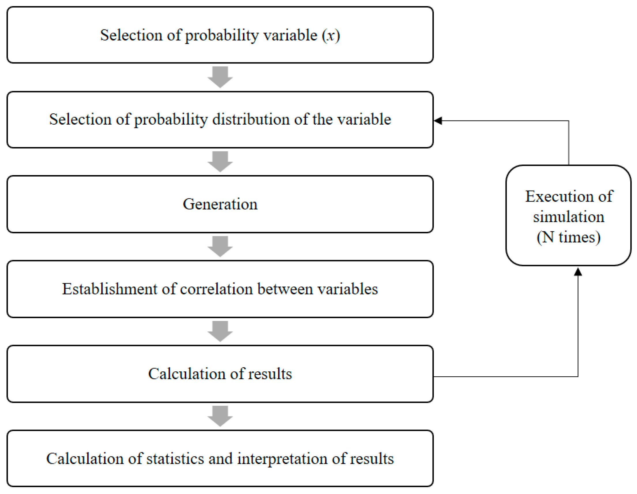
3.2. Stochastic Approach
3.3. Sensitivity Analysis
4. Empirical Results
4.1. Data
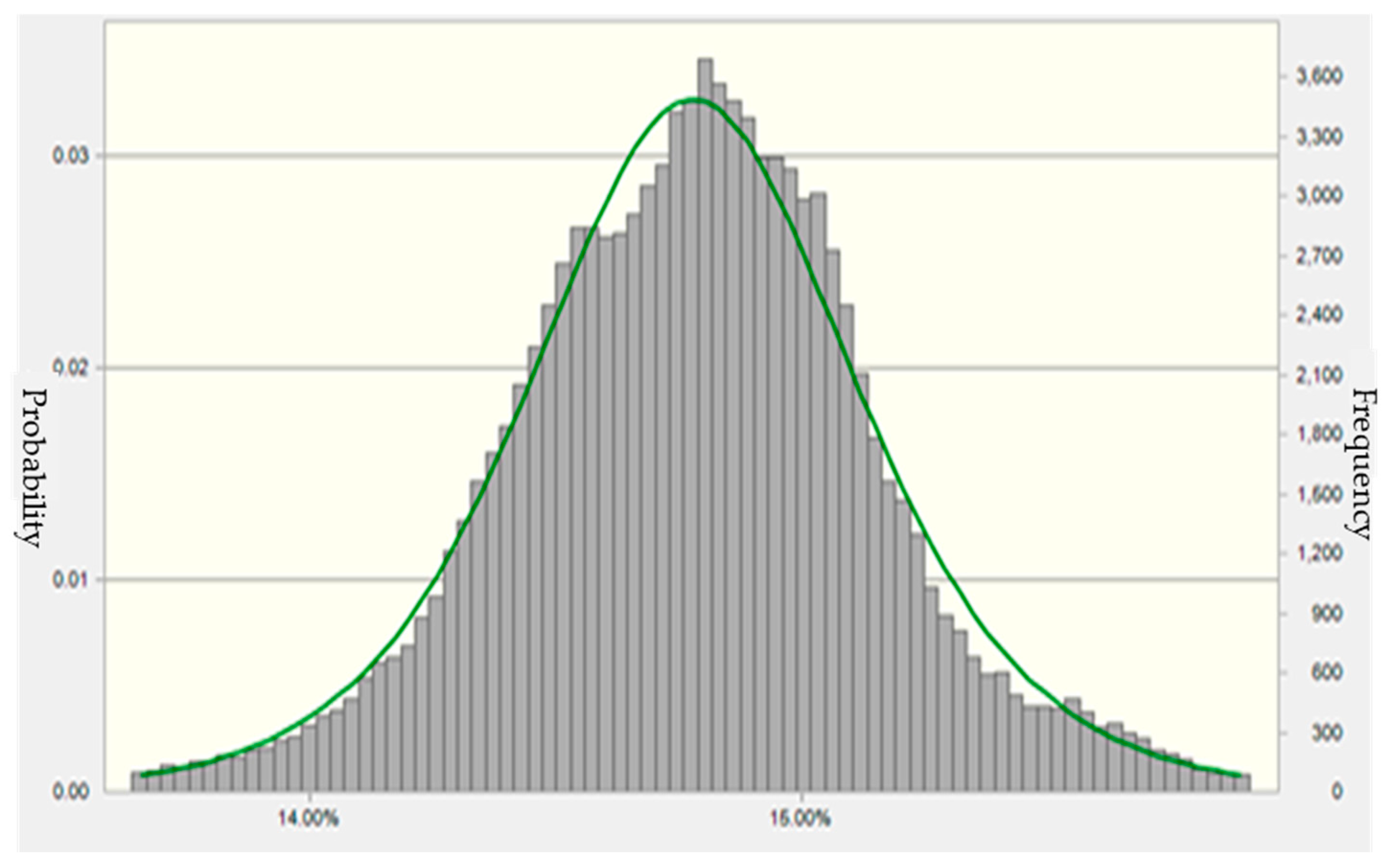
4.1.1. Capacity Factor
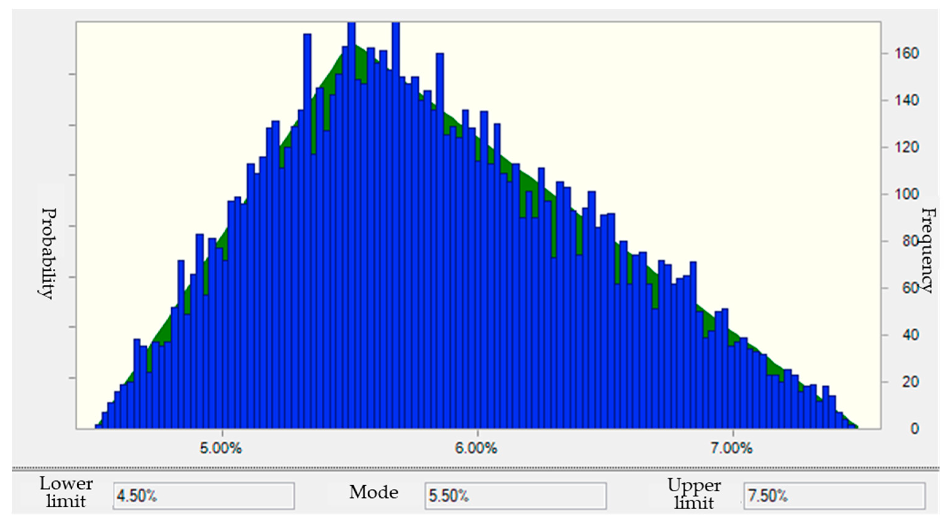
4.1.2. Discount Rate
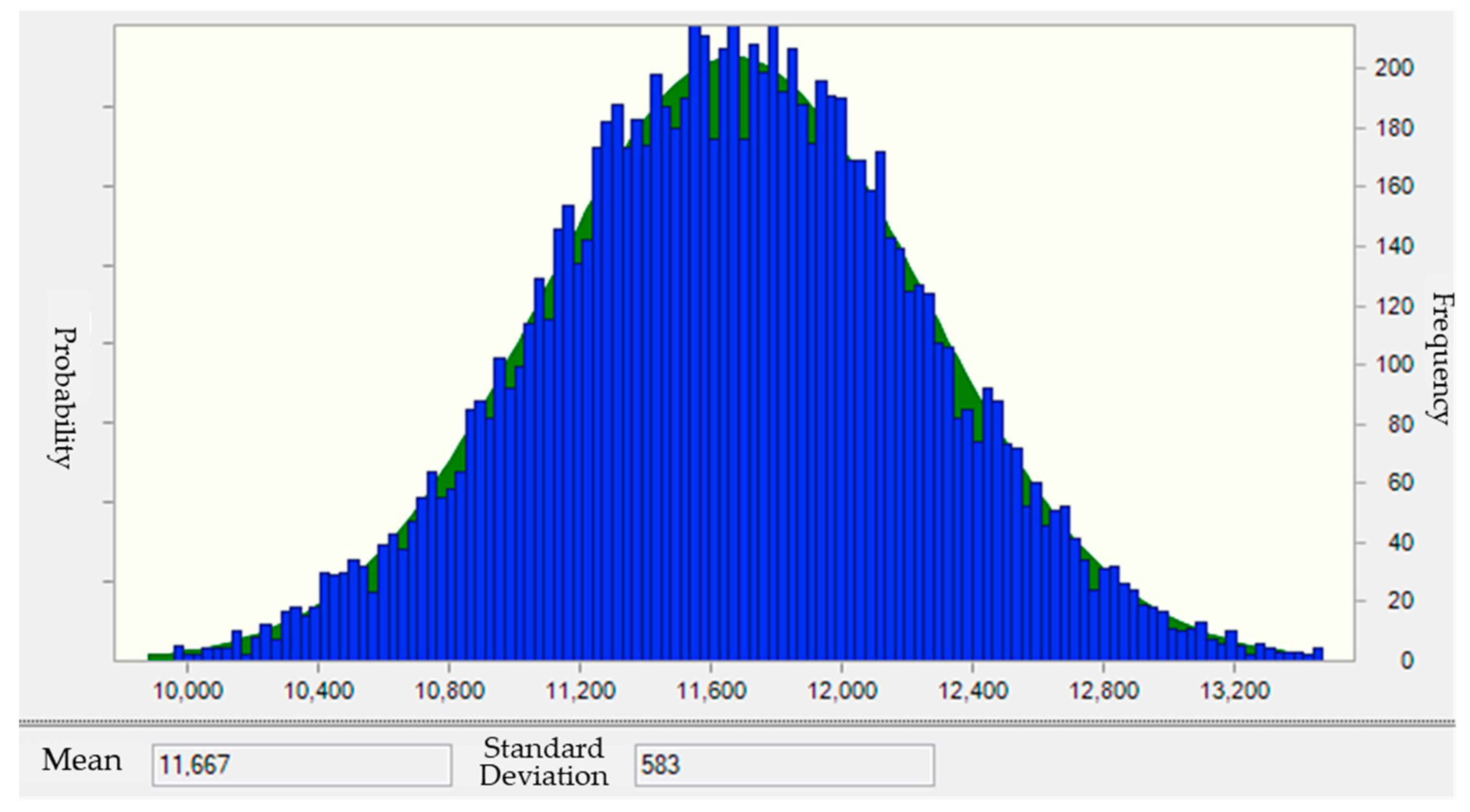
4.1.3. O&M Costs
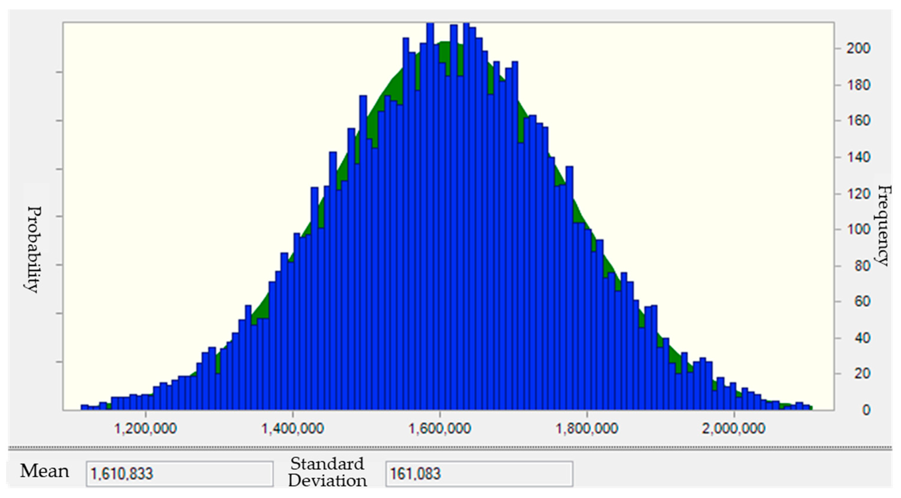
4.1.4. CAPEX
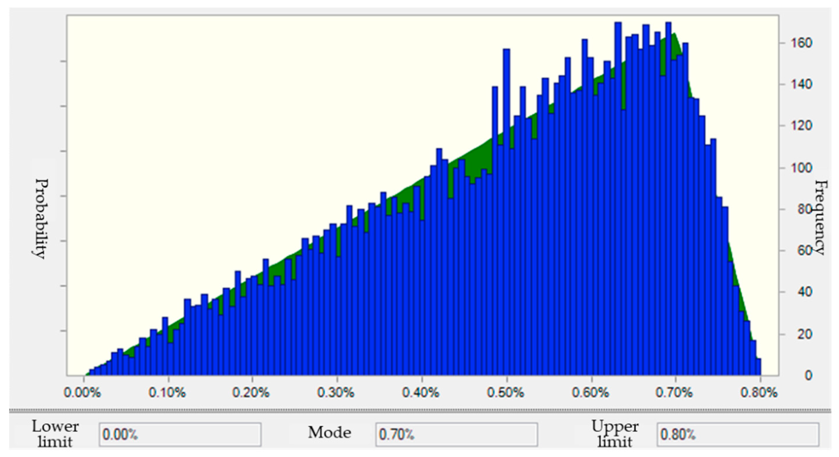
4.1.5. System Degradation Rate
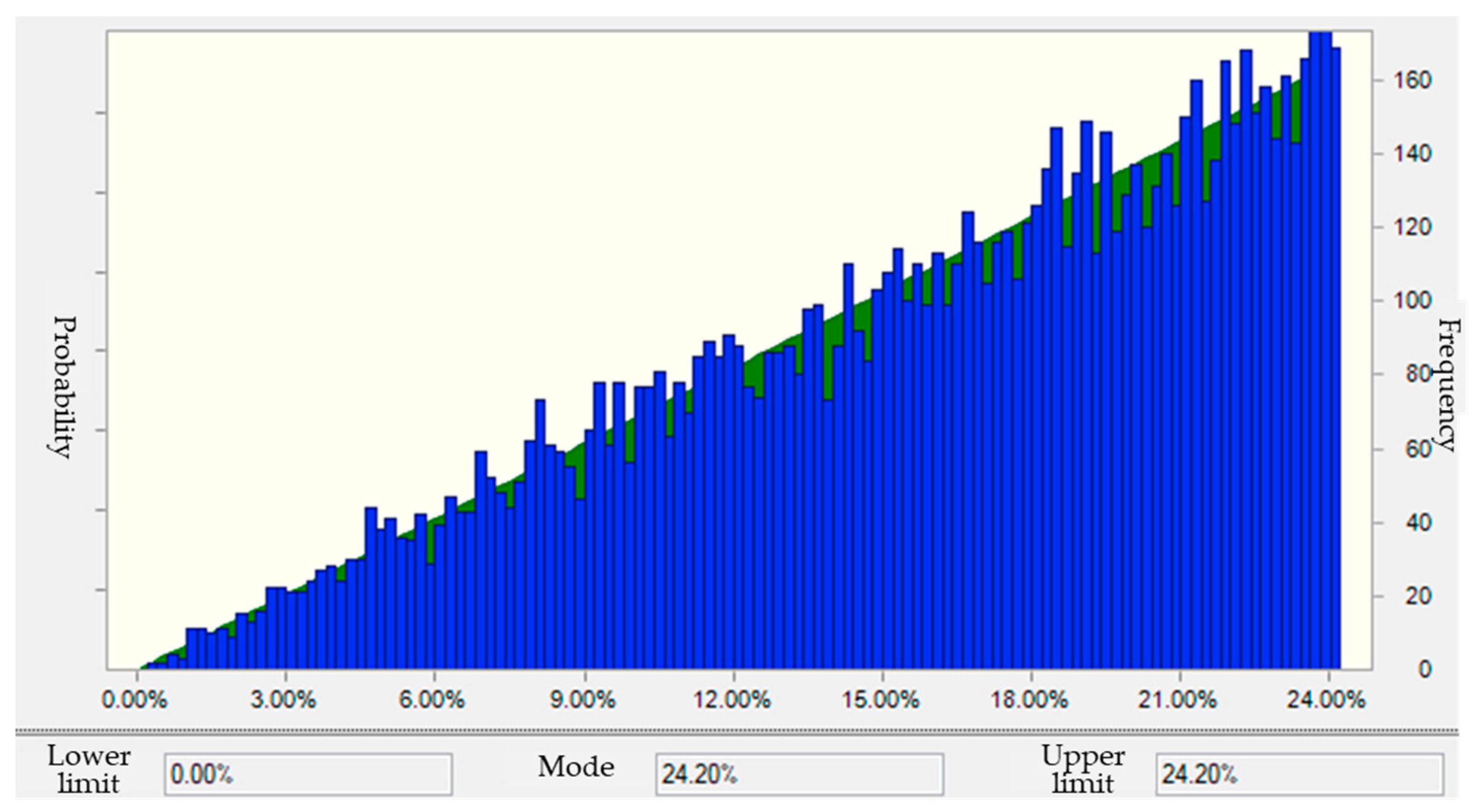
4.1.6. Corporate Tax
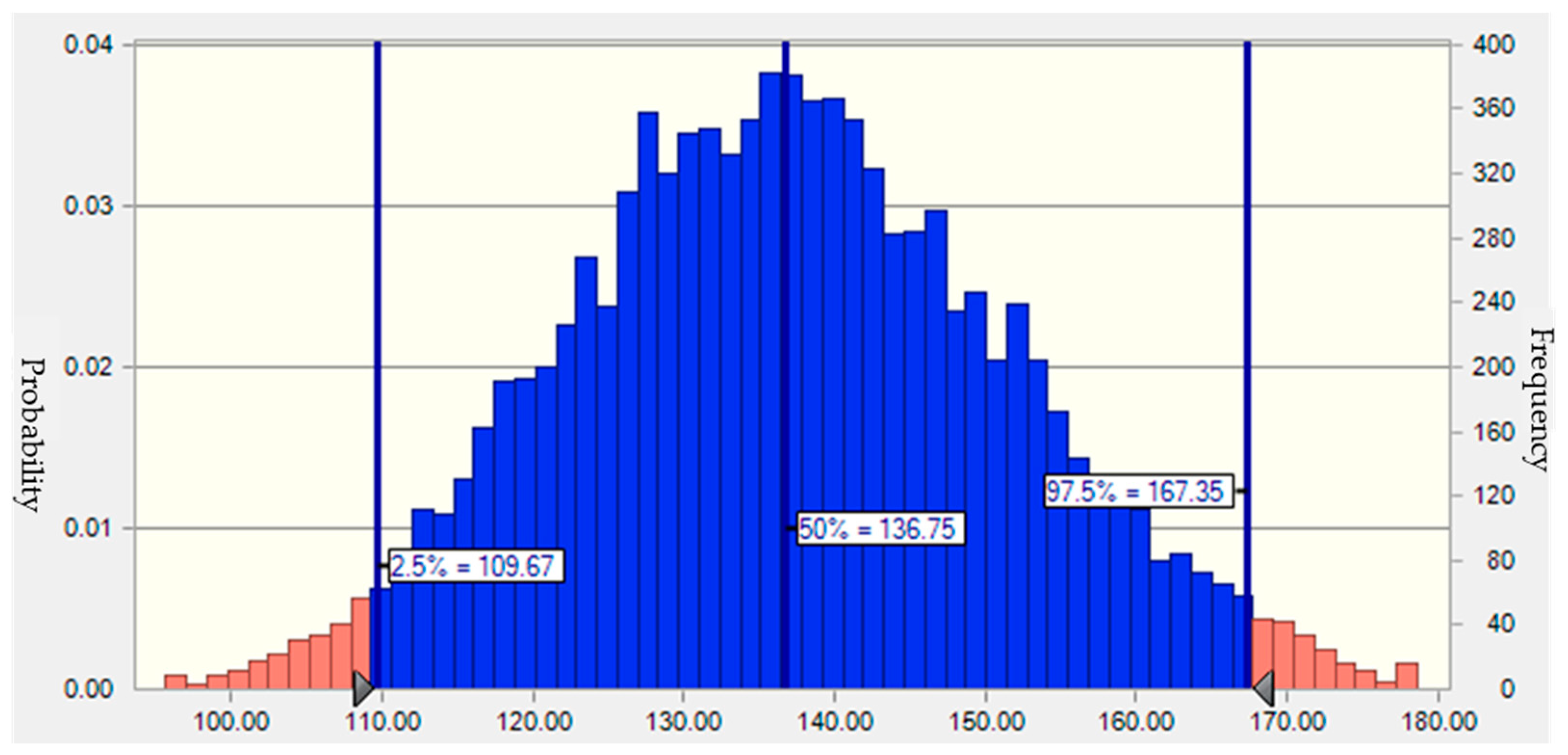
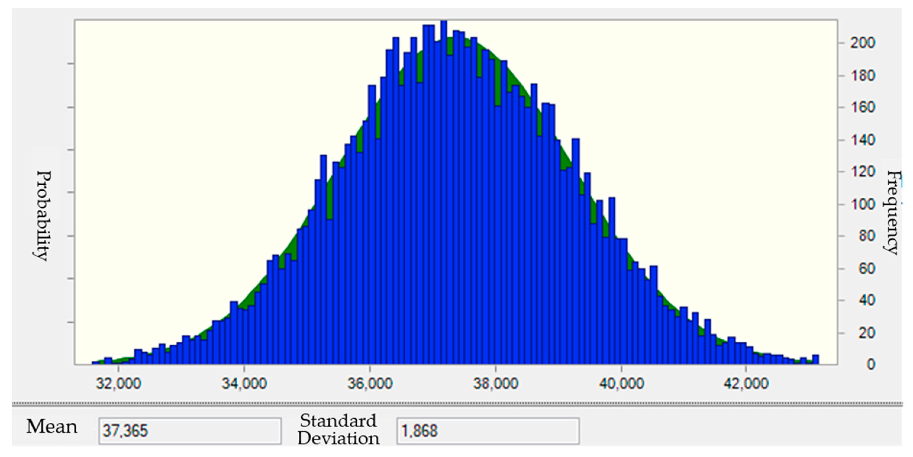
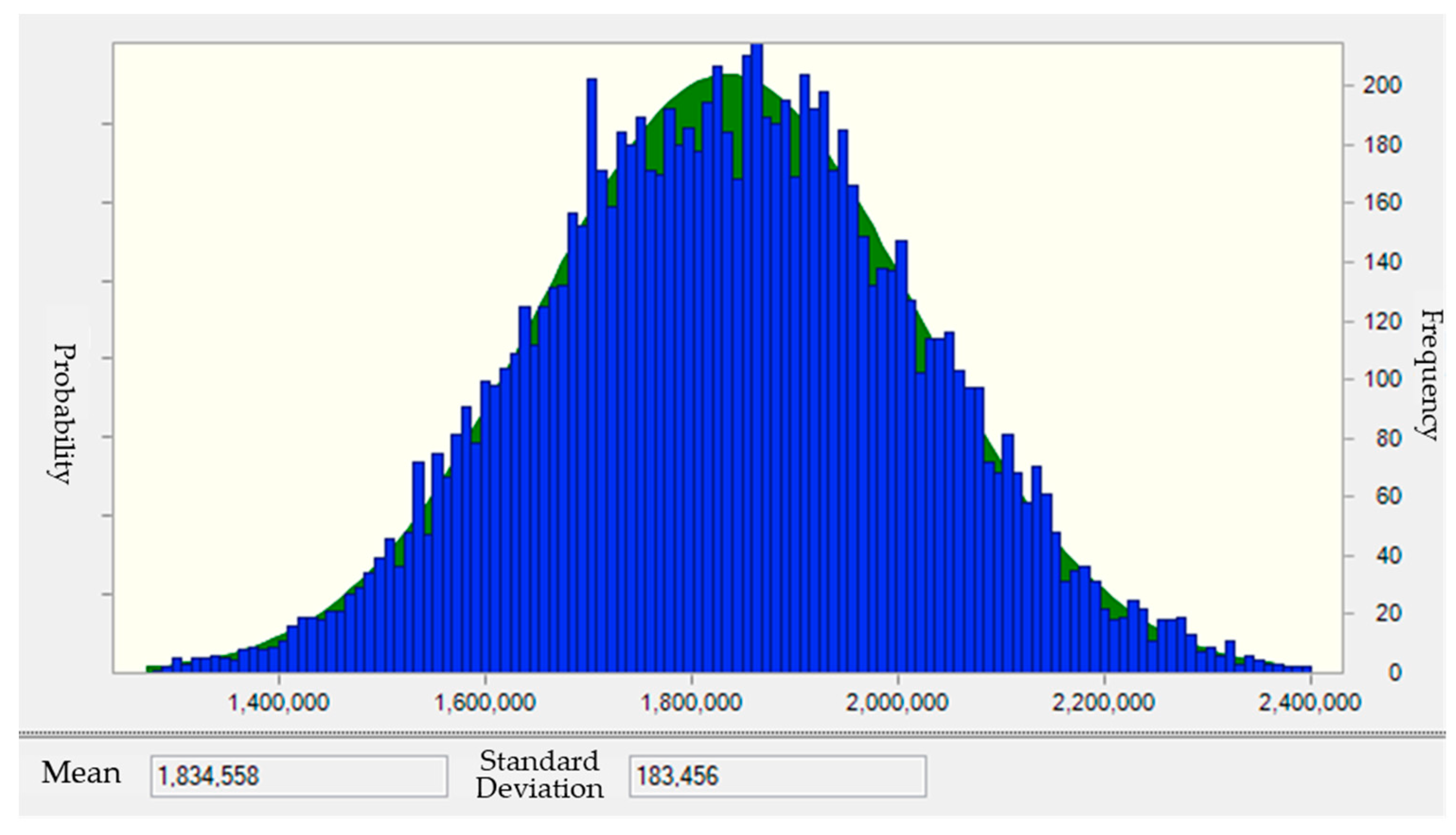
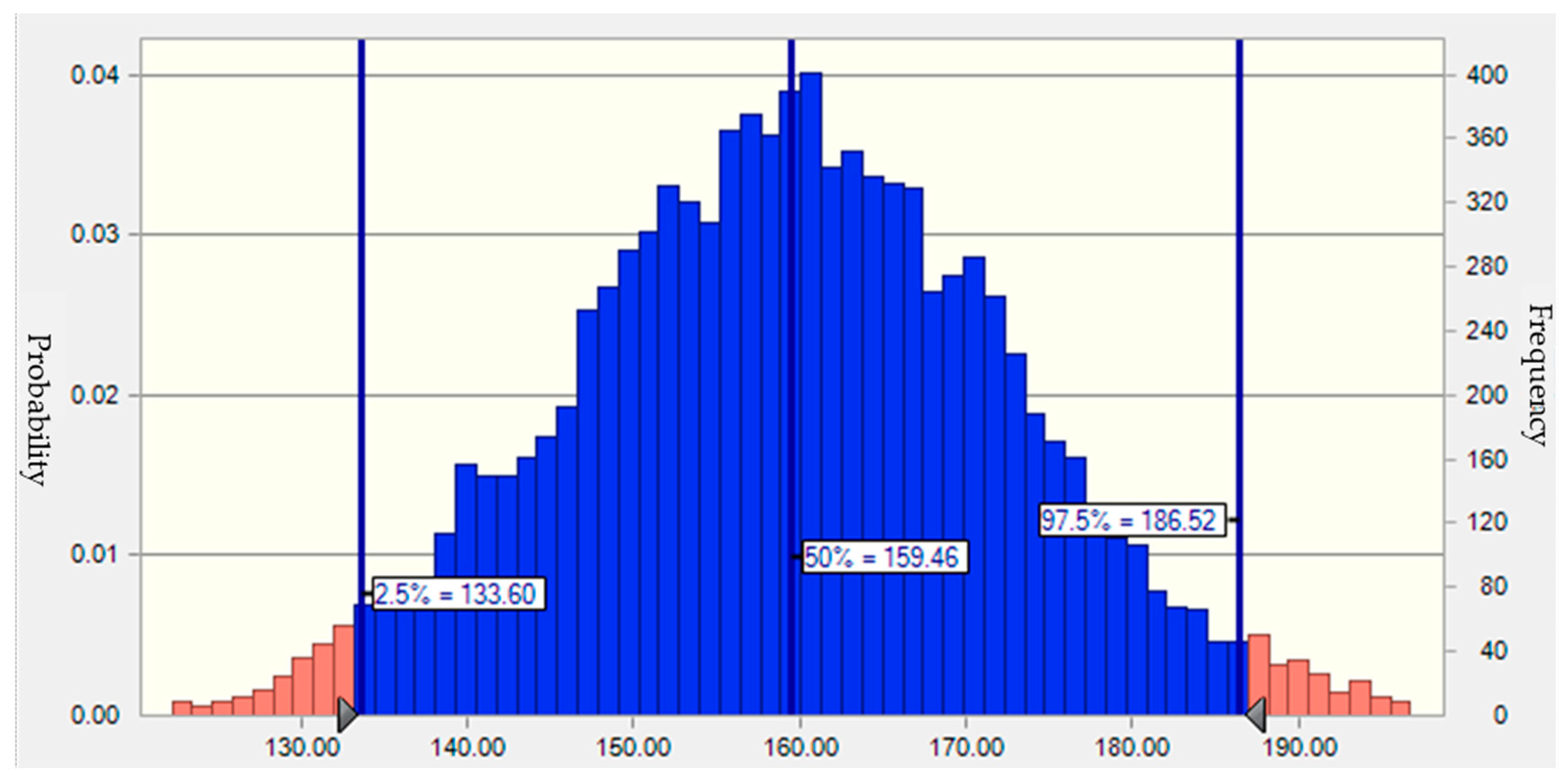
4.2. Results of Stochastic Simulation
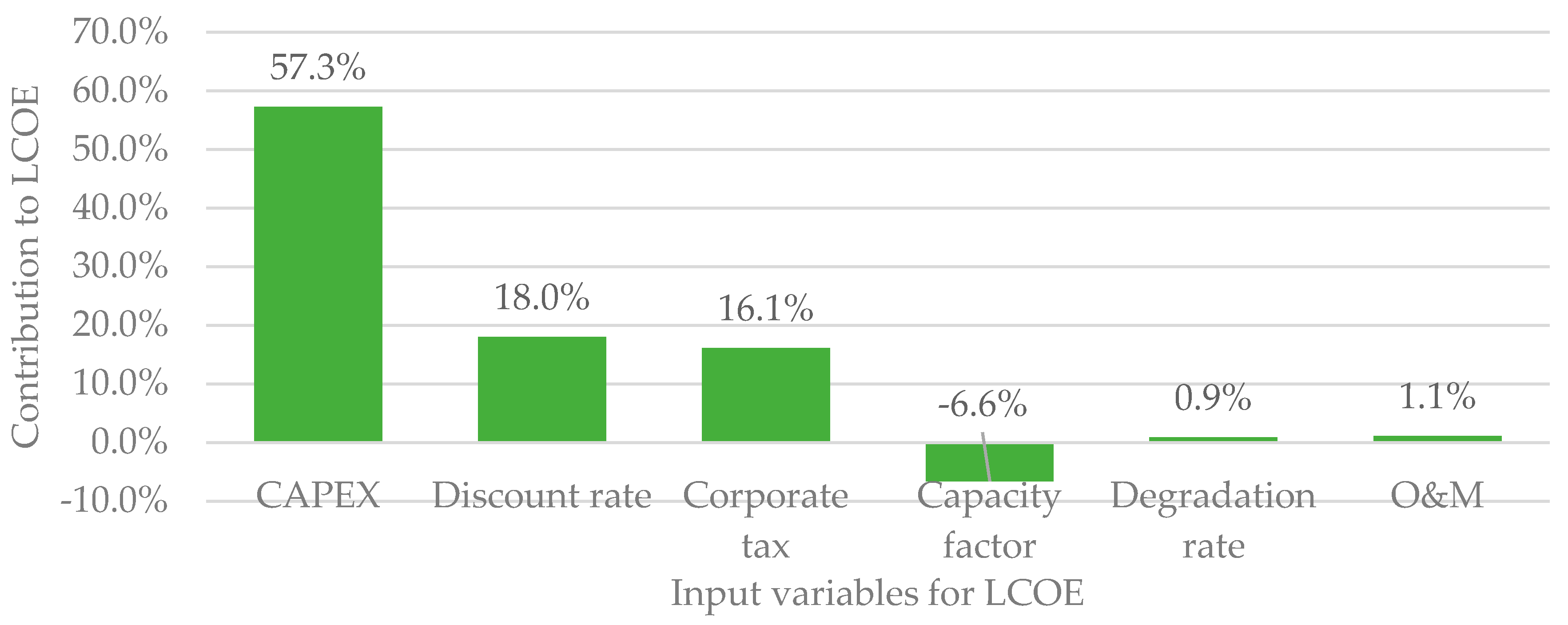
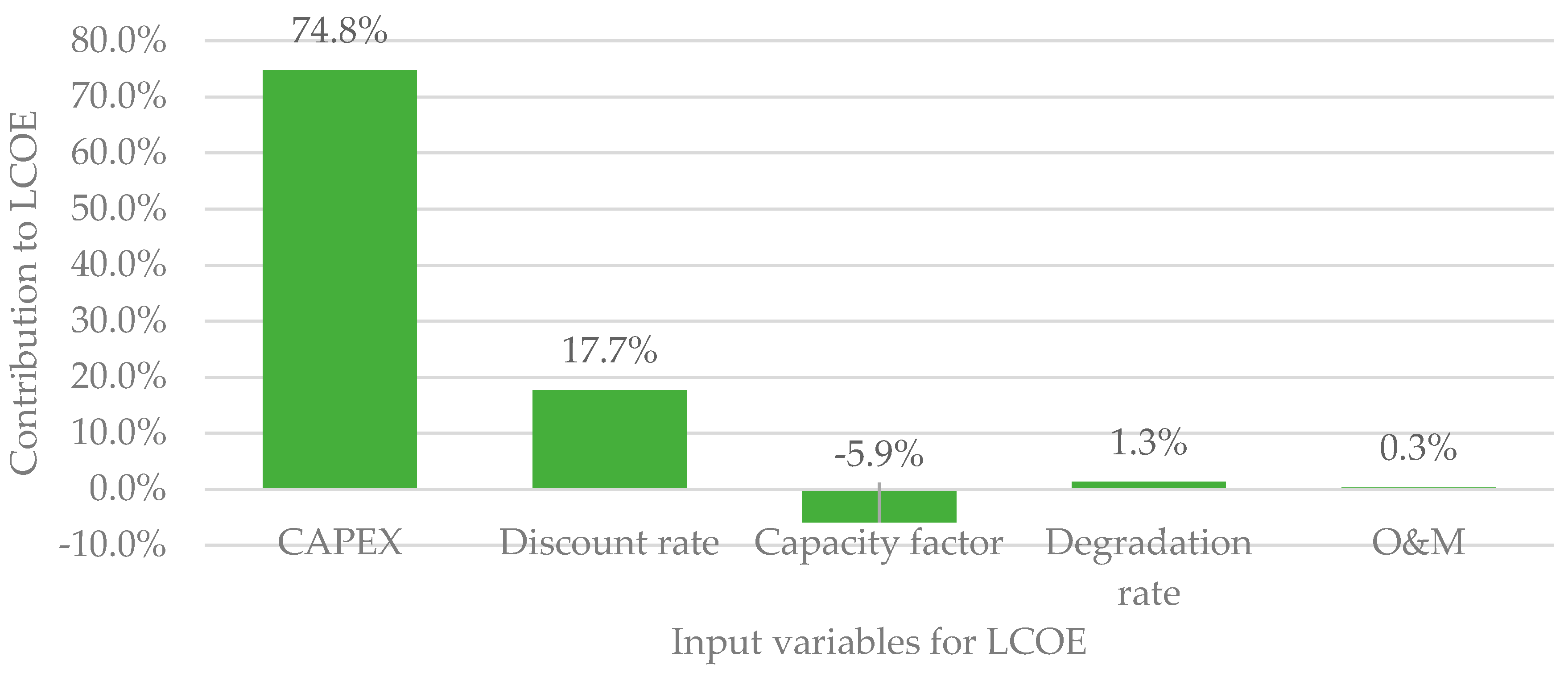
4.3. Sensitivity Analysis Results
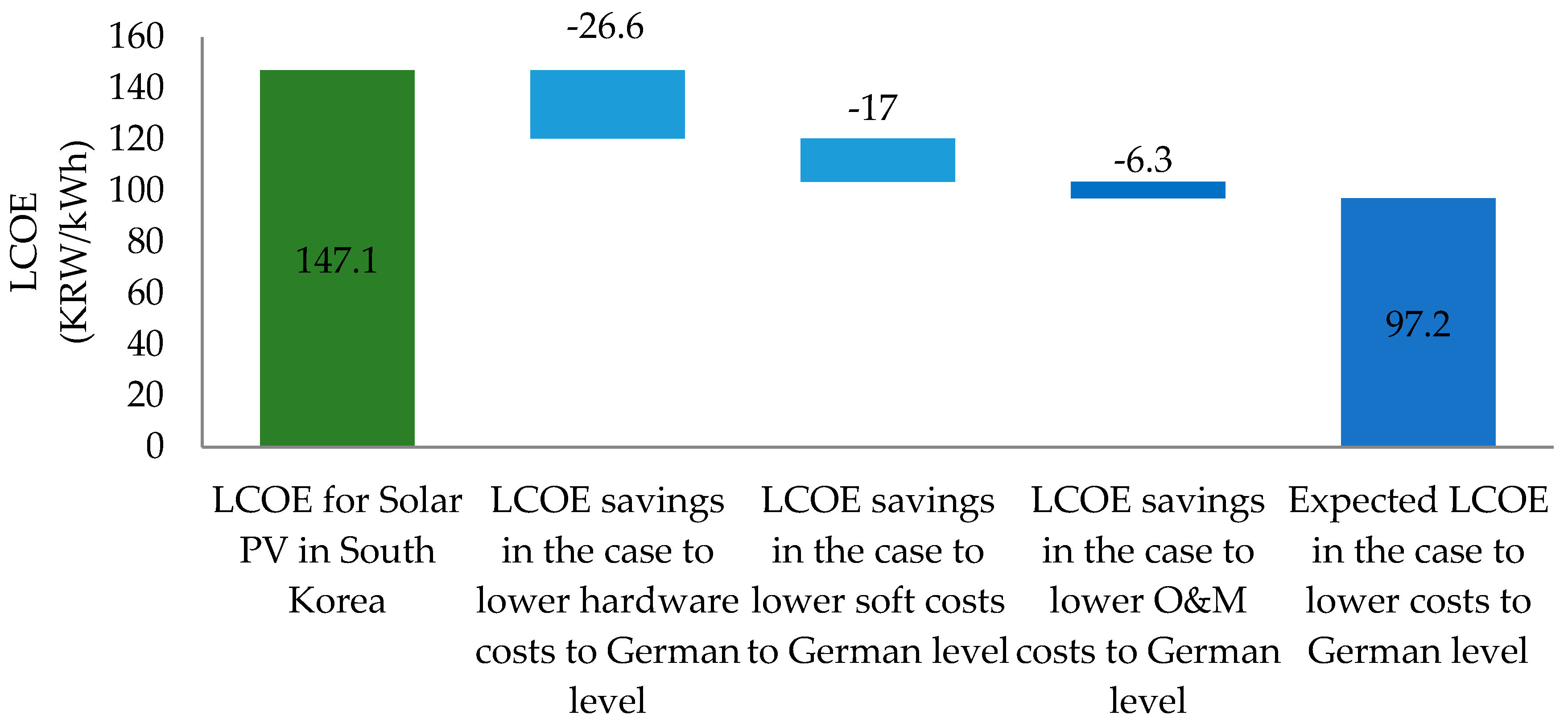
5. Discussion
Author Contributions
Funding
Conflicts of Interest
References
- Olhoff, A.; Christensen, J.M. The Emissions Gap Report 2017: A UNEP Synthesis Report; The United Nations Environment Programme (UNEP) Press: Nairobi, Kenya, 2017. [Google Scholar]
- Hwang, S.-H.; Kim, M.-K.; Ryu, H.-S. Real Levelized Cost of Energy with Indirect Costs and Market Value of Variable Renewables: A Study of the Korean Power Market. Energies 2019, 12, 2459. [Google Scholar] [CrossRef] [Green Version]
- Poulsen, T.; Hasager, C.B.; Jensen, C.M. The role of logistics in practical levelized cost of energy reduction implementation and government sponsored cost reduction studies: Day and night in offshore wind operations and maintenance logistics. Energies 2017, 10, 464. [Google Scholar] [CrossRef] [Green Version]
- Mendicino, L.; Menniti, D.; Pinnarelli, A.; Sorrentino, N. Corporate power purchase agreement: Formulation of the related levelized cost of energy and its application to a real life case study. Appl. Energy 2019, 253, 113577. [Google Scholar] [CrossRef]
- Wang, X.; Kurdgelashvili, L.; Byrne, J.; Barnett, A. The value of module efficiency in lowering the levelized cost of energy of photovoltaic systems. Renew. Sust. Energ. Rev. 2011, 15, 4248–4254. [Google Scholar] [CrossRef]
- Kasperowicz, R.; Pinczyński, M.; Khabdullin, A. Modeling the power of renewable energy sources in the context of classical electricity system transformation. J. Int. Stud. 2017, 10, 264–272. [Google Scholar] [CrossRef]
- Bhandari, R.; Stadler, I. Grid parity analysis of solar photovoltaic systems in Germany using experience curves. Sol. Energy 2009, 83, 1634–1644. [Google Scholar] [CrossRef]
- Branker, K.; Pathak, M.; Pearce, J.M. A review of solar photovoltaic levelized cost of electricity. Renew. Sust. Energ. Rev. 2011, 15, 4470–4482. [Google Scholar] [CrossRef] [Green Version]
- Rhodes, J.D.; King, C.; Gulen, G.; Olmstead, S.M.; Dyer, J.S.; Hebner, R.E.; Beach, F.C.; Edgar, T.F.; Webber, M.E. A geographically resolved method to estimate levelized power plant costs with environmental externalities. Energy Policy 2017, 102, 491–499. [Google Scholar] [CrossRef]
- Clauser, C.; Ewert, M. The renewables cost challenge: Levelized cost of geothermal electric energy compared to other sources of primary energy–Review and case study. Renew. Sust. Energ. Rev. 2018, 82, 3683–3693. [Google Scholar] [CrossRef]
- Chadee, X.T.; Clarke, R.M. Wind resources and the levelized cost of wind generated electricity in the Caribbean islands of Trinidad and Tobago. Renew. Sust. Energ. Rev. 2018, 81, 2526–2540. [Google Scholar] [CrossRef]
- Mundada, A.S.; Shah, K.K.; Pearce, J.M. Levelized cost of electricity for solar photovoltaic, battery and cogen hybrid systems. Renew. Sust. Energ. Rev. 2016, 57, 692–703. [Google Scholar] [CrossRef] [Green Version]
- Nissen, U.; Harfst, N. Shortcomings of the traditional “levelized cost of energy” [LCOE] for the determination of grid parity. Energy 2019, 171, 1009–1016. [Google Scholar] [CrossRef]
- Kore Energy Economics Institute. An International Comparative Analysis on Levelized Costs based on Solar Cost Analysis; KEEI Press: Ulsan, Korea, 2017. (In Korean) [Google Scholar]
- Ragnarsson, B.F.; Oddsson, G.V.; Unnthorsson, R.; Hrafnkelsson, B. Levelized cost of energy analysis of a wind power generation system at Burfell in Iceland. Energies 2015, 8, 9464–9485. [Google Scholar] [CrossRef]
- Castro-Santos, L.; Garcia, G.P.; Estanqueiro, A.; Justino, P.A. The Levelized Cost of Energy (LCOE) of wave energy using GIS based analysis: The case study of Portugal. Int. J. Elec. Power 2015, 65, 21–25. [Google Scholar] [CrossRef] [Green Version]
- Lai, C.S.; McCulloch, M.D. Levelized cost of electricity for solar photovoltaic and electrical energy storage. Appl. Energy 2017, 190, 191–203. [Google Scholar] [CrossRef]
- Kirchem, D.; Lynch, M.A.; Bertsch, V.; Casey, E. Modelling demand response with process models and energy systems models: Potential applications for wastewater treatment within the energy-water nexus. Appl. Energy 2020, 260, 114321. [Google Scholar] [CrossRef]
- Charnes, J. Financial Modeling with Crystal Ball and Excel + Website; John Wiley & Sons: Hoboken, NJ, USA, 2012; Volume 757. [Google Scholar]
- Månberger, A.A.; Stenqvist, B.A. Global metal flows in the renewable energy transition: Exploring the effects of substitutes, technological mix and development. Energy Policy 2018, 119, 226–241. [Google Scholar] [CrossRef]
- Abd Alla, S.; Bianco, V.; Tagliafico, L.A.; Scarpa, F. Life-cycle approach to the estimation of energy efficiency measures in the buildings sector. Appl. Energy 2020, 264, 114745. [Google Scholar] [CrossRef]
- Shi, Y.; Zeng, Y.; Engo, J.; Han, B.; Li, Y.; Muehleisen, R.T. Leveraging inter-firm influence in the diffusion of energy efficiency technologies: An agent-based model. Appl. Energy 2020, 263, 114641. [Google Scholar] [CrossRef]
- Tvaronavičienė, M.; Prakapienė, D.; Garškaitė-Milvydienė, K.; Prakapas, R.; Nawrot, Ł. Energy efficiency in the long run in the selected European countries. Econ. Sociol. 2018, 11, 245–254. [Google Scholar] [CrossRef] [Green Version]
- Adenle, A.A. Assessment of solar energy technologies in Africa-opportunities and challenges in meeting the 2030 agenda and sustainable development goals. Energy Policy 2020, 137, 111180. [Google Scholar] [CrossRef]
- Klaniecki, K.; Duse, I.A.; Lutz, L.M.; Leventon, J.; Abson, D.J. Applying the energy cultures framework to understand energy systems in the context of rural sustainability transformation. Energy Policy 2020, 137, 111092. [Google Scholar] [CrossRef]
- Ahmed, A.; Gasparatos, A. Multi-dimensional energy poverty patterns around industrial crop projects in Ghana: Enhancing the energy poverty alleviation potential of rural development strategies. Energy Policy 2020, 137, 111123. [Google Scholar] [CrossRef]
- Lopez, A.R.; Krumm, A.; Schattenhofer, L.; Burandt, T.; Montoya, F.C.; Oberlaender, N.; Oei, P.-Y. Solar PV generation in Colombia—A qualitative and quantitative approach to analyze the potential of solar energy market. Renew. Energy 2020, 148, 1266–1279. [Google Scholar] [CrossRef]
- Winston, W.L. Simulation Modeling Using@ RISK; Wadsworth Publising Company: California, CA, USA, 1996. [Google Scholar]
- Barreto, H.; Howland, F. Introductory Econometrics: Using Monte Carlo Simulation with Microsoft Excel; Cambridge University Press: Cambridge, UK, 2006. [Google Scholar]
- Spooner, J.E. Probabilistic estimating. J. Constr. Div. 1974, 100. [Google Scholar]
- Alotaibi, R.M.; Rezk, H.R.; Ghosh, I.; Dey, S. Bivariate exponentiated half logistic distribution: Properties and application. Commun. Stat. Theory Methods 2020, 1–23, in press. [Google Scholar] [CrossRef]
- Stein, W.E.; Keblis, M.F. A new method to simulate the triangular distribution. Math. Comput. Model. 2009, 49, 1143–1147. [Google Scholar] [CrossRef]
- Choi, J.; Park, D. An Estimation of the Social Discount Rate for the Economic Feasibility Analysis of Public Investment Projects. J. Soc. Sci. 2017, 43. (In Korean) [Google Scholar]
- Richter, M.; Tjengdrawira, C.; Vedde, J.; Green, M.; Frearson, L.; Herteleer, B.; Jahn, U.; Herz, M.; Kontges, M.; Stridh, B. Technical Assumptions Used in PV Financial Models; International Energy Agency (IEA) Report; IEA Press: Paris, France, 2017. [Google Scholar]


| Solar (Commercial) | Solar (Residential) | |
|---|---|---|
| Standard size | 100 kW | 3 kW |
| CAPEX (100 million won/MW) | Normal distribution (average = 16.1, deviation = 10% of average) | Normal distribution (average = 18.3, deviation = 10% of average) |
| O&M costs (10,000 won/MW·year) | Normal distribution (average = 1167, deviation = 5% of average) | Normal distribution (average = 3737; deviation = 5% of average) |
| Capacity factor (%) | Logistic distribution (average = 14.78, scale = 0.22) | |
| Discount rate (%) | Triangular distribution (minimum = 4.5, mode = 5.5, maximum = 7.5) | |
| Corporate tax (%) | Triangular distribution (minimum = 0, mode and maximum = 24.2) | 0 |
| System degradation rate (%) | Triangular distribution (minimum = 0, mode = 0.7, maximum = 0.8) | |
| Loan interest rate (%/year) | 3.46 | |
| Inflation (%) | 0.97 | |
| Lifespan (year) | 20 | |
| Debt ratio (%) | 70 | |
| Distribution | K-S Statistics (Dn) | Statistics |
|---|---|---|
| Logistic | 0.0147 | Average = 14.78%, Scale = 0.22% |
| Student t | 0.0149 | Intermediate point = 14.78%, Scale = 0.35%, Freedom = 7.28199 |
| Normal | 0.0369 | Average = 14.78%, Standard deviation = 0.41% |
| Log-normal | 0.0369 | Location = −4714.30%, Average = 14.78%, Standard deviation = 0.41% |
| Beta | 0.0376 | Minimum = 9.01%, Maximum = 20.54%, Alpha = 100, Beta = 100 |
| Gamma | 0.0378 | Location = 8.85%, Scale = 0.03%, Form = 207.5021 |
| Weibull | 0.0447 | Location = 13.02%, Scale = 1.91%, Form = 4.92757 |
| Minimum extreme value | 0.0868 | Highest probability = 14.98%, Scale = 0.42% |
| Maximum extreme value | 0.1214 | Highest possibility = 14.57%, Scale = 0.48% |
| BetaPERT | 0.1801 | Minimum = 12.65%, Highest possibility = 14.85%, Maximum = 16.47% |
| Triangular | 0.2268 | Minimum = 12.65%, Highest possibility = 14.85%, Maximum = 16.47% |
| Uniform | 0.3409 | Minimum = 12.66%, Minimum = 16.46% |
| Pareto | 0.4606 | Location = 12.66%, Form = 6.47827 |
| Exponential | 0.5933 | Ratio = 676.83% |
| Statistics | Value | Statistics | Value |
|---|---|---|---|
| Reference value | 165.97 | Kurtosis | 3.04 |
| Average | 159.49 | Variation coefficient | 0.0835 |
| Median value | 159.46 | Minimum | 114.84 |
| Standard deviation | 13.31 | Maximum | 216.08 |
| Variance | 177.29 | Range width | 101.24 |
| Skewness | 0.0647 | Standard error | 0.13 |
| Statistics | Value | Statistics | Value |
|---|---|---|---|
| Reference value | 135.65 | Kurtosis | 2.97 |
| Average | 137.15 | Variation coefficient | 0.1079 |
| Median value | 136.75 | Minimum | 75.77 |
| Standard deviation | 14.80 | Maximum | 197.15 |
| Variance | 219.06 | Range width | 100.56 |
| Skewness | 0.1977 | Standard error | 0.15 |
| Items of Hhardware Costs | KRW | Items of Soft Costs | KRW | Items of O&M Costs | KRW | |
|---|---|---|---|---|---|---|
| Modules | 62,124,000 | License and permits | 9,000,000 | Land lease costs | 1,500,000 | |
| Inverters | 14,375,000 | Standard facility charges | 8,390,000 | Parts replacement costs | Inverters | 718,750 |
| Connection bands | 2,200,000 | Insurance premiums | 1,141,623 | Fuses, etc. | 240,000 | |
| Electric wiring | 601,678 | Supervisory costs | 1,500,000 | Safety management costs | 1,277,760 | |
| Structures | 5,895,677 | Other expenses | 5,136,649 | Total | 3,736,510 | |
| Installation construction costs | 23,933,435 | Design costs | 1,500,000 | |||
| Total | 109,129,790 | General management costs | 6,924,483 | |||
| Profits | 5,570,428 | |||||
| Total | 39,163,183 | |||||
© 2020 by the authors. Licensee MDPI, Basel, Switzerland. This article is an open access article distributed under the terms and conditions of the Creative Commons Attribution (CC BY) license (http://creativecommons.org/licenses/by/4.0/).
Share and Cite
Lee, C.-Y.; Ahn, J. Stochastic Modeling of the Levelized Cost of Electricity for Solar PV. Energies 2020, 13, 3017. https://doi.org/10.3390/en13113017
Lee C-Y, Ahn J. Stochastic Modeling of the Levelized Cost of Electricity for Solar PV. Energies. 2020; 13(11):3017. https://doi.org/10.3390/en13113017
Chicago/Turabian StyleLee, Chul-Yong, and Jaekyun Ahn. 2020. "Stochastic Modeling of the Levelized Cost of Electricity for Solar PV" Energies 13, no. 11: 3017. https://doi.org/10.3390/en13113017
APA StyleLee, C.-Y., & Ahn, J. (2020). Stochastic Modeling of the Levelized Cost of Electricity for Solar PV. Energies, 13(11), 3017. https://doi.org/10.3390/en13113017