Abstract
A novel optimization strategy is proposed to achieve a reliable hybrid plant of wind, solar, and battery (HWSPS). This strategy’s purpose is to reduce the power losses in a wind farm and at the same time reduce the fluctuations in the output of HWSPS generation. In addition, the proposed strategy is different from previous studies in that it does not involve a load demand profile. The process of defining the HWSPS capacity is carried out in two main stages. In the first stage, an optimal wind farm is determined using the genetic algorithm subject to site dimensions and spacing between the turbines, taking Jensen’s wake effect model into consideration to eliminate the power losses due to the wind turbines’ layout. In the second stage, a numerical iterative algorithm is deployed to get the optimal combination of photovoltaic and energy storage system sizes in the search space based on the wind reference power generated by the moving average. The reliability indices and cost are the basis for obtaining the optimal combination of photovoltaic and energy storage system according to a contribution factor with 100 different configurations. A case study in Thumrait in the Sultanate of Oman is used to verify the usefulness of the proposed optimal sizing approach.
1. Introduction
Optimal sizing of hybrid renewable plants is essential for utilizing the available resources effectively while at the same time avoiding under- or overestimating the size of the power plants. The intermittent nature of wind speed and solar irradiation mandates the use of optimization methodologies to exploit the complementary nature of wind and solar power sources in a way to mitigate output power fluctuations. Hybrid plants of wind and solar make the system more reliable and robust and reduce the required energy storage systems (ESS) instead of using each source individually [].
Different sizing techniques for determining the size of hybrid plants of wind, solar, and battery (HWSPS) were investigated in previous studies. Cost and reliability are the most used criteria for determining the optimum combinations of wind and photovoltaic (PV) energy []. Effective sizing of the system is essential for meeting the load demand profile in a way that yields reliable and cost-effective hybrid renewable systems []. Therefore, the sizing of HWSPS must be justified economically and technically. Based on previous research, the most applied sizing algorithms are intuitive, numerical iterative, and analytical algorithms. An intuitive algorithm is simple to use but cannot make a quantitative link between cost and reliability []. In contrast, an analytical method is simple to use and at the same time can present a relationship between capacities and reliabilities []. However, a numerical iterative algorithm (NIA) can give an accurate reliability analysis but needs longer-term time-series data and more computational time []. In [], a summary was given of the most applied optimization techniques in sizing the HWSPS, which are graphic construction, probabilistic methods, NIA, and artificial intelligence (AI). Graphic construction and probabilistic algorithms have lower complexity and need more computational time. However, the NIA and AI algorithms have higher accuracy than the other algorithms.
Rajkumar et al. [] presented a dynamic programming model, which was used to obtain the optimal loss of the power supply probability (LPSP) and the cost of energy (COE) of a hybrid solar incorporating battery (BESS) and an auxiliary wind plant. A similar idea was implemented in [] using a hybrid genetic algorithm with particle swarm optimization (GA-PSO) by minimizing the total present cost and by taking LPSP as a reliability factor. Additionally, Bilal et al. [] used a multi-objective genetic algorithm to optimize two antagonistic objectives: the annualized cost of the system and LPSP. Chong et al. [] studied the techno-economic feasibility for different combinations of wind, PV, and BESS sources. The analysis was carried out for small household loads with average monthly wind speed and solar radiation. It was concluded that the net present cost (NPC) of the HWSPS is lower than the NPC of the PV/BESS or the wind/BESS. However, the input data for this feasibility study were taken for a wide timescale, which leads to lower accuracy of the results.
Complexity of the selected terrain has a significant impact in the optimization of the wind farm []. In addition, variability in both the renewable resources’ output power and the load demand profile makes the decision of sizing renewable resources more complex. Mixed-integer linear programming (MILP) was used in [] to minimize the levelized cost of energy (LCOE) to size and schedule the off-grid hybrid resources that integrate wind, PV, diesel, and BESS in a way to meet the energy demand. However, the daily demand was assumed to be the same every day of the year, which does not reflect the real trend of the demand profile.
In [], the NIA was used to optimize the capacities of HWSPS using the deficiency of power supply probability and the levelized unit electricity cost to evaluate the technical and economic aspects of the HWSPS. However, the load profile was assumed to follow the same trend every day of the year, which is not true for real load profiles. Another NIA was presented by [] to obtain the optimal HWSPS using the LPSP to assess the system’s reliability. The constraints used were the number of PV modules and the size of the wind turbine to minimize the life cycle cost of the plant. In addition, the authors in [] optimized the HWSPS based on NIA in two steps. The first step was carried out to determine the possible combinations of wind and PV to get the optimal maximum value. In the second step, the BESS was determined based on the reliability to cost ratio.
In all the studies mentioned, the sizing approaches focus on optimizing the size of HWSPS by minimizing the cost in a way to guarantee the required reliability of power supply. The reliability was taken to measure the compliance of the generated power with the demand profile. Smoothing of wind power output is also one of the concerns to keep the output power more reliable. Power smoothing methods are categorized into methods based on energy storage (indirect methods) and methods that are not based on energy storage (direct methods) []. Indirect methods use energy storage systems such as BESS due to its fast dynamic response []. The BESS is normally used to compensate for the required supply or to absorb power to make the system stable and within operational limits [].
In some studies, mathematical smoothing techniques are used to generate a reference power line. Some of these techniques are moving average (MAV) [], double moving average [], moving median, exponential moving average (EMA) [], and wavelet decomposition []. The smoothness is adjusted by manipulating the window size as done in [] while using double MAV for PV output power. In addition, the EMA of wind power was used as a reference output power in []. Moreover, the authors in [] used the MAV to mitigate fluctuations in solar PV output. In [], the averaged output powers of PV and wind were used as a reference to determine the BESS capacity. The BESS capacity in [] was defined based on the MAV of PV output power. The authors in [] used two predetermined BESS capacities, one designed for energy and the other for power smoothing, depending on the reference PV power produced from MAV and a low-pass filter. A hierarchal MAV was also utilized in [] to get an optimal utilization of BESS that needed to mitigate the fluctuations in PV output power. The studies reveal the ability of MAV to filter out power fluctuations and generate a reference power line.
According to the literature on the sizing of HWSPS, none of the studies include the wake effect in the sizing of HWSPS. Thus, this study will include a model of the wake effect in the sizing of HWSPS to reduce the wind power losses due to the turbines’ layout. Furthermore, the MAV of wind power is used to generate a smooth reference power within the operational ramping rates instead of using the load demand profile to build an HWSPS. The PV and BESS are sized to fulfill the generated reference power. Thus, an integrated approach is developed to get an optimal size of HWSPS using a genetic algorithm with a numerical iterative algorithm (GA-NIA).
This paper is organized as follows: Section 2 introduces the models of the wind turbine, PV, and BESS that are used in the proposed approach. Section 3 presents an energy management strategy. The optimal HWSPS sizing approach is described in Section 4, while Section 5 comprises the techno-economic modeling to evaluate the produced configurations of HWSPS. Section 6 provides the data of the case study that is used in the proposed approach. The results and discussion are presented in Section 7. Finally, Section 8 concludes the paper.
2. Modeling of Power Sources
The hybrid system is implemented using three power sources which are wind turbine, PV source, and BESS. Modeling of the sources is a pro-active step in the sizing of HWSPS. A description of each source’s model is described in the below subsections.
2.1. Wind Turbine Model
Calculating the energy harvested from a wind farm is highly linked to the installed wind turbine. In most studies, such as [], power equations were used to calculate the wind farm’s output power. It is more precise to linearly interpolate the output power from the power curve of the wind turbine’s manufacturer at each input wind speed. In this study, 3.83-MW wind turbines are used in the wind farm. The output power () is the total yield production of the turbines. Figure 1 shows the curves of a wind turbine, including the output power, thrust coefficient , and power coefficient .
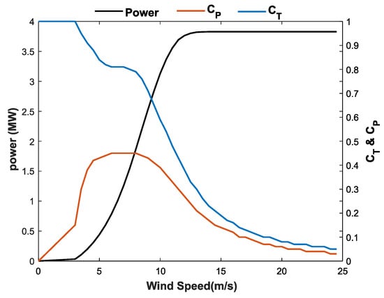
Figure 1.
Power curve of a 3.83-MW wind turbine.
2.2. Photovoltaic Generation Model
The solar power of a PV plant is a function of global horizontal irradiance (GHI) and the ambient temperature in the panel, as given in [,]. In this study, a polycrystalline PV is used, and the solar output power at each time instant for each PV module is calculated by Equation (1):
where , , , , , , and are the derating factor, the module’s rated power, the module’s temperature coefficient of power, the module’s temperature at time t, the temperature at the standard test condition , the irradiance at time t, and the irradiance level at , respectively.
2.3. Energy Storage Model
BESS is needed to enhance the HWSPS stabilization as well as to store energy and supply power when needed. The BESS is sized in a way to mitigate the reference power during shortage or non-availability of wind power or solar power . The BESS state of charge is determined according to the wind and solar energy production and reference power, as well as the battery charge and discharge rate, which is in this study.
The states of charge and discharge of BESS are calculated as in [] by defining the BESS energy using Equations (2) and (3), respectively:
where , , and are the hourly self-discharge rate, the efficiency of the inverter, and the battery (charge/discharge) efficiency, respectively.
At each time instant , the battery’s is subject to the following constraints:
where the minimum state of charge is defined using the battery’s depth of discharge , and the maximum state of charge takes the value of the battery’s bank capacity . A battery with a nominal capacity of 2000 and a charge efficiency of is used in this study [].
3. Energy Management Strategy
The proposed power flow model is based on three cases that depend on the power difference between the reference power and the generation of wind and PV. The proposed cases are illustrated in Figure 2 and are as follows:
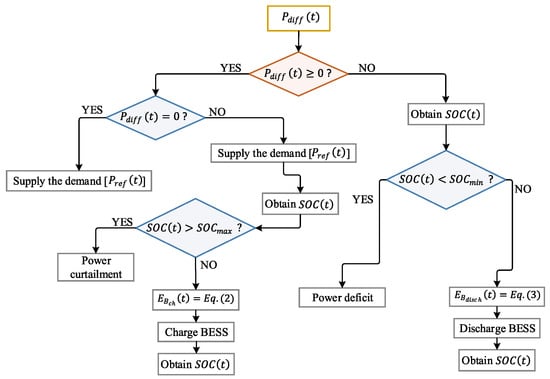
Figure 2.
Energy management strategy.
- Case :In this case, all the generated PV and wind powers are equal to the smoothed reference power. Thus, the curtailed and deficit power values are equal to zero:
- Case :The power generated is more than , the excess power transferred to charge the BESS, and this depends on the battery’s . If the BESS is fully charged, then the excess power will be curtailed. The deficit power, in this case, is equal to zero. The limits of BESS charge power are given in Equation (8):
- Case :This case uses the BESS to cover the needed supply due to the shortage in the generated power from PV and wind. The discharged power from the battery depends on , as illustrated in Equation (9):
In case the BESS cannot cover the needed supply, then the value is equal to or less than , which depends on the battery’s .
4. Optimal Sizing Methodology
Due to the objective to get an optimal combination of wind, PV, and BESS, the study developed a methodology to get an optimal HWSPS. It involves some factors like the wake effect model to reduce the power losses in the wind farm. In addition, the smoothing technique is used to mitigate the output fluctuations. Hence, the following subsections described the optimal HWSPS sizing approach.
4.1. Wind Farm Sizing
The sizing approach utilizes the actual recorded data for wind speed and solar irradiance with the optimization techniques to size a suitable wind and PV plant capacity. This approach is applicable on the site that has rich wind resources with abundant solar irradiance to make use of the complementary nature of the wind and PV resources. Thus, sizing of a wind farm is the primary objective in this study, and it is the basis for determining the sizes of PV and BESS. A genetic algorithm is used to get the optimal wind farm size. The methodology depends on the dimension of the selected site, the location of the turbines, and the wind speeds and directions. Wind power changes, with little variation in wind speed, due to the cubical proportionality between them []. Thus, the wake effect model is deployed to reduce the power losses due to the wind turbines’ layout in the farm. The wake effect means that there is a speed reduction in the wind speed reaching upstream turbines due to the downstream turbines. This effect is induced as a reduction in wind speeds reaching downstream turbines. Jensen’s wake effect model is one of the models that is widely used due to its simplicity and relatively good accuracy [].
To illustrate the idea of Jensen’s model, Figure 3 shows three hypothetical wind turbines. is totally inside the wake of , but is partially affected by the wake of . The wind turbine is affected by the wake effect if one of the conditions mentioned in Equation (10) is met:
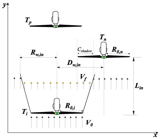
Figure 3.
Illustration of the wake effect of on and (top view of the wind farm).
For partial shadowing, only a percentage of the turbine’s affected area to the wind turbine’s swept area is taken. Thus, only the affected area of is considered in calculating the wake effect due to , as given by Equation (11):
where
Accordingly, the wind speed that reaches can be calculated by taking the summation of the wake effects of the other turbines []:
where
The histograms of wind speeds and directions are the significant inputs to get the optimal output power of the wind farm in a way to reduce the wake effect among the turbines. The main idea in this study is to get the number of turbines that can be allocated in the selected site. It is an optimization problem that produces the coordinates of the turbines’ cells to get the minimum value of the objective function. The selected site of 2000 m × 2000 m is divided into a grid of cells, with a cell size of 200 m × 200 m, in which turbines can be located in the center of the cells. Thus, the total number of variables is 100, representing each cell in the grid.
This wind farm layout optimization (WFLO) problem has technical and cost restrictions. The objective is to minimize the cost of energy (COE). The WF’s power output for each wind scenario is weighted by the scenario’s probability , and the expected power output is incorporated in the optimization objective. This section represents the WFLO model to get the minimal cost of energy as a function of the WT’s numbers and locations. The WFLO model is presented mathematically in Equations (13)–(17):
subject to
The nominator of the objective function in Equation (13) represents the economies of scale in wind farms with a constant term and a variable term []. The variable term indicates the inverse relationship with the number of wind turbines. In addition, the denominator is to get the average annual energy generated, which is equivalent to calculating the power since the number of hours per year that a wind farm produces electricity is considered to be constant. Integrating the wind speed from zero to infinity is similar to integrating between cut-in and cut-out speeds. The constraint of the farm’s boundaries, as stated in Equations (14) and (15), ensures placing the wind turbines within the specified area, which is a realistic constraint for most layout problems. In addition, the minimum spacing between wind turbines is set to be five times the turbine radius, as represented in Equation (16). Moreover, the constraint in Equation (17) is to enforce the number of turbines to be greater than zero. The optimization uses 600 populations with 1000 generations to evaluate the fitness value. The optimization process stops when the improvement in the fitness value has been below a threshold for a number of consecutive steps or if the maximum number of generations is reached.
4.2. Smoothing Model
Smoothing of is important in defining the optimal operational policies to limit the ramp rates. Limiting of the generation ramp rate should be addressed carefully to ensure mitigating the output power variability. The ramp rate indicates a power change event in a specific time interval. The ramp rate could be ramp-up (positive) or ramp-down (negative) []. It can be supported by power curtailment in the ramp-up rate and limiting the ramp-down rate using the reserve services. Limiting the ramping is crucial for protecting renewable plants and for regulating them easily by other conventional power plants [].
In this study, the moving average smoothing method (MAV) is used to get a smoothed reference output power , which represents the load demand. The value of is the reference for determining the optimal HWSPS plant.
According to the literature [,,], MAV is mainly used to generate a smoother output. The period utilized in MAV to get the value is significant. Thus, the value of k must be defined in a way to reach the desired ramping rate and at the same time to avoid over-smoothing of the output power and to keep the ramping within the grid codes regulations. In general, the value of k depends on the wind profile and the grid codes in the selected site. In this study, the ramping is limited to of the wind farm’s rated power in a 10-min time window. The mathematical representation of the k-period MAV is given by Equation (18):
The power fluctuation is measured at each time instant, taking the difference between the subsequent output powers, as stated in Equation (19):
4.3. Sizing of the Photovoltaic and Battery
The main purpose of utilizing PV and BESS is to get a smoother output power. The optimal size of the wind farm is fixed as determined in Section 4.1. To get the optimal combination of PV and BESS in a wind farm, NIA has been employed. First of all, the output power of each PV module was calculated by using Equation (1). Then, a contribution factor is defined from 0 to 1, with an increment of 0.01, to get the size of the PV plant. The purpose of using a contribution factor is to determine a range for the search space. Some authors [] utilized a saturation factor to size the PV and wind plants with an increment of 0.02. However, in this paper, the determination of PV size is calculated using Equation (20) with 100 different solutions. When , there is no need for PV power, and means that the power generated by the PV plant is equal to . Accordingly, there are 100 configurations of PV and BESS in the defined search space:
After getting the number of PV modules , BESS is sized based on the cumulative net energy according to Equation (21). By the way, BESS can provide efficient power smoothing without PV but with positive cost implications []. Thus, in this study, the BESS is operated as a second source for smoothing purposes to reduce its capacity as well as to maintain the cost of the system:
where
A positive value of means that the BESS is in charge mode, and a negative value that it is in discharge mode. To avoid oversizing of BESS, the value of is zero for positive .
A negative is considered only for determining the BESS capacity since the purpose of BESS is to mitigate any shortage in the generation instead of storing all excess power.
Therefore, the minimum value of for the whole time-series data are used to determine the capacity of BESS for each configuration, as stated in Equation (22):
5. Techno-Economic Modeling
The primary objective of the integrated approach is to size the HWSPS to get a cost-effective and reliable system. Reliability and system cost analysis plays a vital role in evaluating the HWSPS size. Therefore, the following subsections explain the techno-economic modeling to evaluate the produced configurations of HWSPS.
5.1. Cost of Energy
The COE is a key performance indicator for evaluating the proposed HWSPS. Therefore, the calculation of the COE of all the 100 configurations of wind, PV, and BESS is conducted to get the minimal COE.
The COE is used to rank the optimal combinations of wind, PV, and BESS that satisfy the specified constraints. It is defined by getting the capital costs of the generation units in the plant , the operation and maintenance cost , the replacement cost , and the salvage costs divided by the total energy generated. The main technical and economic parameters used in this study for the PV module, wind turbine, and BESS are shown in Appendix A. The COE formula that takes the capital costs, operation and maintenance costs, replacement costs, and residual value of all the components is given in Equation (23) []:
The capital costs are the costs pertaining to the supply and installation works for each generating unit, as given in Equation (24). Yearly operation and maintenance costs for each generation unit are used in Equation (25) to get the total operation and maintenance costs over the project’s lifetime with consideration of the discount factor and a real interest rate . Equation (26) represents the replacement cost , which is applicable only if the lifetime of the unit is shorter than the project’s lifetime. It is calculated using the replacement cost of the unit , the discount factor, and the expected number of unit replacements . The last equation is to get the salvage cost or residual value, which is a value that remains in the system’s components at the end of the project’s lifetime.
5.2. Power System Reliability
Evaluation of reliability is vital in the design of power systems. Different reliability indices have been used, such as LPSP in [] and fluctuation rate in []. Reliability indices are antagonists of the COE. Using different contribution factors could produce a similar COE; thus, the reliability indices are used to get higher system reliability within the desired COE.
In this study, LPSP, and are used to obtain proper techno-economic evaluation and comparison. The LPSP is defined as the probability that the HWSPS cannot fulfill the demand, and its value ranges from 0 to 1. The best value of LPSP is 0, which means that the generation is fully satisfying the reference power, and an LPSP of 1 means that the required reference power is not met []. The relative LPSP is defined as
where is the operating time of the HWSPS system, which is equal to 52,560 in a time window of 10 min.
To evaluate whether the HWSPS system uses the compensatory nature of wind and PV, the is calculated using the following expression:
A smaller means that the generated power is closer to the reference power. This leads to a reduction in BESS capacity, charge/discharge cycles, and DOD.
6. Case Study
A case study is presented to demonstrate the applicability of the proposed methodology. Real wind data recorded in Thumrait, Dhofar Governorate, Oman, are used. The selected site has a flat terrain, and the surface roughness length is 0.3 m. Data of recorded wind speeds and directions of one year are used with a resolution of 10-min windows recorded at a height of 80 m above the ground level. The velocity deficit highly depends on wind direction and magnitude. Thus, the used wind direction is discretized into 36 segments of each, together with the probability of occurrence of the 26 wind speeds, as shown in Figure 4. Wind directions between and have the highest probability of occurrence. In particular, the predominant wind speed direction is northwest, with an occurrence probability of 22%. This histogram will be used in optimizing the size of the wind farm using a GA to solve the objective function stated in Equation (13). After determining the wind farm size, is determined using the actual 10-min wind profiles shown in Figure 5.
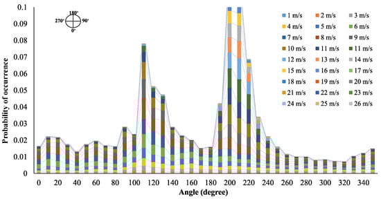
Figure 4.
Histogram of wind speed and directions.
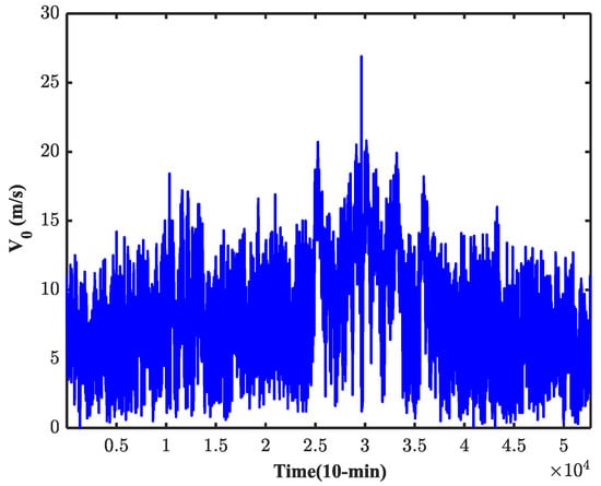
Figure 5.
Wind speed profile for a year.
To determine the PV plant size, the 10-min global horizontal irradiance (GHI) and temperature values are used to get the output power of each PV module. The GHI profile of the selected site is shown in Figure 6. This case study is simulated in Matlab following the steps of the proposed approach in sizing the HWSPS, as illustrated in Figure 7.
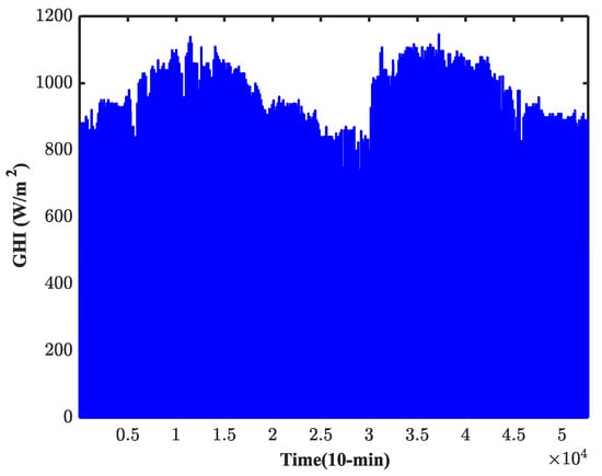
Figure 6.
Global horizontal irradiance for a year.
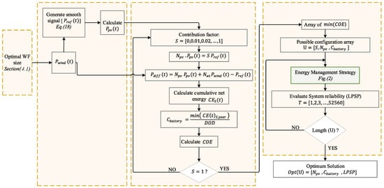
Figure 7.
Flow chart for the proposed approach of HWSPS.
7. Results and Discussion
The previous sections describe the approach to size the HWSPS. The approach was divided into two main stages. The first stage is to get the optimal wind farm layout, taking the wake effect model into consideration. The second stage is to get an optimal size of PV and BESS based on the smoothed output of wind power. The results yielded from the simulation are presented in the following subsections.
7.1. Wind Farm Size
To make the optimization as close to the real situation as possible, multi-speed and multi-direction wind profiles are engaged. In this stage, the wind histogram is used instead of each of the 10-min inputs to reduce the computational time. Running the optimization problem stated in Section 4.1 using GA yields a wind farm with 10 turbines allocated as in Figure 8. They are allocated in the borders of the wind farm to minimize the wake effects among them. The wind farm’s layout is rotated counterclockwise with respect to the southeast direction using a passive transformation matrix. An example of the wake effect with the wind blowing from an angle of is shown in Figure 9, where , , , , , and do not have velocity deficits, but the downstream turbines are all affected by the wakes of the upstream turbines.
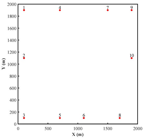
Figure 8.
Optimal wind farm layout.
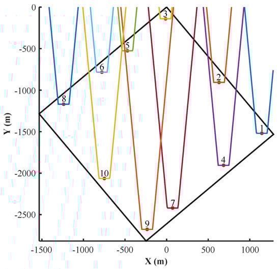
Figure 9.
Wake effects for a wind direction of .
Applying the wake effect model gives more accuracy and realistic results for a wind farm’s power generation []. The total velocity loss due to the wake effect of turbines is around 7.3% from the available wind speed. This corresponds to a loss in the wind farm’s generation power of around 11.6%.
To clarify the impact of the wake effect on wind power generation, Figure 10 shows the wind farm’s power generation with and without the wake effect using the optimal layout in Figure 8. The difference between the two scenarios is clear, and using the wake effect model supports the planners in getting more realistic wind farm generation.
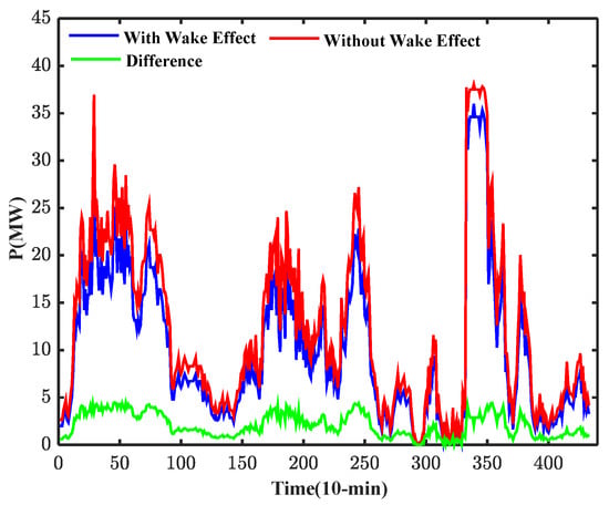
Figure 10.
The wind farm’s output power for three days.
The wake effect strongly affected the WFLO: Running the optimization problem with a zero wake effect yields a wind farm with a higher number of turbines (i.e, ), as shown in Figure 11.

Figure 11.
Optimal WFLO with a zero wake effect.
7.2. PV and BESS Sizes
The next step in the proposed approach is to generate a smooth wind output power () using MAV to reduce the fluctuations in the wind farm’s output power with the aid of a PV plant and BESS. The main purpose of smoothing the wind generation is to reduce the ramping rate, which is clearly illustrated in Figure 12 for the ramping rates at each time instant before and after smoothing. The maximum ramping before smoothing is 32.26 MW and only 3.11 MW after smoothing. This means that the maximum ramping in the is less than 8.12% of the wind farm’s capacity, which is sufficient to proceed with this case study.
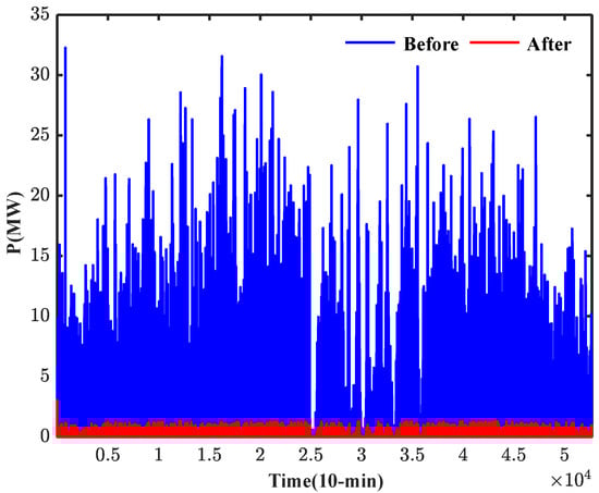
Figure 12.
The wind farm’s annual ramping rate.
Hence, the generated is used with a MAV with 30 data points, as presented in Figure 13. It is clear that is smoother than the actual . The purple bounded areas in Figure 13 show the shortages of to fulfill the . Thus, to mitigate this shortage, PV with BESS is added with 100 contribution factors , as explained in Section 4.3.
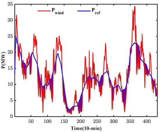
Figure 13.
Sample of actual and smoothed wind power.
Running the developed approach in NIA yields different configurations of PV and BESS with COE and LPSP, as shown in Figure 14. The BESS sizes decreased with each increment in S until S = 0.04, and then the size is fixed because the sizing of BESS is designed so as to avoid oversizing by considering only the minimum annual negative accumulative net energy (CE) using Equation (22). The minimum CE value in the whole year is 0.97708 MWh.
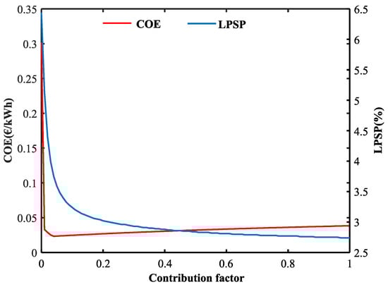
Figure 14.
COE and LPSP for different contribution factors.
The BESS capacity started from 20.56 MWh for S = 0, and then it reached 1.2213 MWh for . The minimum COE is 0.0233 €/kWh with 1.2213 MWh and 14.501 MW for the BESS and PV sizes, respectively. A summary of the optimum results is shown in Table 1.

Table 1.
Optimal HWSPS configurations from the proposed approach.
As shown in Figure 15, there is still a shortage to fulfill the reference power, but the whole LPSP represents only 3.75% during the year, with the most deficit happening during the nighttime in the absence of PV generation. The size of PV increases linearly with an increase in a contribution factor , which leads to higher fluctuations and more damped power. The deficit power decreases with an increase in a contribution factor, but the COE increases too. At the same time, BESS SOC highly fluctuates between and for charging and discharging conditions. During the daytime, there is sufficient to mitigate the shortage of wind generation. Part of the excess energy is used to charge the BESS. The BESS charged and discharged mostly during the nighttime and at the beginning and end of the daytime, as presented in Figure 16.
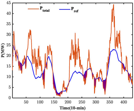
Figure 15.
Sample of total output power and smoothed wind power.
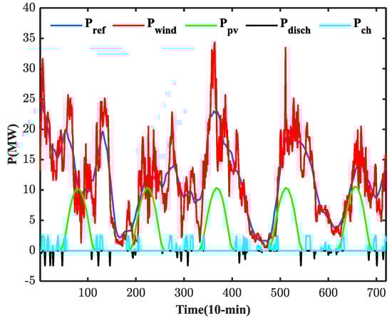
Figure 16.
Sample of 5-day HWSPS output power profiles.
7.3. Sensitivity Analysis
Further analysis is conducted to evaluate the influences of the wake effect, contribution factor, and wind generation in the developed approach. All these factors have significant impacts on the sizing of the HWSPS as presented in the following subsections.
7.3.1. Sizing without the Wake Effect
As per the aforementioned explanation about the wake effects in the wind farm, a simulation is carried out to get optimal HWSPS without considering the wake effect. The simulation ran at the optimal contribution factor (i.e., ). This yields an HWSPS with a 16.67-MW PV plant and a 1.466-MWh BESS with a COE of 0.0239 €/kWh. The COE and the sizes of PV and BESS increased by 2.58%, 14.95%, and 20%, respectively. The LPSP has improved by 3.65%, which is better than when the wake effect is considered. However, this value of LPSP could be reached if the wake effect is considered with a COE of 0.0235 €/kWh when S = 0.05, with a 1.2213-MWh BESS capacity and an 18.126-MW PV plant size. This discloses the overestimation that occurred in defining the HWSPS size if the wake effect is not considered.
7.3.2. Effect of the Contribution Factor on the Sizes of PV and BESS
The cost of the wind farm alone is lower than the optimum cost of the proposed HWPS. However, the LPSP of HWSPS is 3.75%, compared to 7.84% for a stand-alone wind farm, which means that the reliability of the system improved by around 4.09% for HWSPS. This is an indicator that the wind farm alone cannot fulfill the system’s reliability. Increasing the sizes of PV and BESS leads to an improvement in LLP, but, on the other side, the COE increases. In addition, the excess power also increased, leading to a reduction in revenues. In the meantime, the fluctuation rate increases from 1.3 to 136 for and , respectively. Thus, the availability of other resources within the wind farm has a positive impact on the electrical system but only until a certain level of resource penetration.
7.3.3. Effect of Wind Power on Sizing HWSPS
To evaluate the impact of the wind power on the developed approach for sizing HWSPS, the value of each time changed by ± 20% with steps of ± 5%. The sizes of PV and BESS with COE in each scenario are shown in Table 2. The results show the impact of wind power on the COE and the sizes of PV and BESS. The COE increased by 4.29% if the wind power was curtailed by 20%. On the other hand, the COE decreased by 3% with an increment in of 20%
Table 2.
Effect of wind power on the sizes of PV and BESS.
8. Conclusions
In this paper, an approach is developed to get an optimal HWSPS using GA-NIA. The approach is sizing the PV and BESS based on the wind farm’s output. Compared with previous studies, this approach did not take the load profile into account for sizing the HWSPS. It takes the MAV of wind power as a reference to determine the optimal size of HWSPS. In addition, the GA is used in the first stage of the approach, taking Jensen’s wake effect model into consideration to get more accurate and reasonable results. The study focused on sizing the HWSPS in a way to reduce the wind farm’s output fluctuations to enhance its reliability. The sizing of PV and BESS is a matter of trade-off between system cost and reliability using the NIA.
The proposed approach is demonstrated at a site in the Sultanate of Oman using real GHI data with a multi-speed and multi-directional wind profile. The wake effect of turbines is illustrated for the selected site, and a comparison was made between the wind farm’s power generation with and without the wake effect model. The optimal HWSPS resulted in a 2.64:1 ratio of wind to PV combination. Furthermore, the corresponding BESS capacity represents 2.3% of HWSPS’s rating. In addition, a sensitivity analysis is conducted to evaluate the influences of the wake effect, contribution factor, and wind generation on the sizing of the HWSPS. This analysis reveals the importance of the wake effect to avoid overestimating the HWSPS size.
Thus, the overall developed approach is adequate and effective in performing a feasibility study for the sizing of HWSPS with minimum costs of energy. As a future study, it is worth investigating the developed approach using other renewable resources to get a cost-effective and reliable system. In addition, this research could be extended by considering other wake effect models and smoothing techniques.
Author Contributions
Conceptualization, A.A.S.; Methodology, A.A.S.; Software, A.A.S.; Validation, A.A.-H., M.A. and R.A.-A.; Investigation, M.A.; Resources, A.A.-H.; Writing—original draft preparation, A.A.S.; Supervision, A.A.-H.; Writing—review and editing, A.A.-H. and R.A.-A. All authors have read and agreed to the published version of the manuscript.
Funding
This research is partially supported by His Majesty Trust Fund awarded to Sultan Qaboos University research team (SR/ENG/ECED/17/01).
Acknowledgments
The authors would like to thank Sultan Qaboos University, Oman Rural Areas Electricity Company (RAEC), HMTF project code (SR/ENG/ECE/17/01), Baraa and Mostafa for their guidance and support to this research work.
Conflicts of Interest
The authors declare no conflict of interest.
Nomenclatures
| free stream wind speed (m/s) | |
| wind speed at position n (m/s) | |
| wind direction angle (∘) | |
| x-coordinate of turbine i (m) | |
| x-coordinate of turbine n (m) | |
| wind turbine hub height (m) | |
| downstream rotor radius of turbine n (m) | |
| upstream rotor radius of turbine i (m) | |
| wake radius in turbine n due to turbine i (m) | |
| y-coordinate of turbine i (m) | |
| y-coordinate of turbine n (m) | |
| horizontal distance between turbines i and n (m) | |
| perpendicular distance between turbines i and n (m) | |
| capital cost of the wind turbine (€) | |
| capital cost of the PV module (€) | |
| capital cost of the battery (€) | |
| capital cost of inverter (€) | |
| lifetime of the project (year) | |
| lifetime of the unit (year) | |
| number of batteries (Nos.) | |
| number of inverters (Nos.) | |
| wind generation (MW) | |
| solar generation (MW) | |
| smoothed reference power (MW) | |
| C | battery C-rate |
| battery charge energy (MWh) | |
| battery discharge energy (MWh) | |
| wind energy (MWh) | |
| solar energy (MWh) | |
| number of PV modules (Nos.) | |
| number of wind turbines (Nos.) | |
| battery charge power (MW) | |
| battery discharge power (MW) | |
| cumulative net energy (MWh) | |
| battery capacity (MWh) |
Appendix A
Specifications of the used wind turbine, PV module, BESS, and inverter:
| Wind Turbine | PV | ||
| Rated power | 3.83 MW | Model | Polycrystalline |
| Hub Height | 80 m | Maximum power at | 275 W |
| Rotor diameter | 130 m | Temperature coefficient of | −0.47 |
| Capital cost | 1784 €/kW | Capital cost | 598.62 €/kW |
| O&M cost | 3% capital cost/year | O&M cost | 1 % capital cost/year |
| Lifetime | 20 years | Lifetime | 20 years |
| BESS | Inverter | ||
| Nominal Capacity | 1000 Ah | Rated Power | 115 kW |
| Nominal Voltage | 2 V | efficiency () | 90% |
| Capital cost | 213 €/kWh | Capital cost | 117.26 €/kW |
| Replacement cost | 213 €/kWh | Replacement cost | 117.26 €/kW |
| O&M cost | 9.8 €/year | O&M cost | 0.92 €/kW/year |
| Lifetime | 5 years | Lifetime | 20 years |
References
- Khalid, M.; Ahmadi, A.; Savkin, A.V.; Agelidis, V.G. Minimizing the energy cost for microgrids integrated with renewable energy resources and conventional generation using controlled battery energy storage. Renew. Energy 2016, 97, 646–655. [Google Scholar] [CrossRef]
- Mahesh, A.; Sandhu, K.S. Hybrid wind/photovoltaic energy system developments: Critical review and findings. Renew. Sustain. Energy Rev. 2015, 52, 1135–1147. [Google Scholar] [CrossRef]
- Luna-Rubio, R.; Trejo-Perea, M.; Vargas-Vázquez, D.; Ríos-Moreno, G. Optimal sizing of renewable hybrids energy systems: A review of methodologies. Sol. Energy 2012, 86, 1077–1088. [Google Scholar] [CrossRef]
- Jakhrani, A.Q.; Othman, A.K.; Rigit, A.R.H.; Samo, S.R.; Kamboh, S.A. A novel analytical model for optimal sizing of standalone photovoltaic systems. Energy 2012, 46, 675–682. [Google Scholar] [CrossRef]
- Alsadi, S.; Khatib, T. Photovoltaic power systems optimization research status: A review of criteria, constrains, models, techniques, and software tools. Appl. Sci. 2018, 8, 1761. [Google Scholar] [CrossRef]
- Upadhyay, S.; Sharma, M. A review on configurations, control and sizing methodologies of hybrid energy systems. Renew. Sustain. Energy Rev. 2014, 38, 47–63. [Google Scholar] [CrossRef]
- Al Busaidi, A.S.; Kazem, H.A.; Al-Badi, A.H.; Khan, M.F. A review of optimum sizing of hybrid PV–Wind renewable energy systems in oman. Renew. Sustain. Energy Rev. 2016, 53, 185–193. [Google Scholar] [CrossRef]
- Rajkumar, R.; Ramachandaramurthy, V.K.; Yong, B.; Chia, D. Techno-economical optimization of hybrid pv/wind/battery system using Neuro-Fuzzy. Energy 2011, 36, 5148–5153. [Google Scholar] [CrossRef]
- Ghorbani, N.; Kasaeian, A.; Toopshekan, A.; Bahrami, L.; Maghami, A. Optimizing a hybrid wind-PV-battery system using GA-PSO and MOPSO for reducing cost and increasing reliability. Energy 2018, 154, 581–591. [Google Scholar] [CrossRef]
- Bilal, B.O.; Sambou, V.; Ndiaye, P.; Kébé, C.; Ndongo, M. Multi-objective design of PV-wind-batteries hybrid systems by minimizing the annualized cost system and the loss of power supply probability (LPSP). In Proceedings of the 2013 IEEE International Conference on Industrial Technology (ICIT), Cape Town, South Africa, 25–28 February 2013; IEEE: Piscataway, NJ, USA, 2013; pp. 861–868. [Google Scholar]
- Li, C.; Ge, X.; Zheng, Y.; Xu, C.; Ren, Y.; Song, C.; Yang, C. Techno-economic feasibility study of autonomous hybrid wind/PV/battery power system for a household in Urumqi, China. Energy 2013, 55, 263–272. [Google Scholar] [CrossRef]
- Song, M.; Chen, K.; Zhang, X.; Wang, J. The lazy greedy algorithm for power optimization of wind turbine positioning on complex terrain. Energy 2015, 80, 567–574. [Google Scholar] [CrossRef]
- Malheiro, A.; Castro, P.M.; Lima, R.M.; Estanqueiro, A. Integrated sizing and scheduling of wind/PV/diesel/battery isolated systems. Renew. Energy 2015, 83, 646–657. [Google Scholar] [CrossRef]
- Kaabeche, A.; Belhamel, M.; Ibtiouen, R. Sizing optimization of grid-independent hybrid photovoltaic/wind power generation system. Energy 2011, 36, 1214–1222. [Google Scholar] [CrossRef]
- Abbes, D.; Martinez, A.; Champenois, G. Life cycle cost, embodied energy and loss of power supply probability for the optimal design of hybrid power systems. Math. Comput. Simul. 2014, 98, 46–62. [Google Scholar] [CrossRef]
- Akram, U.; Khalid, M.; Shafiq, S. Optimal sizing of a wind/solar/battery hybrid grid-connected microgrid system. IET Renew. Power Gener. 2017, 12, 72–80. [Google Scholar] [CrossRef]
- Howlader, A.M.; Urasaki, N.; Yona, A.; Senjyu, T.; Saber, A.Y. A review of output power smoothing methods for wind energy conversion systems. Renew. Sustain. Energy Rev. 2013, 26, 135–146. [Google Scholar] [CrossRef]
- Li, X.; Hui, D.; Lai, X. Battery energy storage station (BESS)-based smoothing control of photovoltaic (PV) and wind power generation fluctuations. IEEE Trans. Sustain. Energy 2013, 4, 464–473. [Google Scholar] [CrossRef]
- Hill, C.A.; Such, M.C.; Chen, D.; Gonzalez, J.; Grady, W.M. Battery energy storage for enabling integration of distributed solar power generation. IEEE Trans. Smart Grid 2012, 3, 850–857. [Google Scholar] [CrossRef]
- Akatsuka, M.; Hara, R.; Kita, H.; Ito, T.; Ueda, Y.; Saito, Y. Estimation of battery capacity for suppression of a PV power plant output fluctuation. In 2010 35th IEEE Photovoltaic Specialists Conference; IEEE: Piscataway, NJ, USA, 2010; pp. 000540–000543. [Google Scholar]
- Cheng, F.; Willard, S.; Hawkins, J.; Arellano, B.; Lavrova, O.; Mammoli, A. Applying battery energy storage to enhance the benefits of photovoltaics. In 2012 IEEE Energytech; IEEE: Piscataway, NJ, USA, 2012; pp. 1–5. [Google Scholar]
- Muyeen, S.; Shishido, S.; Ali, M.H.; Takahashi, R.; Murata, T.; Tamura, J. Application of energy capacitor system to wind power generation. Wind Energy Int. J. Prog. Appl. Wind Power Convers. Technol. 2008, 11, 335–350. [Google Scholar] [CrossRef]
- Kim, T.; Moon, H.j.; Kwon, D.h.; Moon, S.i. A smoothing method for wind power fluctuation using hybrid energy storage. In Proceedings of the 2015 IEEE Power and Energy Conference at Illinois (PECI), Champaign, IL, USA, 20–21 February 2015; IEEE: Piscataway, NJ, USA, 2015; pp. 1–6. [Google Scholar]
- Balamurugan, E.; Venkatasubramanian, S. Analysis of double moving average power smoothing methods for photovoltaic systems. Int. Res. J. Eng. Technol. 2016, 3, 1260–1262. [Google Scholar]
- Sukumar, S.; Mokhlis, H.; Mekhilef, S.; Karimi, M.; Raza, S. Ramp-rate control approach based on dynamic smoothing parameter to mitigate solar PV output fluctuations. Int. J. Electr. Power Energy Syst. 2018, 96, 296–305. [Google Scholar] [CrossRef]
- Sandhu, K.S.; Mahesh, A. A new approach of sizing battery energy storage system for smoothing the power fluctuations of a PV/wind hybrid system. Int. J. Energy Res. 2016, 40, 1221–1234. [Google Scholar] [CrossRef]
- Ellis, A.; Schoenwald, D.; Hawkins, J.; Willard, S.; Arellano, B. PV output smoothing with energy storage. In Proceedings of the 2012 38th IEEE Photovoltaic Specialists Conference, Austin, TX, USA, 3–8 June 2012; IEEE: Piscataway, NJ, USA, 2012; pp. 001523–001528. [Google Scholar]
- Chanhom, P.; Sirisukprasert, S.; Hatti, N. A new mitigation strategy for photovoltaic power fluctuation using the hierarchical simple moving average. In 2013 IEEE International Workshop on Inteligent Energy Systems (IWIES); IEEE: Piscataway, NJ, USA, 2013; pp. 28–33. [Google Scholar]
- Gao, X.; Yang, H.; Lu, L. Study on offshore wind power potential and wind farm optimization in Hong Kong. Appl. Energy 2014, 130, 519–531. [Google Scholar] [CrossRef]
- Appelbaum, J.; Maor, T. Dependence of PV Module Temperature on Incident Time-Dependent Solar Spectrum. Appl. Sci. 2020, 10, 914. [Google Scholar] [CrossRef]
- Dai, Q.; Liu, J.; Wei, Q. Optimal photovoltaic/battery energy storage/electric vehicle charging station design based on multi-agent particle swarm optimization algorithm. Sustainability 2019, 11, 1973. [Google Scholar] [CrossRef]
- Ma, T.; Javed, M.S. Integrated sizing of hybrid PV-wind-battery system for remote island considering the saturation of each renewable energy resource. Energy Convers. Manag. 2019, 182, 178–190. [Google Scholar] [CrossRef]
- Shajari, S.; Pour, R.K. Reduction of energy storage system for smoothing hybrid wind-PV power fluctuation. In 2012 11th International Conference on Environment and Electrical Engineering; IEEE: Piscataway, NJ, USA, 2012; pp. 115–117. [Google Scholar]
- Tao, S.; Xu, Q.; Feijóo, A.; Kuenzel, S.; Bokde, N. Integrated Wind Farm Power Curve and Power Curve Distribution Function Considering the Wake Effect and Terrain Gradient. Energies 2019, 12, 2482. [Google Scholar] [CrossRef]
- Gao, X.; Yang, H.; Lin, L.; Koo, P. Wind turbine layout optimization using multi-population genetic algorithm and a case study in Hong Kong offshore. J. Wind Eng. Ind. Aerodyn. 2015, 139, 89–99. [Google Scholar] [CrossRef]
- Mosetti, G.; Poloni, C.; Diviacco, B. Optimization of wind turbine positioning in large windfarms by means of a genetic algorithm. J. Wind Eng. Ind. Aerodyn. 1994, 51, 105–116. [Google Scholar] [CrossRef]
- Lee, D.; Kim, J.; Baldick, R. Ramp Rates Control of Wind Power Output Using a Storage System and Gaussian Processes; University of Texas at Austin, Electrical and Computer Engineering: Austin, TX, USA, 2012. [Google Scholar]
- Feng, L.; Zhang, J.; Li, G.; Zhang, B. Cost reduction of a hybrid energy storage system considering correlation between wind and PV power. Prot. Control Mod. Power Syst. 2016, 1, 11. [Google Scholar] [CrossRef]
- Lam, R.K.; Yeh, H.G. PV ramp limiting controls with adaptive smoothing filter through a battery energy storage system. In Proceedings of the 2014 IEEE Green Energy and Systems Conference (IGESC), Long Beach, CA, USA, 24 November 2014; IEEE: Piscataway, NJ, USA, 2014; pp. 55–60. [Google Scholar]
- Lee, H.J.; Choi, J.Y.; Park, G.S.; Oh, K.S.; Won, D.J. Renewable integration algorithm to compensate PV power using battery energy storage system. In Proceedings of the 2017 6th International Youth Conference on Energy (IYCE), Budapest, Hungary, 21–24 June 2017; IEEE: Piscataway, NJ, USA, 2017; pp. 1–6. [Google Scholar]
- Hatata, A.; Osman, G.; Aladl, M. An optimization method for sizing a solar/wind/battery hybrid power system based on the artificial immune system. Sustain. Energy Technol. Assess. 2018, 27, 83–93. [Google Scholar] [CrossRef]
- Fathima, A.; Palanisamy, K.; Padmanaban, S.; Subramaniam, U. Intelligence-based battery management and economic analysis of an optimized dual-Vanadium Redox Battery (VRB) for a Wind-PV HYBRID SYSTEM. Energies 2018, 11, 2785. [Google Scholar] [CrossRef]
- Xu, L.; Ruan, X.; Mao, C.; Zhang, B.; Luo, Y. An improved optimal sizing method for wind-solar-battery hybrid power system. IEEE Trans. Sustain. Energy 2013, 4, 774–785. [Google Scholar]
- Tao, S.; Kuenzel, S.; Xu, Q.; Chen, Z. Optimal Micro-Siting of Wind Turbines in an Offshore Wind Farm Using Frandsen–Gaussian Wake Model. IEEE Trans. Power Syst. 2019, 34, 4944–4954. [Google Scholar] [CrossRef]
© 2020 by the authors. Licensee MDPI, Basel, Switzerland. This article is an open access article distributed under the terms and conditions of the Creative Commons Attribution (CC BY) license (http://creativecommons.org/licenses/by/4.0/).