Modeling Framework Simulating the TERRE Activation Optimization Function

Abstract

The Trans-European Replacement Reserve Exchange (TERRE) project is the European implementation project for exchanging Balancing Energy (BE) from Replacement Reserves (RR). Its main objective is to operate a common European platform that gathers all RR Balancing Energy Orders (BEOs) from Transmission System Operators’ (TSOs) local BE markets into a Common Merit Order List (CMOL). It provides an optimized allocation of RR, covering all TSOs’ RR BE needs, by executing the Activation Optimization Function (AOF). In this paper, the mathematical formulation of the AOF is presented, which explicitly incorporates all standard products and constraints that are provisioned in the approved implementation framework. The clearing problem is formulated as a Mixed Integer Linear Programming model and solved within an iterative algorithm for the handling of Paradoxically Accepted Orders (PAOs). The modeling framework allows the coordination of two distinct market setups, i.e., the self-dispatch and central dispatch. To this end, a BEO conversion pre-process is executed for markets applying the central-dispatch setup, in order to attain the BE quantities for inclusion in the CMOL. The proposed model is evaluated using a test case including six countries that participate in the TERRE project (Portugal, Spain, France, Great Britain, Switzerland, Italy) as well as Greece.

1. Introduction

General Framework on Electricity Balancing

The integration (coupling) of European national electricity markets at all market timeframes (day-ahead, intra-day and balancing) constitutes the ultimate goal of the European Commission towards creating the “Internal Energy Market” (IEM) [1]. The core consequence of this newly-established market regime is that electricity demand is met securely at the European level by the most economic resources (generating units, demand response, energy storage systems), resulting in an increase of the overall social welfare. To be more precise, while the harmonization of wholesale prices across Europe would increase prices for some and decrease prices for others, the ability to access the cheapest resources would increase social welfare through an overall convergence in energy prices. Estimates [2,3] suggest that the potential increase in social welfare could be in the range of €16 billion to €43 billion on an annual basis by 2030. So far, a significant progress concerning the level of market integration has been achieved at the day-ahead and intra-day timeframes with the establishment of the pan-European single day-ahead coupling and single intra-day coupling, respectively [4]. On the other hand, the process of integrating the national balancing energy markets is at a primary stage of design and implementation, but major milestones have been reached towards this direction [5]. The delay in the implementation can be attributed to the underlying variations in the operation of the existing national balancing energy markets, acting as an important obstacle against the integration of the electricity markets as a whole [6,7,8,9]. Apparently, the successful completion of this final step of market harmonization is deemed necessary for the fulfilment of European Commission’s ambitions.

From a regulatory point of view, the integration and the functioning of balancing energy markets in Europe is technically and operationally governed by the provisions and the detailed rules laid down in the “Commission Regulation (EU) 2017/2195 of 23 November 2017 establishing a guideline on electricity balancing (EBGL)” [10]. In particular, EBGL provides a solid framework of the European balancing energy market target model, explains the main concepts and processes related to balancing energy markets, and defines the relevant tasks and timelines for the development of the respective European platforms to be used for the exchange of balancing energy products.

To comply with the objectives and the requirements of the aforementioned regulation, several cooperation pilot projects have been initiated across Europe. First, the Frequency Containment Reserves (FCR) cooperation project [11] is a regional project involving ten Transmission System Operators (TSOs) from seven countries (Austria (APG), Belgium (Elia), Switzerland (Swissgrid), Germany (50Hertz, Amprion, TenneT DE, TransnetBW), Western Denmark (Energinet), France (RTE), and the Netherlands (TenneT NL)). This project is based on a TSO–TSO settlement model (a model for the exchange of balancing services where the BSP provides balancing services to its connecting TSO, which then provides these services to the requesting TSO), and the FCR is procured through a Common Merit Order List (CMOL; auctions) where all TSOs forward the Balancing Energy Orders (BEOs) they receive from the Balancing Service Providers (BSPs) within their respective areas of responsibility.

Second, the International Grid Control Cooperation (IGCC) project [12] is a project targeting to increase the efficiency of balancing on a European level by performing imbalance netting of automatic Frequency Restoration Reserves (aFRR) between the TSOs of Germany, Denmark, the Netherlands, Switzerland, Czech Republic, Belgium, Austria, France, Croatia, and Slovenia. In principle, IGCC is intended to automatically compensate for any imbalances in opposite directions experienced by TSOs, enabling them to avoid simultaneous activations of aFRR in opposite directions.

Third, the Platform for the International Coordination of Automated Frequency Restoration and Stable System Operation (PICASSO) project [13] is considered as the starting point for designing, implementing and operating a platform for aFRR. Similar to the FCR project, the procurement of aFRR is carried out through a CMOL and the respective settlement of the activated BEOs is based on the TSO–TSO model.

Fourth, the project named Manually Activated Reserves Initiative (MARI) [14] has been endorsed as a reference project to set up a common European platform for the exchange of Balancing Energy (BE) from manually-activated Frequency Restoration Reserves (mFRR). Currently, 28 TSOs are active members to this project. At a high level, the rationale is the following [15]: (1) the BSPs communicate their mFRR BEOs to their related TSO; (2) the TSOs provide the BEOs, the Cross Zonal Capacities (CZCs), and their mFRR balancing needs to the MARI platform; (3) finally, an optimization algorithm clears the auction, sets the clearing prices and provides the activated BEOs and used CZCs.

Last, the Trans European Replacement Reserves Exchange (TERRE) project [16] is the European implementation project for exchanging BE from RR. The main objective of the TERRE project is to establish and operate a common European platform capable of gathering all the RR BEOs from TSOs’ local balancing energy markets and of providing an optimized allocation of RR, covering all TSOs’ RR BE needs. The mechanism for settling the activated BE by TERRE is again the TSO–TSO model [17]. So far, the TSOs which are active partners to the TERRE project are: National Grid (Great Britain), Swissgrid (Switzerland), REE (Spain), REN (Portugal), TERNA (Italy), RTE (France), CEPS (Czech Republic), and PSE (Poland) [16].

Currently, all these platforms are being developed under the specifications provisioned in the respective implementation frameworks that have been proposed by the TSOs and approved by the National Regulatory Authorities (NRAs). The main challenges surrounding such development are (1) widening their geographical scope to enable the participation of all European TSOs and (2) aligning the underlying rules and procedures with the requirements and provisions of the EBGL [18,19].

This paper focuses on the explicit modeling (problem formulation) of the Activation Optimization Function (clearing model) of the TERRE project central platform (called “LIBRA” platform) to be used for the clearing of the respective RR auctions. To the best of the authors’ knowledge, so far, there is no published work in the literature presenting such explicit modeling. Given that, this paper attempts to provide such modelling framework for the first time (main contribution), simulating appropriately all functionalities described in the official documents containing the theoretical background. However, the authors are not in a position to verify if it is an exact replication of the official algorithm in terms of problem constraints since the latter are not publicly available. In contrast to this gap for the LIBRA platform, there is extensive literature for the modeling of the European day-ahead market clearing model (Euphemia) [20,21,22]. On the other hand, in a more general framework, various studies have been carried out analyzing and highlighting the potential benefits of the cross-border balancing in the European region. In particular [23] examines the benefits for the Italian power system when balancing services are being exchanged with Austria and Slovenia, and [24] assesses the economic gains of the respective Portuguese system when sharing RR with Spain and France. In the same vein, [25,26] investigate the balancing market integration in Northern European countries emphasizing the exchange of FRR, while [27] focuses on the cross-border exchanges of FCR and FRR. Finally, [28] presents the legal framework and the general process for the design of the common mFRR clearing platform, and [29] considers coupled balancing markets at European level without incorporating all format of bids and differentiating the reserve types.

In addition to these studies, the participating TSOs have already proceeded to the appropriate modifications of their balancing rules to coordinate with the requirements of TERRE [30,31]. Specifically, since 6 January 2020 the TSOs participating in TERRE project have launched the TERRE platform which serves as the starting point for the integration of the balancing energy markets [32]. At the moment, only the Czech TSO has been connected to the platform, while go-lives for the other TSOs have been scheduled [32].

With regards to Article 19 of the EBGL, in June 2018, European TSOs performing the RR process have submitted a proposal [33] for the implementation framework for the exchange of BE from RR to NRAs for approval, which contains the high-level design of the LIBRA platform, the definition of rules and functions for its governance and operation, and the roadmap towards its implementation. Thus, this proposal and its accompanying explanatory document constitute the basis for our work.

The contributions of this work with respect to the literature concerns the explicit modeling of the LIBRA platform clearing module (Activation Optimization Function) including all its specific features, namely:

(a)

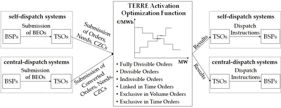
the inclusion of all formats of BEOs provisioned in the implementation framework of TERRE project and the analytical mathematical representation of their clearing conditions;

(b)

the combination of self-dispatch and central dispatch systems; for the latter, a local pre-process takes place before the TERRE clearing process for the conversion of BEOs to standard products as required by EBGL;

(c)

the implementation of imbalance netting;

(d)

the incorporation of counter-activations;

(e)

the consideration of both elastic and inelastic orders submitted by the participating TSOs so as to cover their needs, along with a tolerance band for facilitating the clearing process in the presence of large indivisible blocks; and

(f)

the inclusion of ramping constraints for the central dispatch bidding zones in the overall regional clearing model for technical feasibility purposes.

The remainder of the paper is organized as follows: Section 2 presents the conceptual framework of the RR procurement process, whereas Section 3 analyzes the format of all eligible BEOs in the LIBRA platform. Section 4 provides the detailed mathematical formulation for the clearing of the cross-zonal RR BE procurement. Section 5 elaborates on the test case and the respective results for the selected countries participating in the TERRE project (except from Poland and Czech Republic, which do not have common borders with the other countries participating in the TERRE project). Finally, the main conclusions of the conducted research are drawn in Section 6.

2. Main Balancing Arrangements Setups and RR Balancing Process

The high-level design of the LIBRA platform is schematically represented in Figure 1. There are three types of balancing market setups in terms of scheduling and dispatch arrangements (Figure 1 provides an illustrative example of these three arrangements with their specific features):

(a)

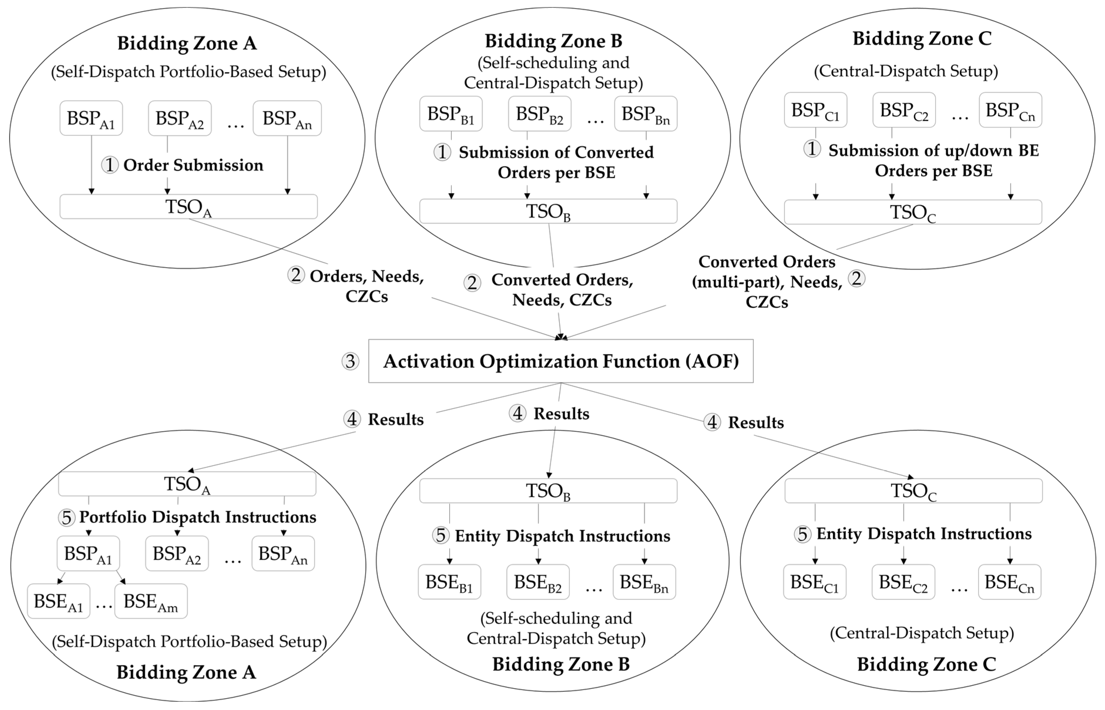
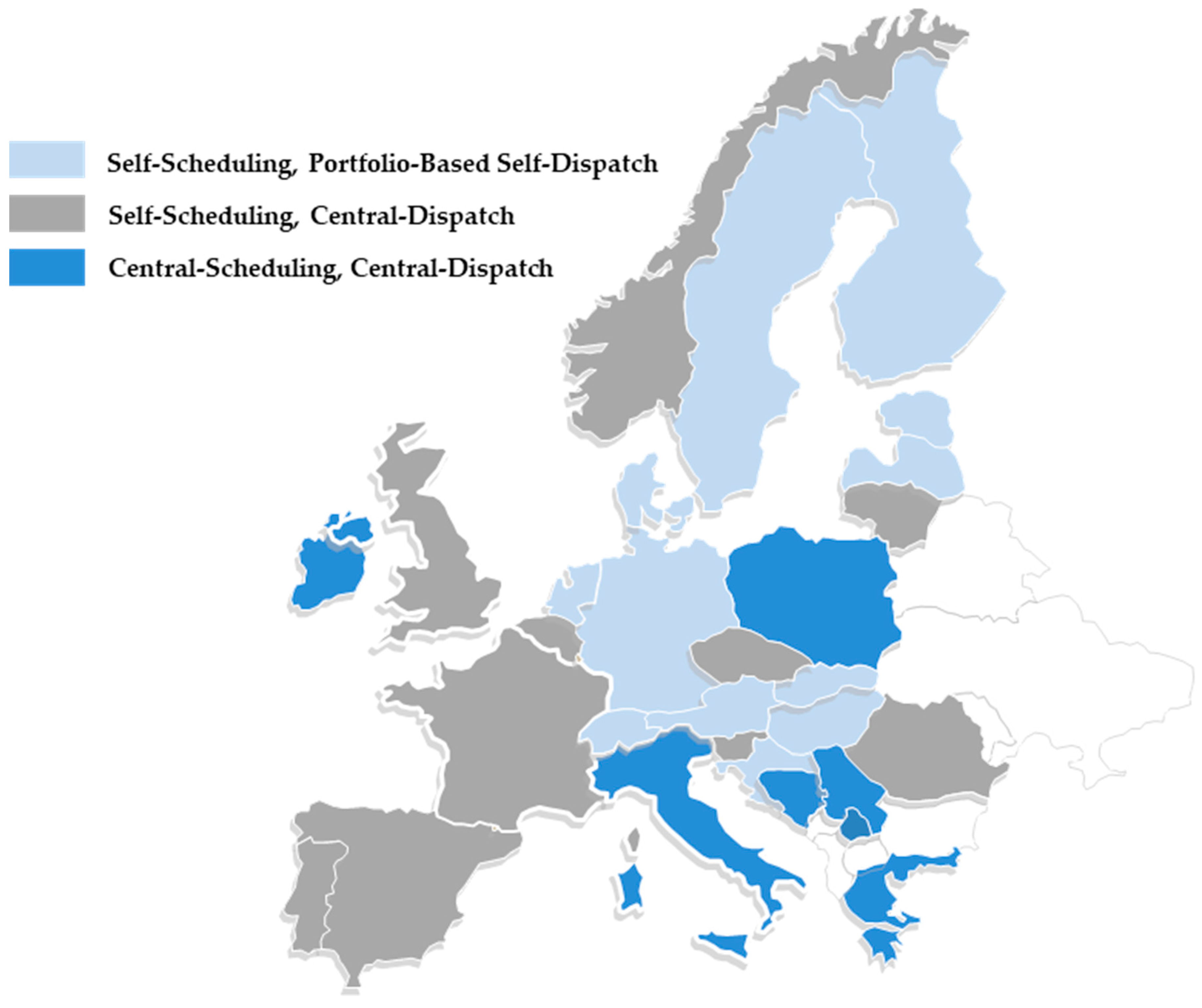
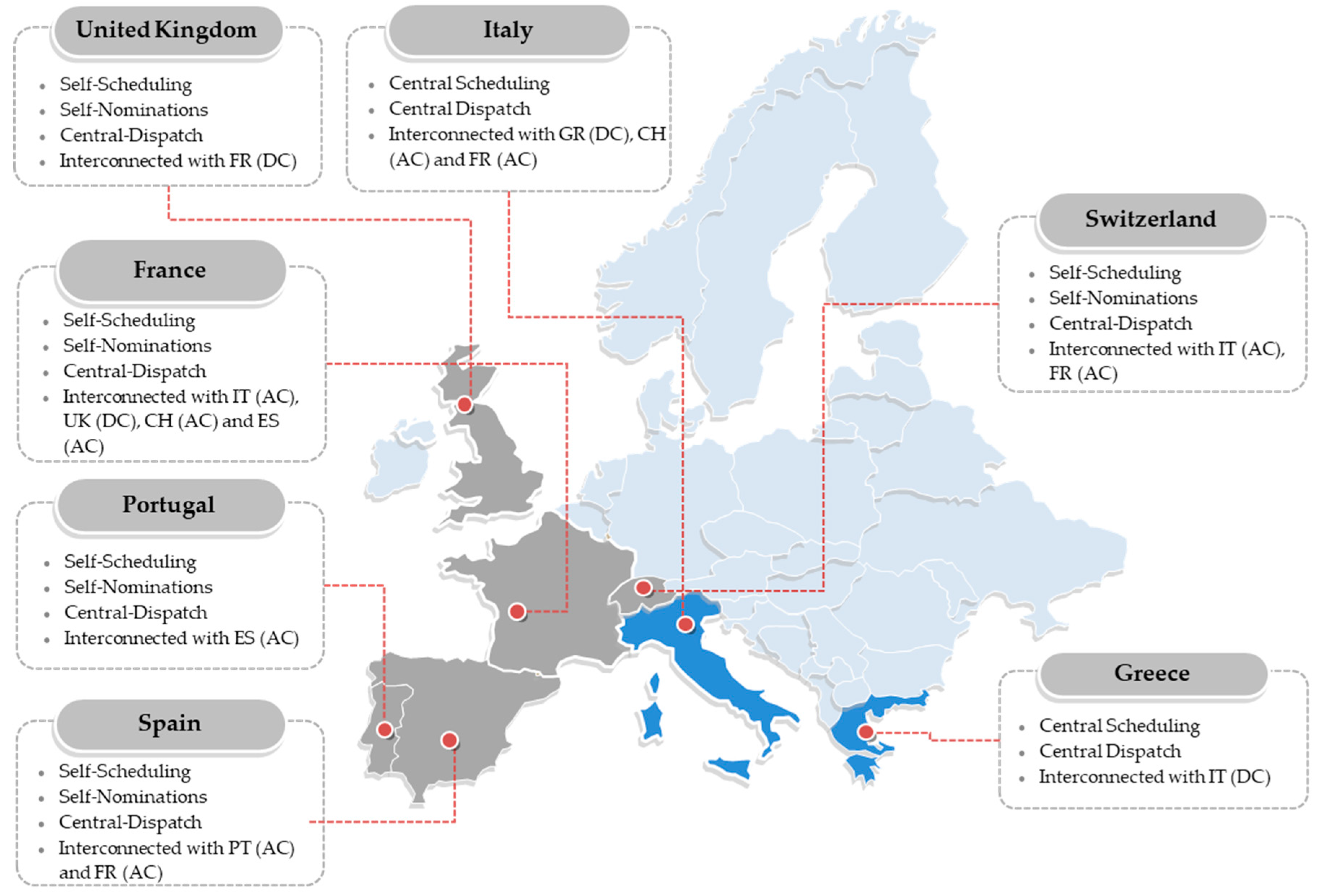
Bidding Zone A expresses the 1st setup, with self-scheduling at the day-ahead stage, issuance of portfolio-based dispatch instructions by the TSO to the BSPs and self-dispatch on an entity basis. Specifically, in this setup, the BSPs take day-ahead and/or intra-day commitment decisions for their Balance Service Entities (BSEs), namely generating units and/or demand response resources and/or energy storage resources. In real time, they acquire portfolio-based dispatch instructions by the TSO and freely allocate these instructions to their BSEs (self-scheduling), namely they determine the desired dispatch position of each BSE they operate based on their own economic criteria and taking into account BSEs’ technical constraints in conjunction with the demand elements they are balancing with. Typical examples of this setup are Switzerland, Germany, and the Netherlands, as shown in Figure 2.

(b)

Bidding Zone B expresses the 2nd setup, with self-scheduling at the day-ahead stage, participation in the real-time balancing energy market per BSE (e.g., generating unit) and central-dispatch on an entity basis (not on a portfolio basis). A typical example of this setup are France and Belgium (see Figure 2).

(c)

Bidding Zone C expresses the 3rd setup, with central (TSO-oriented) scheduling at the day-ahead stage and central (TSO-oriented) dispatch in real time on an entity basis. In this setup, the TSO considers all BSEs and the needs of the system overall to determine an efficient operational schedule (central scheduling) at the day-ahead and intra-day stage and issue optimal dispatch instructions in real time (central dispatch) directly to the BSEs. Typical examples of this setup are Italy and Greece (see Figure 2).

Taking these fundamentals into consideration, in order to participate in a coupled RR balancing energy market, BSPs from these three setups submit standard BEOs to their respective TSOs (process 1 in Figure 1). The standard formats of BEOs that can be submitted and processed by the LIBRA platform are [17]: (a) fully divisible orders (single quantity-price pair for one Real-Time Unit (RTU)) or divisible orders (similar, with a minimum quantity to be cleared) or indivisible orders (similar, with additional all-or-nothing condition); (b) linked orders in time (price-quantity pairs for successive RTUs; a same acceptance ratio “α” of the offered quantity for each linked RTU is imposed); (c) exclusive orders in volume or in time (only one of several alternative orders of a BSP in the volume or time domain is accepted); and (d) multi-part orders (stepwise orders with variable prices for variable quantities for an indicated delivery period; it allows BSPs to internally model their fixed, e.g., startup costs). The specific features of each order type are analytically described in Section 3 below.

After the BEO submission gate closure time, the TSOs anonymize and forward the submitted BEOs to the LIBRA platform (process 2 in Figure 1). In pursuant to Article 27 of EBGL, the TSOs applying the central scheduling and the central dispatch setup must convert the submitted BEOs (by the BSPs) into standard products before forwarding them to the LIBRA Platform. Here, we assume that BSPs of Bidding Zone C submit upward and downward BEOs to the TSO, and the TSO converts them into multi-part fully divisible orders. Such conversion process is deemed necessary in order to attain technically feasible dispatch instructions for the participating BSEs. Essentially, the TSO of the central-dispatch system must submit the BEOs per separate BSE, in the same format as they were initially submitted by the BSP (i.e., multi-part fully divisible orders), while also considering:

(a)

the BSEs’ technical limitations (e.g., the technical minimum, the ramp up/down rates, etc., of generating units) and

(b)

the already allocated upward and downward reserve quantities to the BSEs for FCR, aFRR, and mFRR at the formerly-executed Integrated Scheduling Process (ISP) [35]; these reserves must be available for possible activation after the RR clearing process and closer to real time (e.g., mFRR BE clearing, AGC operation, instant events).

The methodological framework and mathematical description of such conversion pre-process has been proposed in [36] and is adopted herein for the central dispatch systems. It comprises the following distinct steps:

(a)

a local RR Quantity Maximization Process, where the maximum quantity of upward and downward RR BE offered by each BSE is defined by the TSO subject to detailed unit technical limitations;

(b)

a local Mandatory Activation Process, driven by binding resource operating constraints of step (a); and

(c)

a local Conversion Process, during which the initially submitted BEOs are converted into RR standard products.

These converted BEOs are then forwarded by the respective TSO to the LIBRA platform to be included in the clearing process.

Regarding the BSPs of Bidding Zone B, we assume that they are responsible for converting their BEOs into all available order types (not only into multi-part orders, as in the case of Bidding Zone C) before sending them (per BSE) to their TSO. As far as the BSPs of Bidding Zone A are concerned, these are also responsible for submitting their BEOs in the form of standard products, however, on a portfolio basis (not per BSE).

Together with the BEOs, the TSOs also send to the platform their imbalance needs and the available CZC remaining after the latest intra-day market session (process 2 in Figure 1). The TSOs can submit inelastic (non-priced) and/or elastic (priced) orders, expressing in such way their willingness to purchase or sell BE to cover their imbalance needs. Additionally, TSOs may submit a tolerance band, their interconnection controllability constraints, the loss factors of DC interconnections, and other related data. All this data is then inserted into the platform, which executes the AOF optimizing the clearing of all TSOs’ imbalance needs against the BSPs’ submitted BEOs, using a single CMOL (process 3 in Figure 1). It is noted that the CMOL comprises two curves: a) the buying curve consisting of the positive imbalance needs (upward TSO needs/system shortage) and the downward BEOs and b) the selling curve including the negative imbalance needs (downward TSO needs/system surplus) and the upward BEOs. Figure 3 illustrates a characteristic example of these curves comprising both BSP and TSO BEOs of three bidding zones. The intersection of these two curves provides the Marginal Clearing Price (MCP) which is used for the TSO–TSO settlement process. In general, the core objective of the AOF is to maximize the social welfare (green colored area in Figure 3) of the involved parties which is defined as the area between the buying curve and the selling curve. It is important to mention that the social welfare indicated in Figure 3 corresponds to the case when no congestion occurs (adequate CZC) on the lines connecting the involved bidding zones. Instead, in cases with congested lines (inadequate CZC), the social welfare may be lower since less economical BEOs of a bidding zone shall be accepted in order to cover the desired needs.

The AOF is based on implicit auctions [37], meaning that CZC is allocated at the same time as BEOs are activated and thus the attained MCPs reflect both the congestion cost and the energy cost. Contrary to the explicit auctioning method, this capacity allocation method eliminates the cross-border trade inefficiencies and leads to maximization of the social welfare [38]. In addition, in the implicit auction method, energy always flows from a low-price bidding zone to a high-price bidding zone resulting in a price convergence between the two bidding zones (when adequate CZC is available). A last advantage of the implicit auctions is the fact that it enables bilateral cross-border trading and netting of counterflows [39]. For the purposes of the test case presented in Section 5, no bilaterals and counterflow bilaterals are taken into consideration. However, as analytically described in the same Section, a netting of the TSOs’ imbalances is inherently implemented in the model [40]. At this point, it is worth referring that the implicit capacity allocation method is currently applied in several initiatives across European power markets. The most remarkable ones are: (a) the Multi Regional Coupling (MRC) project [41] which concerns the pan-European Single Day-Ahead Coupling; (b) the 4M Market Coupling Project (Interim Coupling Project) [42] which targets to connect the borders of Czech Republic, Hungary, Romania, and Slovakia; and (c) the Cross-Border Intraday (XBID) Project [43], which constitutes the reference project for the creation of a single cross-zonal intraday market in Europe.

The results of AOF comprise the BEOs to be activated, the satisfied imbalance needs, the cross-border exchanges, and the used CZCs (process 4 in Figure 1), based on which TSOs issue dispatch instructions to the BSPs (Bidding Zone A) or directly to the BSEs (Bidding Zones B and C) in their control area (process 5 in Figure 1).

3. LIBRA Platform Orders Types

As described in [17], LIBRA platform can proceed a variety of orders types submitted by the BSPs and the respective TSOs. These formats apply both for upward and downward BEOs. In this Section, a graphical representation of the provisioned formats is provided along with a conceptual description of the core clearing conditions of each format.

Figure 4 below presents the following order types:

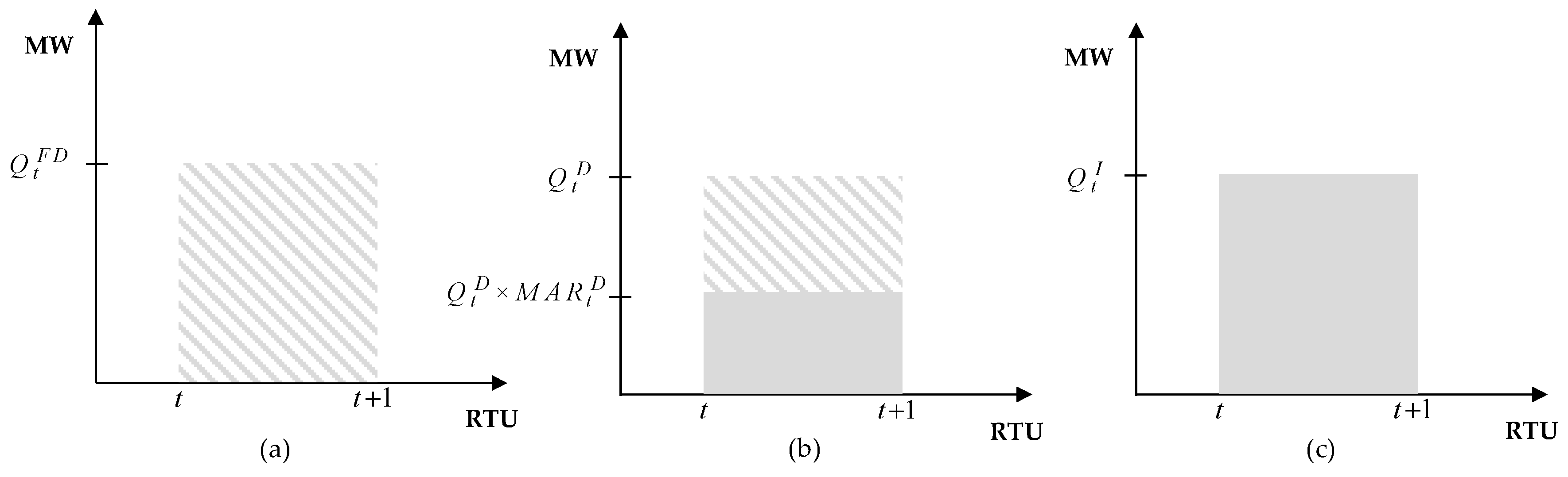
• Fully Divisible Order: It is an order submitted with a single quantity and a single price for a specific RTU. It has no minimum acceptance ratio, meaning that the quantity to be cleared by the AOF can range from zero to the offered quantity ${\mathrm{Q}}_{\mathrm{t}}^{\mathrm{F}\mathrm{D}}$ (see grey striped area in Figure 4a).
• Divisible Order: It is an order submitted with a single quantity and a single price for a specific RTU. It has a minimum acceptance ratio, meaning that the quantity to be cleared can range from a minimum quantity ${\mathrm{Q}}_{\mathrm{t}}^{\mathrm{D}}\times \mathrm{M}\mathrm{A}{\mathrm{R}}_{\mathrm{t}}^{\mathrm{D}}$ to the offered quantity ${\mathrm{Q}}_{\mathrm{t}}^{\mathrm{D}}$ (see grey striped area in Figure 4b).
• Indivisible Order: It is an order submitted with a single quantity and a single price for a specific RTU. Its minimum acceptance ratio is equal to one, meaning that the quantity to be cleared shall be identical with the offered quantity ${\mathrm{Q}}_{\mathrm{t}}^{\mathrm{I}}$ (see grey area in Figure 4c).

Another set of order types is the following:

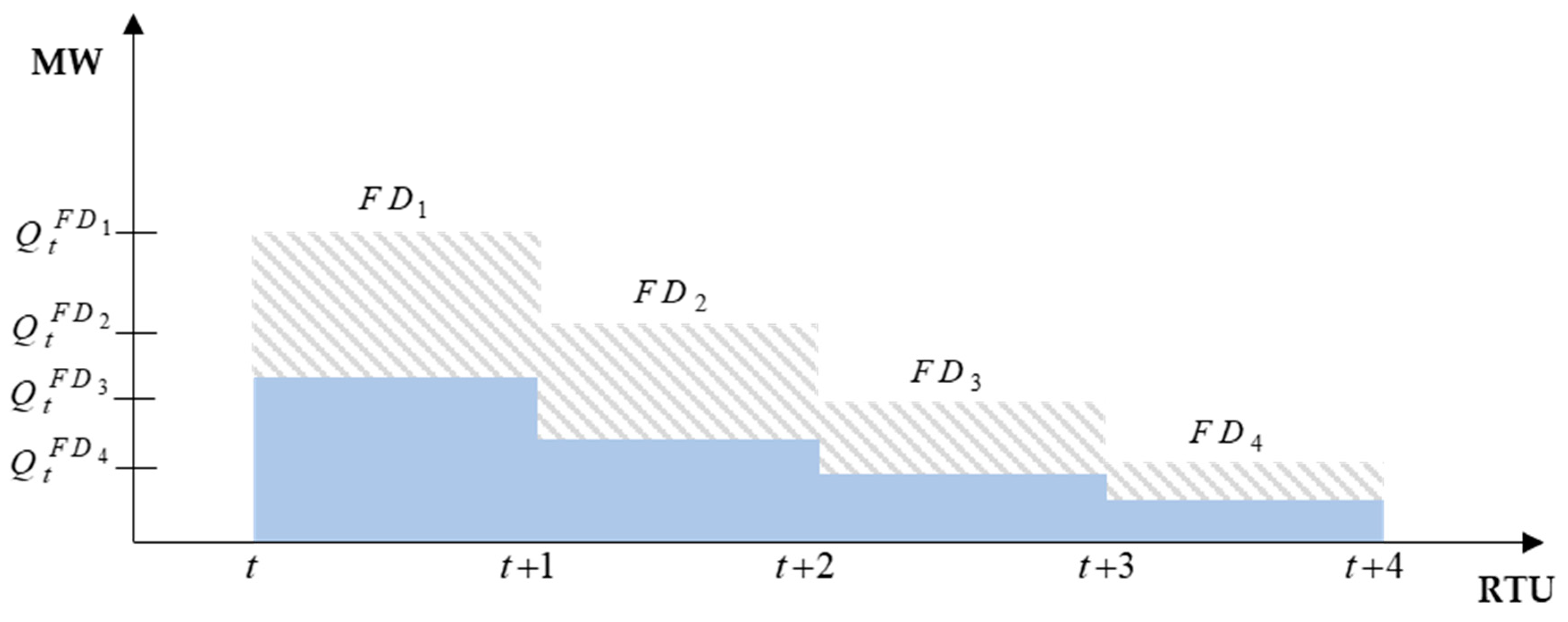
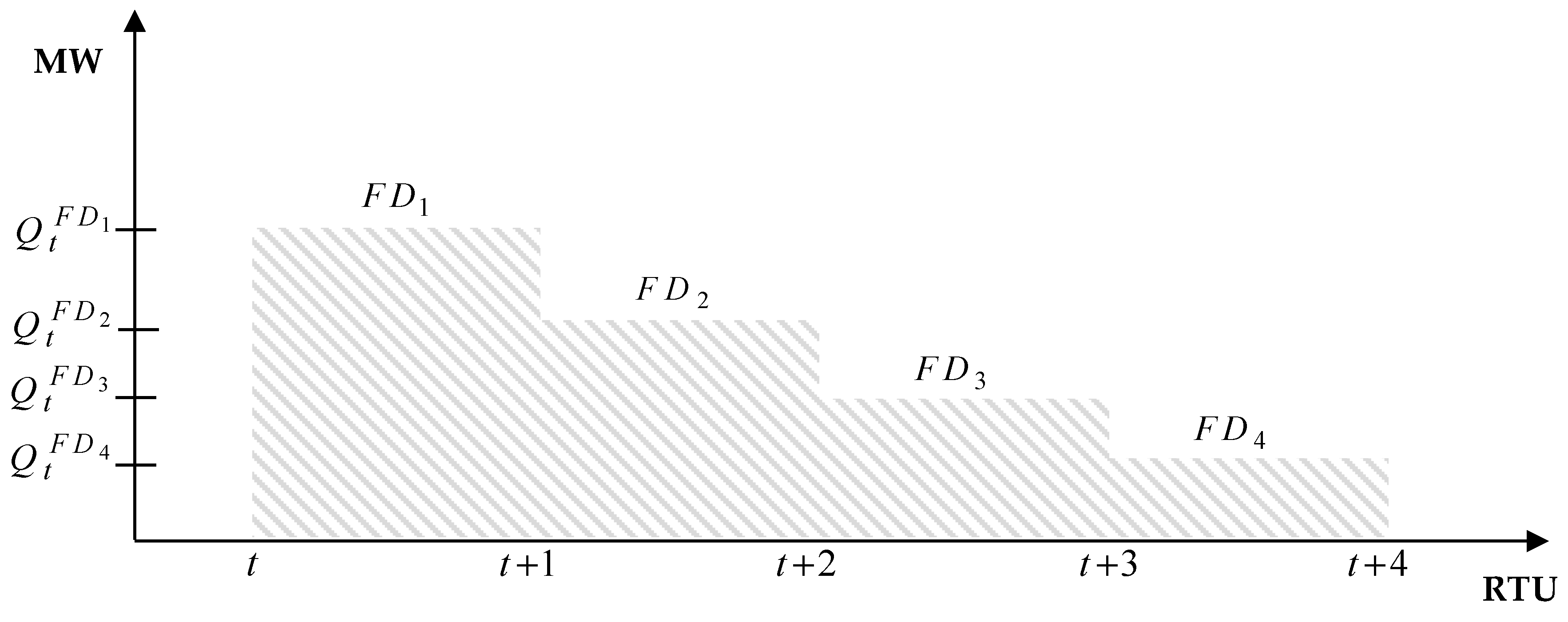
• Linked in Time Fully Divisible Orders: Discrete fully divisible orders with a single quantity and a single price which correspond to different RTUs. They have no minimum acceptance ratio. However, the attained acceptance ratios of these discrete orders shall be equal. For example, in Figure 5, four discrete fully divisible orders are presented for which the same acceptance ratio apply (see blue area).
• Linked in Time Divisible Orders: They are discrete divisible orders with a single quantity and a single price which correspond to different RTUs. They have a minimum acceptance ratio. Again, the attained acceptance ratio of these discrete orders shall be equal and greater than the minimum acceptance ratio.
• Linked in Time Indivisible Orders: They are discrete indivisible orders with a single quantity and a single price which correspond to different RTUs. Their minimum acceptance ratio is equal to one. The additional constraint is that the acceptance ratios of these discrete orders shall be equal.

For illustration purposes, a linked in time fully divisible order is presented in Figure 5 below.

The next set of order types comprises the following:

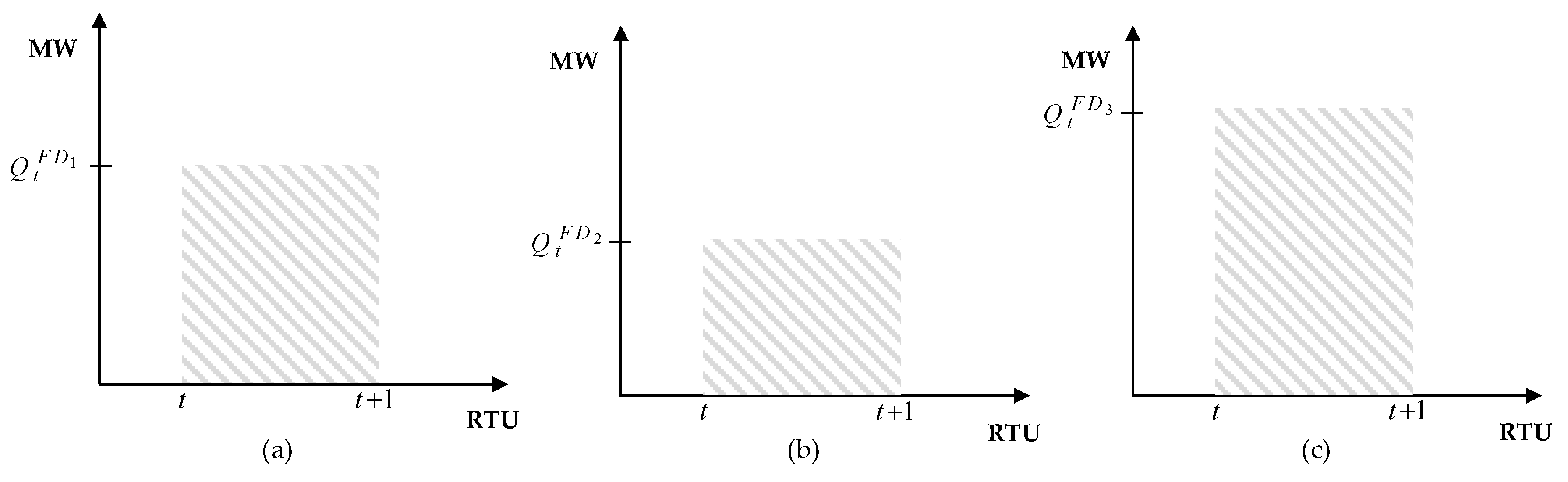
• Exclusive in Volume Fully Divisible Orders: Discrete fully divisible orders belonging to the same group, with a single quantity and a single price which correspond to the same RTU, without a minimum acceptance ratio. The additional constraint is that only one of these orders can be cleared by the AOF. For example, Figure 6 presents three discrete fully divisible orders (Figure 6a–c) corresponding to a specific RTU, where only one of them can be cleared.
• Exclusive in Volume Divisible Orders: Discrete divisible orders belonging to the same group, with a single quantity and a single price which correspond to the same RTU, with a minimum acceptance ratio. Again, only one of these orders can be cleared by the AOF.
• Exclusive in Volume Indivisible Orders: Discrete indivisible orders belonging to the same group, with a single quantity and a single price which correspond to the same RTU, with a minimum acceptance ratio equal to one. Only one of these orders can be cleared by the AOF.

The next set of order types comprises the following:

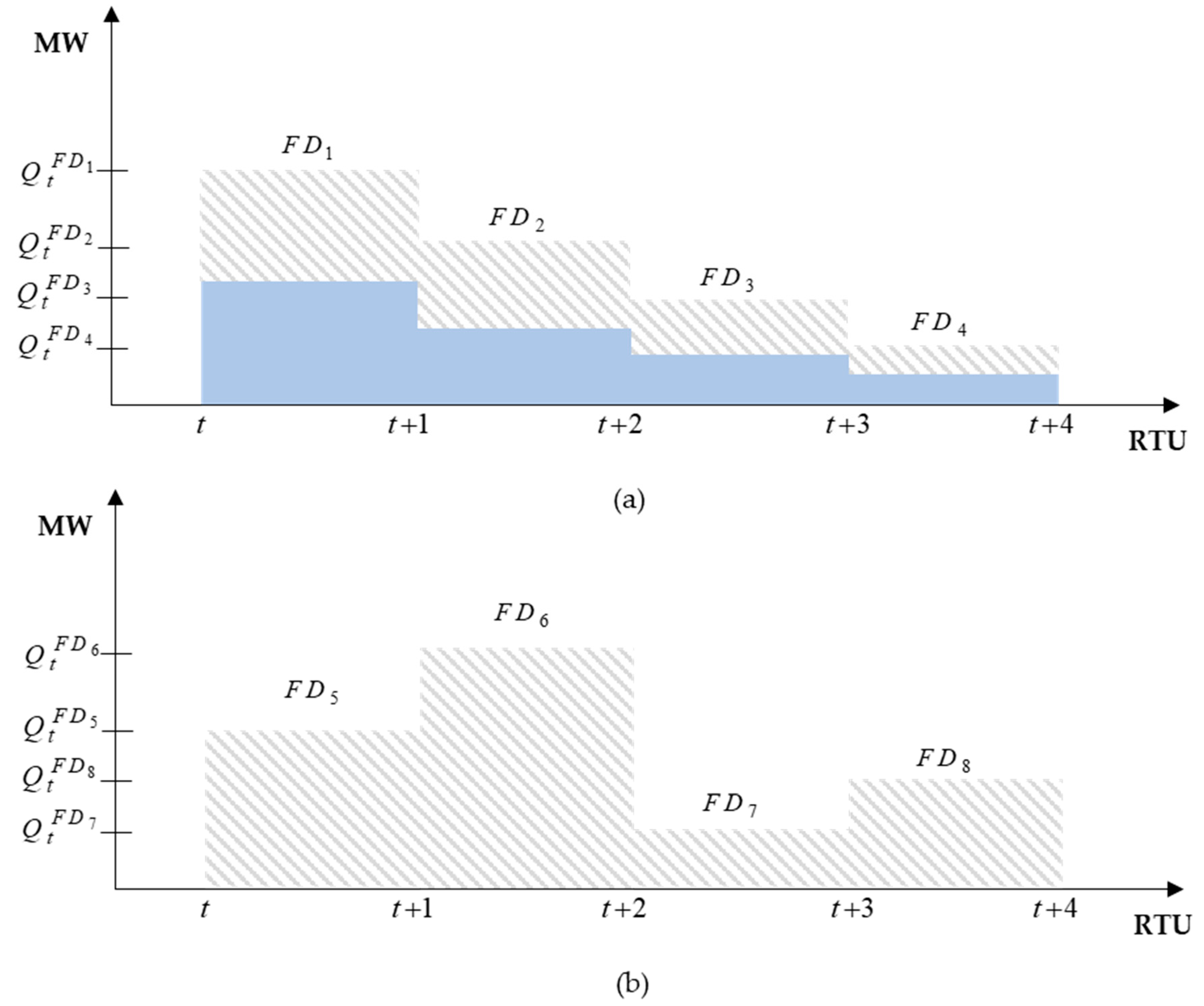
• Exclusive in Volume Linked in Time Fully Divisible Orders: Discrete fully divisible orders belonging to the same group, with a single quantity and a single price which correspond to the same RTU, without a minimum acceptance ratio. The additional constraint is that only one of these orders can be cleared by the AOF and the acceptance ratios of the cleared orders shall be equal. For example, Figure 7 presents two linked in time fully divisible orders (Figure 7a,b) belonging to the same group; only one of these two orders shall be cleared (see blue colored area in Figure 7a) and for the cleared order the same acceptance ratio shall apply for all RTUs.
• Exclusive in Volume Linked in Time Divisible Orders: Discrete divisible orders belonging to the same group, with a single quantity and a single price which correspond to the same RTU, with a minimum acceptance ratio. Again, only one of these orders can be cleared by the AOF; the acceptance ratio of the cleared orders shall be equal or greater than the minimum acceptance ratio.
• Exclusive in Volume Linked in Time Indivisible Orders: Discrete indivisible orders belonging to the same group, with a single quantity and a single price which correspond to the same RTU, with a minimum acceptance ratio equal to one. Only one of these orders can be cleared by the AOF; the acceptance ratios of the cleared orders shall be equal.

Another set of order types comprises the following:

• Exclusive in Time Fully Divisible Orders: Discrete fully divisible orders with a single quantity and a single price which correspond to different RTUs, without a minimum acceptance ratio. Only one of these orders can be cleared by the AOF. For example, in Figure 8, four discrete fully divisible orders are presented, where only one them can be cleared.
• Exclusive in Time Divisible Orders: Discrete divisible orders with a single quantity and a single price which correspond to different RTUs, with a minimum acceptance ratio. Only one of these orders can be cleared by the AOF.
• Exclusive in Time Indivisible Orders: Discrete indivisible orders with a single quantity and a single price which correspond to different RTUs, with a minimum acceptance ratio equal to one. Again, only one of these orders can be cleared by the AOF.

The last set of order types is as follows:

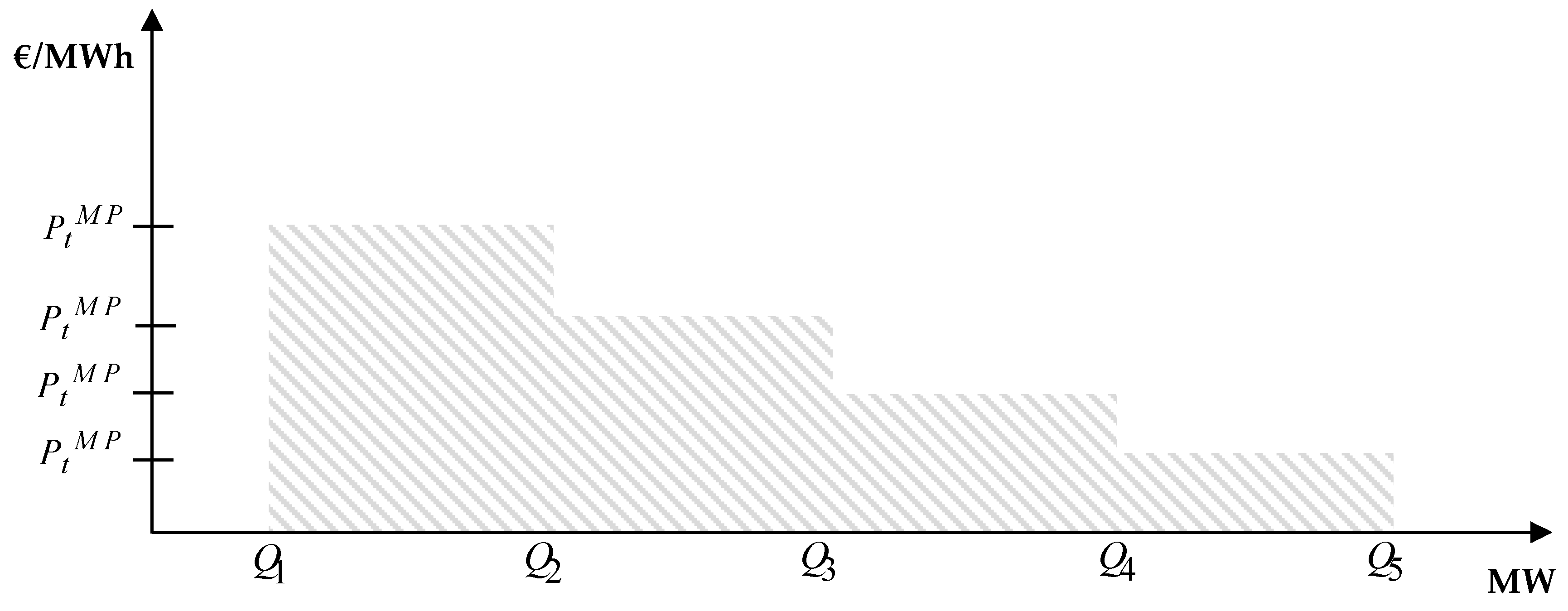
• Multi-part Fully Divisible Order: Order submitted with variable quantities and variable prices for one or more RTUs, without a minimum acceptance ratio. An example is provided in Figure 9.
• Multi-part Divisible Order: Order with variable quantities and variable prices for one or more RTUs, with a minimum acceptance ratio.
• Multi-part Indivisible Order: Order submitted with variable quantities and variable prices for one or more RTUs, with a minimum acceptance ratio equal to one.

4. Activation Optimization Function Mathematical Formulation

4.1. Problem Formulation

This Section provides the mathematical formulation that attains the goals and the required functionality of the AOF of LIBRA platform, considering the specific features of the tradable order types (described in Section 3) and the targets of the respective TSOs.

4.1.1. Objective Function

In principle, the conventional functionality of the AOF is the maximization of the overall social welfare, by clearing the buying curve (demand) against the selling curve (supply). It is noted that the positive imbalance needs (upward TSO needs/system shortage) and the downward BEOs represent the buying curve, whereas the negative imbalance needs (downward TSO needs/system surplus) and the upward BEOs represent the selling curve.

As described in Section 3, the submitted BEOs may have different delivery periods and formats. The decision about which BEOs will be activated is based upon which BEOs maximize the overall social welfare within the scheduling period. The latter is equal to one hour and comprises four (4) individual 15 min dispatch periods; the AOF does not maximize the welfare of each dispatch period separately but seeks to maximize the welfare of the whole scheduling period (hour).

The objective function maximizes the total welfare (TW) comprising the welfare of the upward and downward BEOs and the upward and downward TSO needs. Parameter D is set equal to 0.25 (quarter RTU).

$$\mathrm{M}\mathrm{a}\mathrm{x}\mathrm{T}\mathrm{W}=\mathrm{D}\cdot \left(\begin{array}{l}-{\displaystyle \sum _{\mathrm{o}{\mathrm{r}}_{\mathrm{B}\mathrm{S}\mathrm{P}}\in \mathrm{O}{\mathrm{R}}_{\mathrm{B}\mathrm{S}\mathrm{P}}^{\mathrm{u}\mathrm{p}}}{\displaystyle \sum _{\mathrm{t}\in \mathrm{T}}\left({\mathrm{P}}_{\mathrm{u}\mathrm{p},\mathrm{t}}^{\mathrm{o}{\mathrm{r}}_{\mathrm{B}\mathrm{S}\mathrm{P}}}\cdot {\mathrm{Q}}_{\mathrm{u}\mathrm{p},\mathrm{t}}^{\mathrm{o}{\mathrm{r}}_{\mathrm{B}\mathrm{S}\mathrm{P}}}\cdot {\mathrm{x}}_{\mathrm{u}\mathrm{p},\mathrm{t}}^{\mathrm{o}{\mathrm{r}}_{\mathrm{B}\mathrm{S}\mathrm{P}}}\right)}}-{\displaystyle \sum _{\mathrm{o}{\mathrm{r}}_{\mathrm{B}\mathrm{S}\mathrm{E}}\in \mathrm{O}{\mathrm{R}}_{\mathrm{B}\mathrm{S}\mathrm{E}}^{\mathrm{u}\mathrm{p}}}{\displaystyle \sum _{\mathrm{t}\in \mathrm{T}}{\displaystyle \sum _{\mathrm{k}\in \mathrm{K}}\left({\mathrm{P}}_{\mathrm{u}\mathrm{p},\mathrm{t},\mathrm{k}}^{\mathrm{o}{\mathrm{r}}_{\mathrm{B}\mathrm{S}\mathrm{E}}}\cdot {\mathrm{q}}_{\mathrm{u}\mathrm{p},\mathrm{t},\mathrm{k}}^{\mathrm{o}{\mathrm{r}}_{\mathrm{B}\mathrm{S}\mathrm{E}}}\right)-}}}\\ {\displaystyle \sum _{\mathrm{o}{\mathrm{r}}_{\mathrm{T}\mathrm{S}\mathrm{O}}\in \mathrm{O}{\mathrm{R}}_{\mathrm{T}\mathrm{S}\mathrm{O}}^{\mathrm{d}\mathrm{n}}}{\displaystyle \sum _{\mathrm{t}\in \mathrm{T}}\left({\mathrm{P}}_{\mathrm{d}\mathrm{n},\mathrm{t}}^{\mathrm{o}{\mathrm{r}}_{\mathrm{T}\mathrm{S}\mathrm{O}}}\cdot {\mathrm{Q}}_{\mathrm{d}\mathrm{n},\mathrm{t}}^{\mathrm{o}{\mathrm{r}}_{\mathrm{T}\mathrm{S}\mathrm{O}}}\cdot {\mathrm{n}}_{\mathrm{d}\mathrm{n},\mathrm{t}}^{\mathrm{o}{\mathrm{r}}_{\mathrm{T}\mathrm{S}\mathrm{O}}}\right)}}+{\displaystyle \sum _{\mathrm{o}{\mathrm{r}}_{\mathrm{B}\mathrm{S}\mathrm{P}}\in \mathrm{O}{\mathrm{R}}_{\mathrm{B}\mathrm{S}\mathrm{P}}^{\mathrm{d}\mathrm{n}}}{\displaystyle \sum _{\mathrm{t}\in \mathrm{T}}\left({\mathrm{P}}_{\mathrm{d}\mathrm{n},\mathrm{t}}^{\mathrm{o}{\mathrm{r}}_{\mathrm{B}\mathrm{S}\mathrm{P}}}\cdot {\mathrm{Q}}_{\mathrm{d}\mathrm{n},\mathrm{t}}^{\mathrm{o}{\mathrm{r}}_{\mathrm{B}\mathrm{S}\mathrm{P}}}\cdot {\mathrm{x}}_{\mathrm{d}\mathrm{n},\mathrm{t}}^{\mathrm{o}{\mathrm{r}}_{\mathrm{B}\mathrm{S}\mathrm{P}}}\right)}}+\\ {\displaystyle \sum _{\mathrm{o}{\mathrm{r}}_{\mathrm{B}\mathrm{S}\mathrm{E}}\in \mathrm{O}{\mathrm{R}}_{\mathrm{B}\mathrm{S}\mathrm{E}}^{\mathrm{d}\mathrm{n}}}{\displaystyle \sum _{\mathrm{t}\in \mathrm{T}}{\displaystyle \sum _{\mathrm{k}\in \mathrm{K}}\left({\mathrm{P}}_{\mathrm{d}\mathrm{n},\mathrm{t},\mathrm{k}}^{\mathrm{o}{\mathrm{r}}_{\mathrm{B}\mathrm{S}\mathrm{E}}}\cdot {\mathrm{q}}_{\mathrm{d}\mathrm{n},\mathrm{t},\mathrm{k}}^{\mathrm{o}{\mathrm{r}}_{\mathrm{B}\mathrm{S}\mathrm{E}}}\right)+{\displaystyle \sum _{\mathrm{o}{\mathrm{r}}_{\mathrm{T}\mathrm{S}\mathrm{O}}\in \mathrm{O}{\mathrm{R}}_{\mathrm{T}\mathrm{S}\mathrm{O}}^{\mathrm{u}\mathrm{p}}}{\displaystyle \sum _{\mathrm{t}\in \mathrm{T}}\left({\mathrm{P}}_{\mathrm{u}\mathrm{p},\mathrm{t}}^{\mathrm{o}{\mathrm{r}}_{\mathrm{T}\mathrm{S}\mathrm{O}}}\cdot {\mathrm{Q}}_{\mathrm{u}\mathrm{p},\mathrm{t}}^{\mathrm{o}{\mathrm{r}}_{\mathrm{T}\mathrm{S}\mathrm{O}}}\cdot {\mathrm{n}}_{\mathrm{u}\mathrm{p},\mathrm{t}}^{\mathrm{o}{\mathrm{r}}_{\mathrm{T}\mathrm{S}\mathrm{O}}}\right)}}}}}\end{array}\right)$$

(1)

4.1.2. Order Clearing Constraints

Constraints (2)–(42) model the clearing rules of all tradable order types provisioned in LIBRA platform [17]. In particular, Constraints (2)–(4) define the maximum acceptance ratio of each format of order, respectively (fully divisible, divisible and indivisible). Constraint (5) enforces the minimum acceptance ratio which is applied only in the case of divisible orders.

$${\mathrm{x}}_{\mathrm{d}\mathrm{r},\mathrm{t}}^{\mathrm{f}\mathrm{d}}\le 1\forall \mathrm{f}\mathrm{d}\in \mathrm{F}\mathrm{D},\mathrm{d}\mathrm{r}\in \mathrm{D}\mathrm{R},\mathrm{t}\in \mathrm{T}$$

(2)

$${\mathrm{x}}_{\mathrm{d}\mathrm{r},\mathrm{t}}^{\mathrm{d}}\le {\mathrm{u}}_{\mathrm{d}\mathrm{r},\mathrm{t}}^{\mathrm{d}}\forall \mathrm{d}\in \mathrm{D},\mathrm{d}\mathrm{r}\in \mathrm{D}\mathrm{R},\mathrm{t}\in \mathrm{T}$$

(3)

$${\mathrm{x}}_{\mathrm{d}\mathrm{r},\mathrm{t}}^{\mathrm{i}}={\mathrm{u}}_{\mathrm{d}\mathrm{r},\mathrm{t}}^{\mathrm{i}}\forall \mathrm{i}\in \mathrm{I},\mathrm{d}\mathrm{r}\in \mathrm{D}\mathrm{R},\mathrm{t}\in \mathrm{T}$$

(4)

$${\mathrm{x}}_{\mathrm{d}\mathrm{r},\mathrm{t}}^{\mathrm{d}}\ge \mathrm{M}\mathrm{A}{\mathrm{R}}_{\mathrm{d}\mathrm{r},\mathrm{t}}^{\mathrm{d}}\cdot {\mathrm{u}}_{\mathrm{d}\mathrm{r},\mathrm{t}}^{\mathrm{d}}\forall \mathrm{d}\in \mathrm{D},\mathrm{d}\mathrm{r}\in \mathrm{D}\mathrm{R},\mathrm{t}\in \mathrm{T}$$

(5)

Constraints (6)–(12) represent the clearing rules for the linked orders in time. These orders can be either fully divisible or divisible or indivisible (Constraints (6)–(9) resemble Constraints (2)–(5)) and they shall refer to different RTUs. Constraints (10)–(12) are used in order to achieve the same acceptance ratio for orders which are linked in time.

$${\mathrm{x}}_{\mathrm{d}\mathrm{r},\mathrm{t}}^{\mathrm{l}\mathrm{f}\mathrm{d}}\le 1\forall \mathrm{l}\mathrm{f}\mathrm{d}\in \mathrm{L}\mathrm{F}\mathrm{D},\mathrm{d}\mathrm{r}\in \mathrm{D}\mathrm{R},\mathrm{t}\in \mathrm{T}$$

(6)

$${\mathrm{x}}_{\mathrm{d}\mathrm{r},\mathrm{t}}^{\mathrm{l}\mathrm{d}}\le {\mathrm{u}}_{\mathrm{d}\mathrm{r},\mathrm{t}}^{\mathrm{l}\mathrm{d}}\forall \mathrm{l}\mathrm{d}\in \mathrm{L}\mathrm{D},\mathrm{d}\mathrm{r}\in \mathrm{D}\mathrm{R},\mathrm{t}\in \mathrm{T}$$

(7)

$${\mathrm{x}}_{\mathrm{d}\mathrm{r},\mathrm{t}}^{\mathrm{l}\mathrm{i}}={\mathrm{u}}_{\mathrm{d}\mathrm{r},\mathrm{t}}^{\mathrm{l}\mathrm{i}}\forall \mathrm{l}\mathrm{i}\in \mathrm{L}\mathrm{I},\mathrm{d}\mathrm{r}\in \mathrm{D}\mathrm{R},\mathrm{t}\in \mathrm{T}$$

(8)

$${\mathrm{x}}_{\mathrm{d}\mathrm{r},\mathrm{t}}^{\mathrm{l}\mathrm{d}}\ge \mathrm{M}\mathrm{A}{\mathrm{R}}_{\mathrm{d}\mathrm{r},\mathrm{t}}^{\mathrm{l}\mathrm{d}}\cdot {\mathrm{u}}_{\mathrm{d}\mathrm{r},\mathrm{t}}^{\mathrm{l}\mathrm{d}}\forall \mathrm{l}\mathrm{d}\in \mathrm{L}\mathrm{D},\mathrm{d}\mathrm{r}\in \mathrm{D}\mathrm{R},\mathrm{t}\in \mathrm{T}$$

(9)

$${\mathrm{x}}_{\mathrm{d}\mathrm{r},\mathrm{t}+1}^{\mathrm{l}\mathrm{f}\mathrm{d}}={\mathrm{x}}_{\mathrm{d}\mathrm{r},\mathrm{t}}^{\mathrm{l}\mathrm{f}\mathrm{d}}\forall \mathrm{l}\mathrm{f}\mathrm{d}\in \mathrm{L}\mathrm{F}\mathrm{D},\mathrm{d}\mathrm{r}\in \mathrm{D}\mathrm{R},\mathrm{t}\in \mathrm{T}$$

(10)

$${\mathrm{x}}_{\mathrm{d}\mathrm{r},\mathrm{t}+1}^{\mathrm{l}\mathrm{d}}={\mathrm{x}}_{\mathrm{d}\mathrm{r},\mathrm{t}}^{\mathrm{l}\mathrm{d}}\forall \mathrm{l}\mathrm{d}\in \mathrm{L}\mathrm{D},\mathrm{d}\mathrm{r}\in \mathrm{D}\mathrm{R},\mathrm{t}\in \mathrm{T}$$

(11)

$${\mathrm{u}}_{\mathrm{d}\mathrm{r},\mathrm{t}+1}^{\mathrm{l}\mathrm{i}}={\mathrm{u}}_{\mathrm{d}\mathrm{r},\mathrm{t}}^{\mathrm{l}\mathrm{i}}\forall \mathrm{l}\mathrm{i}\in \mathrm{L}\mathrm{I},\mathrm{d}\mathrm{r}\in \mathrm{D}\mathrm{R},\mathrm{t}\in \mathrm{T}$$

(12)

Constraints (13)–(20) enforce the respective clearing conditions of the exclusive orders in volume. These orders can, again, be fully divisible, divisible, or indivisible. Constraints (18)–(20) satisfy the condition that only one (or none) of the exclusive orders can be accepted by the AOF. That is to say, the acceptance of an order belonging to a group of exclusive orders results in the rejection of the other orders belonging to the same group.

$${\mathrm{x}}_{\mathrm{d}\mathrm{r},\mathrm{t}}^{\mathrm{e}\mathrm{v}\mathrm{f}\mathrm{d}}\le {\mathrm{o}}_{\mathrm{d}\mathrm{r}}^{\mathrm{e}\mathrm{v}\mathrm{f}\mathrm{d}}\forall \mathrm{e}\mathrm{v}\mathrm{f}\mathrm{d}\in \mathrm{E}\mathrm{V}\mathrm{F}\mathrm{D},\mathrm{d}\mathrm{r}\in \mathrm{D}\mathrm{R},\mathrm{t}\in \mathrm{T}$$

(13)

$${\mathrm{x}}_{\mathrm{d}\mathrm{r},\mathrm{t}}^{\mathrm{e}\mathrm{v}\mathrm{d}}\le {\mathrm{o}}_{\mathrm{d}\mathrm{r}}^{\mathrm{e}\mathrm{v}\mathrm{d}}\forall \mathrm{e}\mathrm{v}\mathrm{d}\in \mathrm{E}\mathrm{V}\mathrm{D},\mathrm{d}\mathrm{r}\in \mathrm{D}\mathrm{R},\mathrm{t}\in \mathrm{T}$$

(14)

$${\mathrm{x}}_{\mathrm{d}\mathrm{r},\mathrm{t}}^{\mathrm{e}\mathrm{v}\mathrm{i}}={\mathrm{u}}_{\mathrm{d}\mathrm{r},\mathrm{t}}^{\mathrm{e}\mathrm{v}\mathrm{i}}\forall \mathrm{e}\mathrm{v}\mathrm{i}\in \mathrm{E}\mathrm{V}\mathrm{I},\mathrm{d}\mathrm{r}\in \mathrm{D}\mathrm{R},\mathrm{t}\in \mathrm{T}$$

(15)

$${\mathrm{u}}_{\mathrm{d}\mathrm{r},\mathrm{t}}^{\mathrm{e}\mathrm{v}\mathrm{i}}\le {\mathrm{o}}_{\mathrm{d}\mathrm{r}}^{\mathrm{e}\mathrm{v}\mathrm{i}}\forall \mathrm{e}\mathrm{v}\mathrm{i}\in \mathrm{E}\mathrm{V}\mathrm{I},\mathrm{d}\mathrm{r}\in \mathrm{D}\mathrm{R},\mathrm{t}\in \mathrm{T}$$

(16)

$${\mathrm{x}}_{\mathrm{d}\mathrm{r},\mathrm{t}}^{\mathrm{e}\mathrm{v}\mathrm{d}}\ge \mathrm{M}\mathrm{A}{\mathrm{R}}_{\mathrm{d}\mathrm{r},\mathrm{t}}^{\mathrm{e}\mathrm{v}\mathrm{d}}\cdot {\mathrm{o}}_{\mathrm{d}\mathrm{r}}^{\mathrm{e}\mathrm{v}\mathrm{d}}\forall \mathrm{e}\mathrm{v}\mathrm{d}\in \mathrm{E}\mathrm{V}\mathrm{D},\mathrm{d}\mathrm{r}\in \mathrm{D}\mathrm{R},\mathrm{t}\in \mathrm{T}$$

(17)

$${\displaystyle \sum _{\mathrm{e}\mathrm{v}\mathrm{f}\mathrm{d}\in \mathrm{E}\mathrm{V}\mathrm{F}{\mathrm{D}}^{\mathrm{g}}}{\mathrm{o}}_{\mathrm{d}\mathrm{r}}^{\mathrm{e}\mathrm{v}\mathrm{f}\mathrm{d}}}\le 1\forall \mathrm{g}\in \mathrm{G},\mathrm{d}\mathrm{r}\in \mathrm{D}\mathrm{R}$$

(18)

$${\displaystyle \sum _{\mathrm{e}\mathrm{v}\mathrm{d}\in \mathrm{E}\mathrm{V}{\mathrm{D}}^{\mathrm{g}}}{\mathrm{o}}_{\mathrm{d}\mathrm{r}}^{\mathrm{e}\mathrm{v}\mathrm{d}}}\le 1\forall \mathrm{g}\in \mathrm{G},\mathrm{d}\mathrm{r}\in \mathrm{D}\mathrm{R}$$

(19)

$${\displaystyle \sum _{\mathrm{e}\mathrm{v}\mathrm{i}\in \mathrm{E}\mathrm{V}{\mathrm{I}}^{\mathrm{g}}}{\mathrm{o}}_{\mathrm{d}\mathrm{r}}^{\mathrm{e}\mathrm{v}\mathrm{i}}}\le 1\forall \mathrm{g}\in \mathrm{G},\mathrm{d}\mathrm{r}\in \mathrm{D}\mathrm{R}$$

(20)

Constraints (21)–(31) cover the clearing conditions of the exclusive orders in volume which are simultaneously linked in time. Obviously, these constraints constitute a straightforward implementation of the above-defined constraints.

$${\mathrm{x}}_{\mathrm{d}\mathrm{r},\mathrm{t}}^{\mathrm{e}\mathrm{v}\mathrm{l}\mathrm{f}\mathrm{d}}\le {\mathrm{o}}_{\mathrm{d}\mathrm{r}}^{\mathrm{e}\mathrm{v}\mathrm{l}\mathrm{f}\mathrm{d}}\forall \mathrm{e}\mathrm{v}\mathrm{l}\mathrm{f}\mathrm{d}\in \mathrm{E}\mathrm{V}\mathrm{L}\mathrm{F}\mathrm{D},\mathrm{d}\mathrm{r}\in \mathrm{D}\mathrm{R},\mathrm{t}\in \mathrm{T}$$

(21)

$${\mathrm{x}}_{\mathrm{d}\mathrm{r},\mathrm{t}}^{\mathrm{e}\mathrm{v}\mathrm{l}\mathrm{d}}\le {\mathrm{o}}_{\mathrm{d}\mathrm{r}}^{\mathrm{e}\mathrm{v}\mathrm{l}\mathrm{d}}\forall \mathrm{e}\mathrm{v}\mathrm{l}\mathrm{d}\in \mathrm{E}\mathrm{V}\mathrm{L}\mathrm{D},\mathrm{d}\mathrm{r}\in \mathrm{D}\mathrm{R},\mathrm{t}\in \mathrm{T}$$

(22)

$${\mathrm{x}}_{\mathrm{d}\mathrm{r},\mathrm{t}}^{\mathrm{e}\mathrm{v}\mathrm{l}\mathrm{i}}={\mathrm{u}}_{\mathrm{d}\mathrm{r}}^{\mathrm{e}\mathrm{v}\mathrm{l}\mathrm{i}}\forall \mathrm{e}\mathrm{v}\mathrm{l}\mathrm{i}\in \mathrm{E}\mathrm{V}\mathrm{L}\mathrm{I},\mathrm{d}\mathrm{r}\in \mathrm{D}\mathrm{R},\mathrm{t}\in \mathrm{T}$$

(23)

$${\mathrm{u}}_{\mathrm{d}\mathrm{r},\mathrm{t}}^{\mathrm{e}\mathrm{v}\mathrm{l}\mathrm{i}}\le {\mathrm{o}}_{\mathrm{d}\mathrm{r}}^{\mathrm{e}\mathrm{v}\mathrm{l}\mathrm{i}}\forall \mathrm{e}\mathrm{v}\mathrm{l}\mathrm{i}\in \mathrm{E}\mathrm{V}\mathrm{L}\mathrm{I},\mathrm{d}\mathrm{r}\in \mathrm{D}\mathrm{R},\mathrm{t}\in \mathrm{T}$$

(24)

$${\mathrm{x}}_{\mathrm{d}\mathrm{r},\mathrm{t}}^{\mathrm{e}\mathrm{v}\mathrm{l}\mathrm{d}}\ge \mathrm{M}\mathrm{A}{\mathrm{R}}_{\mathrm{d}\mathrm{r},\mathrm{t}}^{\mathrm{e}\mathrm{v}\mathrm{l}\mathrm{d}}\cdot {\mathrm{o}}_{\mathrm{d}\mathrm{r}}^{\mathrm{e}\mathrm{v}\mathrm{l}\mathrm{d}}\forall \mathrm{e}\mathrm{v}\mathrm{l}\mathrm{d}\in \mathrm{E}\mathrm{V}\mathrm{L}\mathrm{D},\mathrm{d}\mathrm{r}\in \mathrm{D}\mathrm{R},\mathrm{t}\in \mathrm{T}$$

(25)

$${\mathrm{x}}_{\mathrm{d}\mathrm{r},\mathrm{t}+1}^{\mathrm{e}\mathrm{v}\mathrm{l}\mathrm{f}\mathrm{d}}={\mathrm{x}}_{\mathrm{d}\mathrm{r},\mathrm{t}}^{\mathrm{e}\mathrm{v}\mathrm{l}\mathrm{f}\mathrm{d}}\forall \mathrm{e}\mathrm{v}\mathrm{l}\mathrm{f}\mathrm{d}\in \mathrm{E}\mathrm{V}\mathrm{L}\mathrm{F}\mathrm{D},\mathrm{d}\mathrm{r}\in \mathrm{D}\mathrm{R},\mathrm{t}\in \mathrm{T}$$

(26)

$${\mathrm{x}}_{\mathrm{d}\mathrm{r},\mathrm{t}+1}^{\mathrm{e}\mathrm{v}\mathrm{l}\mathrm{d}}={\mathrm{x}}_{\mathrm{d}\mathrm{r},\mathrm{t}}^{\mathrm{e}\mathrm{v}\mathrm{l}\mathrm{d}}\forall \mathrm{e}\mathrm{v}\mathrm{l}\mathrm{d}\in \mathrm{E}\mathrm{V}\mathrm{L}\mathrm{D},\mathrm{d}\mathrm{r}\in \mathrm{D}\mathrm{R},\mathrm{t}\in \mathrm{T}$$

(27)

$${\mathrm{u}}_{\mathrm{d}\mathrm{r},\mathrm{t}+1}^{\mathrm{e}\mathrm{v}\mathrm{l}\mathrm{i}}={\mathrm{u}}_{\mathrm{d}\mathrm{r},\mathrm{t}}^{\mathrm{e}\mathrm{v}\mathrm{l}\mathrm{i}}\forall \mathrm{e}\mathrm{v}\mathrm{l}\mathrm{i}\in \mathrm{E}\mathrm{V}\mathrm{L}\mathrm{I},\mathrm{d}\mathrm{r}\in \mathrm{D}\mathrm{R},\mathrm{t}\in \mathrm{T}$$

(28)

$${\displaystyle \sum _{\mathrm{e}\mathrm{v}\mathrm{l}\mathrm{f}\mathrm{d}\in \mathrm{E}\mathrm{V}\mathrm{L}\mathrm{F}{\mathrm{D}}^{\mathrm{g}}}{\mathrm{o}}_{\mathrm{d}\mathrm{r}}^{\mathrm{e}\mathrm{v}\mathrm{l}\mathrm{f}\mathrm{d}}}\le 1\forall \mathrm{g}\in \mathrm{G},\mathrm{d}\mathrm{r}\in \mathrm{D}\mathrm{R}$$

(29)

$${\displaystyle \sum _{\mathrm{e}\mathrm{v}\mathrm{l}\mathrm{d}\in \mathrm{E}\mathrm{V}\mathrm{L}{\mathrm{D}}^{\mathrm{g}}}{\mathrm{o}}_{\mathrm{d}\mathrm{r}}^{\mathrm{e}\mathrm{v}\mathrm{l}\mathrm{d}}}\le 1\forall \mathrm{g}\in \mathrm{G},\mathrm{d}\mathrm{r}\in \mathrm{D}\mathrm{R}$$

(30)

$${\displaystyle \sum _{\mathrm{e}\mathrm{v}\mathrm{l}\mathrm{i}\in \mathrm{E}\mathrm{V}\mathrm{L}{\mathrm{I}}^{\mathrm{g}}}{\mathrm{o}}_{\mathrm{d}\mathrm{r}}^{\mathrm{e}\mathrm{v}\mathrm{l}\mathrm{i}}}\le 1\forall \mathrm{g}\in \mathrm{G},\mathrm{d}\mathrm{r}\in \mathrm{D}\mathrm{R}$$

(31)

Constraints (32)–(38) constitute the clearing conditions of the exclusive orders in time. These formats of orders can be either fully divisible, divisible, or indivisible but cannot be simultaneously exclusive in volume or linked in time. In similar way to Constraints (18)–(20), Constraints (36)–(38) satisfy the condition where only one (or none) of the exclusive orders can be accepted by the AOF. That is to say, the acceptance of an order belonging to a group of exclusive orders g results in the rejection of the other orders belonging to the same group.

$${\mathrm{x}}_{\mathrm{d}\mathrm{r},\mathrm{t}}^{\mathrm{e}\mathrm{t}\mathrm{f}\mathrm{d}}\le {\mathrm{o}}_{\mathrm{d}\mathrm{r},\mathrm{t}}^{\mathrm{e}\mathrm{t}\mathrm{f}\mathrm{d}}\forall \mathrm{e}\mathrm{t}\mathrm{f}\mathrm{d}\in \mathrm{E}\mathrm{T}\mathrm{F}\mathrm{D},\mathrm{d}\mathrm{r}\in \mathrm{D}\mathrm{R},\mathrm{t}\in \mathrm{T}$$

(32)

$${\mathrm{x}}_{\mathrm{d}\mathrm{r},\mathrm{t}}^{\mathrm{e}\mathrm{t}\mathrm{d}}\le {\mathrm{o}}_{\mathrm{d}\mathrm{r},\mathrm{t}}^{\mathrm{e}\mathrm{t}\mathrm{d}}\forall \mathrm{e}\mathrm{t}\mathrm{d}\in \mathrm{E}\mathrm{T}\mathrm{D},\mathrm{d}\mathrm{r}\in \mathrm{D}\mathrm{R},\mathrm{t}\in \mathrm{T}$$

(33)

$${\mathrm{x}}_{\mathrm{d}\mathrm{r},\mathrm{t}}^{\mathrm{e}\mathrm{t}\mathrm{i}}={\mathrm{o}}_{\mathrm{d}\mathrm{r},\mathrm{t}}^{\mathrm{e}\mathrm{t}\mathrm{i}}\forall \mathrm{e}\mathrm{t}\mathrm{i}\in \mathrm{E}\mathrm{T}\mathrm{I},\mathrm{d}\mathrm{r}\in \mathrm{D}\mathrm{R},\mathrm{t}\in \mathrm{T}$$

(34)

$${\mathrm{x}}_{\mathrm{d}\mathrm{r},\mathrm{t}}^{\mathrm{e}\mathrm{t}\mathrm{d}}\ge \mathrm{M}\mathrm{A}{\mathrm{R}}_{\mathrm{d}\mathrm{r},\mathrm{t}}^{\mathrm{e}\mathrm{t}\mathrm{d}}\cdot {\mathrm{o}}_{\mathrm{d}\mathrm{r},\mathrm{t}}^{\mathrm{e}\mathrm{t}\mathrm{d}}\forall \mathrm{e}\mathrm{t}\mathrm{d}\in \mathrm{E}\mathrm{T}\mathrm{D},\mathrm{d}\mathrm{r}\in \mathrm{D}\mathrm{R},\mathrm{t}\in \mathrm{T}$$

(35)

$${\displaystyle \sum _{\mathrm{t}\in \mathrm{T}}{\displaystyle \sum _{\mathrm{e}\mathrm{t}\mathrm{f}\mathrm{d}\in \mathrm{E}\mathrm{T}\mathrm{F}{\mathrm{D}}^{\mathrm{g}}}{\mathrm{o}}_{\mathrm{d}\mathrm{r},\mathrm{t}}^{\mathrm{e}\mathrm{t}\mathrm{f}\mathrm{d}}}\le 1}\forall \mathrm{g}\in \mathrm{G},\mathrm{d}\mathrm{r}\in \mathrm{D}\mathrm{R}$$

(36)

$${\displaystyle \sum _{\mathrm{t}\in \mathrm{T}}{\displaystyle \sum _{\mathrm{e}\mathrm{t}\mathrm{d}\in \mathrm{E}\mathrm{T}{\mathrm{D}}^{\mathrm{g}}}{\mathrm{o}}_{\mathrm{d}\mathrm{r},\mathrm{t}}^{\mathrm{e}\mathrm{t}\mathrm{d}}}\le 1}\forall \mathrm{g}\in \mathrm{G},\mathrm{d}\mathrm{r}\in \mathrm{D}\mathrm{R}$$

(37)

$${\displaystyle \sum _{\mathrm{t}\in \mathrm{T}}{\displaystyle \sum _{\mathrm{e}\mathrm{t}\mathrm{i}\in \mathrm{E}\mathrm{T}{\mathrm{I}}^{\mathrm{g}}}{\mathrm{o}}_{\mathrm{d}\mathrm{r},\mathrm{t}}^{\mathrm{e}\mathrm{t}\mathrm{i}}}\le 1}\forall \mathrm{g}\in \mathrm{G},\mathrm{d}\mathrm{r}\in \mathrm{D}\mathrm{R}$$

(38)

Finally, (39)–(43) model the clearing conditions of the multi-part orders. These orders can be fully divisible, divisible or indivisible, but cannot be exclusive in volume or in time, or linked in time. It is noted that in our case, only multi-part fully divisible orders are being submitted by the BSPs of the central dispatch markets, comprising only one step (k = 1), as provisioned in the regulatory framework of Italy and Greece at the moment.

$${\mathrm{x}}_{\mathrm{d}\mathrm{r},\mathrm{t},\mathrm{k}}^{\mathrm{m}\mathrm{p}\mathrm{f}\mathrm{d}}\le 1\forall \mathrm{m}\mathrm{p}\mathrm{f}\mathrm{d}\in \mathrm{M}\mathrm{P}\mathrm{F}\mathrm{D},\mathrm{d}\mathrm{r}\in \mathrm{D}\mathrm{R},\mathrm{t}\in \mathrm{T},\mathrm{k}\in \mathrm{K}$$

(39)

$${\mathrm{x}}_{\mathrm{d}\mathrm{r},\mathrm{t},\mathrm{k}}^{\mathrm{m}\mathrm{p}\mathrm{d}}\le {\mathsf{\alpha }}_{\mathrm{d}\mathrm{r},\mathrm{t},\mathrm{k}}^{\mathrm{m}\mathrm{p}\mathrm{d}}\forall \mathrm{m}\mathrm{p}\mathrm{d}\in \mathrm{M}\mathrm{P}\mathrm{D},\mathrm{d}\mathrm{r}\in \mathrm{D}\mathrm{R},\mathrm{t}\in \mathrm{T},\mathrm{k}\in \mathrm{K}$$

(40)

$${\mathrm{x}}_{\mathrm{d}\mathrm{r},\mathrm{t},\mathrm{k}}^{\mathrm{m}\mathrm{p}\mathrm{i}}={\mathsf{\alpha }}_{\mathrm{d}\mathrm{r},\mathrm{t},\mathrm{k}}^{\mathrm{m}\mathrm{p}\mathrm{i}}\forall \mathrm{m}\mathrm{p}\mathrm{i}\in \mathrm{M}\mathrm{P}\mathrm{I},\mathrm{d}\mathrm{r}\in \mathrm{D}\mathrm{R},\mathrm{t}\in \mathrm{T},\mathrm{k}\in \mathrm{K}$$

(41)

$${\mathrm{x}}_{\mathrm{d}\mathrm{r},\mathrm{t},\mathrm{k}}^{\mathrm{m}\mathrm{p}\mathrm{d}}\ge \mathrm{M}\mathrm{A}{\mathrm{R}}_{\mathrm{d}\mathrm{r},\mathrm{t},\mathrm{k}}^{\mathrm{m}\mathrm{p}\mathrm{d}}\cdot {\mathsf{\alpha }}_{\mathrm{d}\mathrm{r},\mathrm{t},\mathrm{k}}^{\mathrm{m}\mathrm{p}\mathrm{d}}\forall \mathrm{m}\mathrm{p}\mathrm{d}\in \mathrm{M}\mathrm{P}\mathrm{D},\mathrm{d}\mathrm{r}\in \mathrm{D}\mathrm{R},\mathrm{t}\in \mathrm{T},\mathrm{k}\in \mathrm{K}$$

(42)

$${\mathrm{q}}_{\mathrm{d}\mathrm{r},\mathrm{t},\mathrm{k}}^{\mathrm{o}{\mathrm{r}}_{\mathrm{B}\mathrm{S}\mathrm{E}}}\le {\mathrm{Q}}_{\mathrm{d}\mathrm{r},\mathrm{t},\mathrm{k}}^{\mathrm{o}{\mathrm{r}}_{\mathrm{B}\mathrm{S}\mathrm{E}}}\cdot {\mathsf{\alpha }}_{\mathrm{d}\mathrm{r},\mathrm{t},\mathrm{k}}^{\mathrm{o}{\mathrm{r}}_{\mathrm{B}\mathrm{S}\mathrm{E}}}\forall \mathrm{d}\mathrm{r}\in \mathrm{D}\mathrm{R},\mathrm{t}\in \mathrm{T},\mathrm{k}\in \mathrm{K},\mathrm{o}{\mathrm{r}}_{\mathrm{B}\mathrm{S}\mathrm{E}}\in \mathrm{O}{\mathrm{R}}_{\mathrm{B}\mathrm{S}\mathrm{E}}$$

(43)

4.1.3. Power Balance Constraints

Constraint (44) is the power balance constraint of bidding zone bz in a given RTU t, for a self-dispatch market setup. In fact, the net position of the bidding zone (left-hand side of constraint (44) equals the commercial exchanges between this bidding zone and all neighboring bidding zones (with AC and DC interconnections), taking into consideration the possible losses. Similarly, (45) provides the power balance constraint of bidding zone bz in RTU t, for a central-dispatch market setup. The core difference between the two constraints is that the orders in central-dispatch systems are submitted per BSE and not on a portfolio basis.

$$\begin{array}{l}{\displaystyle \sum _{\mathrm{o}{\mathrm{r}}_{\mathrm{T}\mathrm{S}\mathrm{O}}\in \mathrm{O}{\mathrm{R}}_{\mathrm{T}\mathrm{S}\mathrm{O}}^{\mathrm{u}\mathrm{p},\mathrm{b}\mathrm{z}}}\left[\left({\mathrm{n}}_{\mathrm{u}\mathrm{p},\mathrm{t}}^{\mathrm{o}{\mathrm{r}}_{\mathrm{T}\mathrm{S}\mathrm{O}}}\cdot {\mathrm{Q}}_{\mathrm{u}\mathrm{p},\mathrm{t}}^{\mathrm{o}{\mathrm{r}}_{\mathrm{T}\mathrm{S}\mathrm{O}}}\right)+\mathrm{t}\mathrm{o}\mathrm{l}\_\mathrm{b}\mathrm{a}\mathrm{n}{\mathrm{d}}_{\mathrm{u}\mathrm{p},\mathrm{t}}^{\mathrm{o}{\mathrm{r}}_{\mathrm{T}\mathrm{S}\mathrm{O}}}\right]}+{\displaystyle \sum _{\mathrm{o}{\mathrm{r}}_{\mathrm{B}\mathrm{S}\mathrm{P}}\in \mathrm{O}{\mathrm{R}}_{\mathrm{B}\mathrm{S}\mathrm{P}}^{\mathrm{d}\mathrm{n},\mathrm{b}\mathrm{z}}}{\mathrm{x}}_{\mathrm{d}\mathrm{n},\mathrm{t}}^{\mathrm{o}{\mathrm{r}}_{\mathrm{B}\mathrm{S}\mathrm{P}}}\cdot {\mathrm{Q}}_{\mathrm{d}\mathrm{n},\mathrm{t}}^{\mathrm{o}{\mathrm{r}}_{\mathrm{B}\mathrm{S}\mathrm{P}}}}-\\ {\displaystyle \sum _{\mathrm{o}{\mathrm{r}}_{\mathrm{T}\mathrm{S}\mathrm{O}}\in \mathrm{O}{\mathrm{R}}_{\mathrm{T}\mathrm{S}\mathrm{O}}^{\mathrm{d}\mathrm{n},\mathrm{b}\mathrm{z}}}\left[\left({\mathrm{n}}_{\mathrm{d}\mathrm{n},\mathrm{t}}^{\mathrm{o}{\mathrm{r}}_{\mathrm{T}\mathrm{S}\mathrm{O}}}\cdot {\mathrm{Q}}_{\mathrm{d}\mathrm{n},\mathrm{t}}^{\mathrm{o}{\mathrm{r}}_{\mathrm{T}\mathrm{S}\mathrm{O}}}\right)+\mathrm{t}\mathrm{o}\mathrm{l}\_\mathrm{b}\mathrm{a}\mathrm{n}{\mathrm{d}}_{\mathrm{d}\mathrm{n},\mathrm{t}}^{\mathrm{o}{\mathrm{r}}_{\mathrm{T}\mathrm{S}\mathrm{O}}}\right]}-{\displaystyle \sum _{\mathrm{o}{\mathrm{r}}_{\mathrm{B}\mathrm{S}\mathrm{P}}\in \mathrm{O}{\mathrm{R}}_{\mathrm{B}\mathrm{S}\mathrm{P}}^{\mathrm{u}\mathrm{p},\mathrm{b}\mathrm{z}}}{\mathrm{x}}_{\mathrm{u}\mathrm{p},\mathrm{t}}^{\mathrm{o}{\mathrm{r}}_{\mathrm{B}\mathrm{S}\mathrm{P}}}\cdot {\mathrm{Q}}_{\mathrm{u}\mathrm{p},\mathrm{t}}^{\mathrm{o}{\mathrm{r}}_{\mathrm{B}\mathrm{S}\mathrm{P}}}}=\\ -{\displaystyle \sum _{\mathrm{l}\in {\mathrm{L}}_{\mathrm{a}\mathrm{c}}^{}}{\mathrm{z}}_{\mathrm{l}}^{\mathrm{b}\mathrm{z}}\cdot {\mathrm{e}}_{\mathrm{t}}^{\mathrm{l}}}-{\displaystyle \sum _{\mathrm{l}\in {\mathrm{L}}_{\mathrm{d}\mathrm{c}}^{}}\left[{\mathsf{\phi }}_{\mathrm{l}}^{\mathrm{b}\mathrm{z}}\cdot \left({\mathrm{f}}_{\mathrm{l},\mathrm{t}}^{+}-\left(1-{\mathsf{\lambda }}_{\mathrm{l}}^{}\right)\cdot {\mathrm{f}}_{\mathrm{l},\mathrm{t}}^{-}\right)\right]}+{\displaystyle \sum _{\mathrm{l}\in {\mathrm{L}}_{\mathrm{d}\mathrm{c}}^{}}\left[{\mathsf{\psi }}_{\mathrm{l}}^{\mathrm{b}\mathrm{z}}\cdot \left(\left(1-{\mathsf{\lambda }}_{\mathrm{l}}^{}\right)\cdot {\mathrm{f}}_{\mathrm{l},\mathrm{t}}^{+}-{\mathrm{f}}_{\mathrm{l},\mathrm{t}}^{-}\right)\right]}\forall \mathrm{b}\mathrm{z}\in \mathrm{B}{\mathrm{Z}}_{\mathrm{s}\mathrm{d}},\mathrm{t}\in \mathrm{T}\end{array}$$

(44)

$$\begin{array}{l}\mathrm{Im}{\mathrm{b}}_{\mathrm{t}}^{\mathrm{b}\mathrm{z}}-{\displaystyle \sum _{\mathrm{o}{\mathrm{r}}_{\mathrm{B}\mathrm{S}\mathrm{E}}\in \mathrm{O}{\mathrm{R}}_{\mathrm{B}\mathrm{S}\mathrm{E}}^{\mathrm{u}\mathrm{p},\mathrm{b}\mathrm{z}}}{\displaystyle \sum _{\mathrm{k}\in \mathrm{K}}\left({\mathrm{q}}_{\mathrm{u}\mathrm{p},\mathrm{t},\mathrm{k}}^{\mathrm{o}{\mathrm{r}}_{\mathrm{B}\mathrm{S}\mathrm{E}}}\right)}}+{\displaystyle \sum _{\mathrm{o}{\mathrm{r}}_{\mathrm{B}\mathrm{S}\mathrm{E}}\in \mathrm{O}{\mathrm{R}}_{\mathrm{B}\mathrm{S}\mathrm{E}}^{\mathrm{d}\mathrm{n},\mathrm{b}\mathrm{z}}}{\displaystyle \sum _{\mathrm{k}\in \mathrm{K}}\left({\mathrm{q}}_{\mathrm{d}\mathrm{n},\mathrm{t},\mathrm{k}}^{\mathrm{o}{\mathrm{r}}_{\mathrm{B}\mathrm{S}\mathrm{E}}}\right)}}\\ -{\displaystyle \sum _{\mathrm{o}{\mathrm{r}}_{\mathrm{B}\mathrm{S}\mathrm{E}}\in \mathrm{O}{\mathrm{R}}_{\mathrm{B}\mathrm{S}\mathrm{E}}^{\mathrm{u}\mathrm{p},\mathrm{b}\mathrm{z}}}\left({\mathrm{M}}_{\mathrm{u}\mathrm{p},\mathrm{t}}^{\mathrm{o}{\mathrm{r}}_{\mathrm{B}\mathrm{S}\mathrm{E}}}\right)}+{\displaystyle \sum _{\mathrm{o}{\mathrm{r}}_{\mathrm{B}\mathrm{S}\mathrm{E}}\in \mathrm{O}{\mathrm{R}}_{\mathrm{B}\mathrm{S}\mathrm{E}}^{\mathrm{d}\mathrm{n},\mathrm{b}\mathrm{z}}}\left({\mathrm{M}}_{\mathrm{d}\mathrm{n},\mathrm{t}}^{\mathrm{o}{\mathrm{r}}_{\mathrm{B}\mathrm{S}\mathrm{E}}}\right)}=\\ -{\displaystyle \sum _{\mathrm{l}\in {\mathrm{L}}_{\mathrm{a}\mathrm{c}}^{}}{\mathrm{z}}_{\mathrm{l}}^{\mathrm{b}\mathrm{z}}\cdot {\mathrm{e}}_{\mathrm{t}}^{\mathrm{l}}}-{\displaystyle \sum _{\mathrm{l}\in {\mathrm{L}}_{\mathrm{d}\mathrm{c}}^{}}\left[{\mathsf{\phi }}_{\mathrm{l}}^{\mathrm{b}\mathrm{z}}\cdot \left({\mathrm{f}}_{\mathrm{l},\mathrm{t}}^{+}-\left(1-{\mathsf{\lambda }}_{\mathrm{l}}^{}\right)\cdot {\mathrm{f}}_{\mathrm{l},\mathrm{t}}^{-}\right)\right]}+{\displaystyle \sum _{\mathrm{l}\in {\mathrm{L}}_{\mathrm{d}\mathrm{c}}^{}}\left[{\mathsf{\psi }}_{\mathrm{l}}^{\mathrm{b}\mathrm{z}}\cdot \left(\left(1-{\mathsf{\lambda }}_{\mathrm{l}}^{}\right)\cdot {\mathrm{f}}_{\mathrm{l},\mathrm{t}}^{+}-{\mathrm{f}}_{\mathrm{l},\mathrm{t}}^{-}\right)\right]}\forall \mathrm{b}\mathrm{z}\in \mathrm{B}{\mathrm{Z}}_{\mathrm{c}\mathrm{d}},\mathrm{t}\in \mathrm{T}\end{array}$$

(45)

4.1.4. Cross Zonal Capacity Constraints

Constraints (46) and (47) model the capacity limits of the transmission lines in both directions. It is worth noting that these limits correspond to the maximum feasible capacity made available after the clearing of the day-ahead and intra-day markets. In addition, we assume that this capacity is implicitly allocated to the participating BSPs.

$$\mathrm{C}\mathrm{Z}{\mathrm{C}}_{\mathrm{l},\mathrm{t}}^{-}\le {\mathrm{e}}_{\mathrm{t}}^{\mathrm{l}}\le \mathrm{C}\mathrm{Z}{\mathrm{C}}_{\mathrm{l},\mathrm{t}}^{+}\forall \mathrm{l}\in {\mathrm{L}}_{\mathrm{a}\mathrm{c}},\mathrm{t}\in \mathrm{T}$$

(46)

$$\mathrm{C}\mathrm{Z}{\mathrm{C}}_{\mathrm{l},\mathrm{t}}^{-}\le {\mathrm{f}}_{\mathrm{l},\mathrm{t}}^{+}-{\mathrm{f}}_{\mathrm{l},\mathrm{t}}^{-}\le \mathrm{C}\mathrm{Z}{\mathrm{C}}_{\mathrm{l},\mathrm{t}}^{+}\forall \mathrm{l}\in {\mathrm{L}}_{\mathrm{d}\mathrm{c}},\mathrm{t}\in \mathrm{T}$$

(47)

4.1.5. Tolerance Band Constraints

Constraint (48) refer to the tolerance band, namely a parameter of the BE need submitted by a TSO that reflects the willingness of the TSO to satisfy a higher absolute volume of the BE need than requested (i.e., than the submitted need), if this optimizes need coverage.

$$\mathrm{t}\mathrm{o}\mathrm{l}\_\mathrm{b}\mathrm{a}\mathrm{n}{\mathrm{d}}_{\mathrm{d}\mathrm{r},\mathrm{t}}^{\mathrm{o}{\mathrm{r}}_{\mathrm{T}\mathrm{S}\mathrm{O}}}\le \mathrm{T}\mathrm{O}\mathrm{L}\_\mathrm{B}\mathrm{A}\mathrm{N}{\mathrm{D}}_{\mathrm{d}\mathrm{r},\mathrm{t}}^{\mathrm{o}{\mathrm{r}}_{\mathrm{T}\mathrm{S}\mathrm{O}}}\forall \mathrm{d}\mathrm{r}\in \mathrm{D}\mathrm{R},\mathrm{t}\in \mathrm{T},\mathrm{o}{\mathrm{r}}_{\mathrm{T}\mathrm{S}\mathrm{O}}\in \mathrm{O}{\mathrm{R}}_{\mathrm{T}\mathrm{S}\mathrm{O}}$$

(48)

4.1.6. Interconnection Controllability Constraints

Constraint (49) refer to the interconnection controllability that TSOs may require in borders with DC interconnections. In this case, the respective TSOs submit the desired flow for a specific DC interconnection and direction, which shall be respected by the clearing solution regardless of the related cost. It is pointed out that this constraint applies only for the DC interconnections for which the respective TSOs have submitted a desired flow.

$$\mathrm{I}{\mathrm{C}}_{\mathrm{l},\mathrm{t}}^{-}={\mathrm{f}}_{\mathrm{l},\mathrm{t}}^{+}-{\mathrm{f}}_{\mathrm{l},\mathrm{t}}^{-}=\mathrm{I}{\mathrm{C}}_{\mathrm{l},\mathrm{t}}^{+}\forall \mathrm{l}\in {\mathrm{L}}_{\mathrm{d}\mathrm{c}},\mathrm{t}\in \mathrm{T}$$

(49)

4.1.7. Ramping Constraints in Clearing Process

One important difference/addition proposed in this paper, compared to the official algorithm, is the inclusion of the ramping constraints in the clearing process. In accordance with [36], the only way to fully avoid intra-hourly ramp violations for BSEs located in a central dispatch bidding zone is to directly include respective time-coupling/ramping constraints in the clearing process itself, where the exact activated quantities per RTU are ultimately computed. In this context, constraint (50) is incorporated in the clearing model. It is noted that quantities A and B (in constraints (51) and (52), respectively) must be directly calculated by the respective TSOs of central-dispatch bidding zones and forwarded to the LIBRA platform.

$${\mathrm{B}}_{\mathrm{t}}^{\mathrm{o}{\mathrm{r}}_{\mathrm{B}\mathrm{S}\mathrm{E}}}\le \left({\displaystyle \sum _{\mathrm{k}\in \mathrm{K}}\left({\mathrm{q}}_{\mathrm{u}\mathrm{p},\mathrm{t},\mathrm{k}}^{\mathrm{o}{\mathrm{r}}_{\mathrm{B}\mathrm{S}\mathrm{E}}}\right)}-{\displaystyle \sum _{\mathrm{k}\in \mathrm{K}}\left({\mathrm{q}}_{\mathrm{d}\mathrm{n},\mathrm{t},\mathrm{k}}^{\mathrm{o}{\mathrm{r}}_{\mathrm{B}\mathrm{S}\mathrm{E}}}\right)}\right)-\left({\displaystyle \sum _{\mathrm{k}\in \mathrm{K}}\left({\mathrm{q}}_{\mathrm{u}\mathrm{p},\mathrm{t}-1,\mathrm{k}}^{\mathrm{o}{\mathrm{r}}_{\mathrm{B}\mathrm{S}\mathrm{E}}}\right)}-{\displaystyle \sum _{\mathrm{k}\in \mathrm{K}}\left({\mathrm{q}}_{\mathrm{d}\mathrm{n},\mathrm{t}-1,\mathrm{k}}^{\mathrm{o}{\mathrm{r}}_{\mathrm{B}\mathrm{S}\mathrm{E}}}\right)}\right)\le {\mathrm{A}}_{\mathrm{t}}^{\mathrm{o}{\mathrm{r}}_{\mathrm{B}\mathrm{S}\mathrm{E}}}\forall \mathrm{o}{\mathrm{r}}_{\mathrm{B}\mathrm{S}\mathrm{E}}\in \mathrm{O}{\mathrm{R}}_{\mathrm{B}\mathrm{S}\mathrm{E}},\mathrm{t}\in \mathrm{T}$$

(50)

$$\begin{array}{l}{\mathrm{A}}_{\mathrm{t}}^{\mathrm{o}{\mathrm{r}}_{\mathrm{B}\mathrm{S}\mathrm{E}}}=15\cdot \mathrm{R}{\mathrm{U}}_{}^{\mathrm{o}{\mathrm{r}}_{\mathrm{B}\mathrm{S}\mathrm{E}}}+\mathrm{M}{\mathrm{S}}_{\mathrm{t}-1}^{\mathrm{o}{\mathrm{r}}_{\mathrm{B}\mathrm{S}\mathrm{E}}}-\mathrm{M}{\mathrm{S}}_{\mathrm{t}}^{\mathrm{o}{\mathrm{r}}_{\mathrm{B}\mathrm{S}\mathrm{E}}}+{\mathrm{M}}_{\mathrm{u}\mathrm{p},\mathrm{t}-1}^{\mathrm{o}{\mathrm{r}}_{\mathrm{B}\mathrm{S}\mathrm{E}}}\\ -{\mathrm{M}}_{\mathrm{u}\mathrm{p},\mathrm{t}}^{\mathrm{o}{\mathrm{r}}_{\mathrm{B}\mathrm{S}\mathrm{E}}}-{\mathrm{M}}_{\mathrm{d}\mathrm{n},\mathrm{t}-1}^{\mathrm{o}{\mathrm{r}}_{\mathrm{B}\mathrm{S}\mathrm{E}}}+{\mathrm{M}}_{\mathrm{d}\mathrm{n},\mathrm{t}}^{\mathrm{o}{\mathrm{r}}_{\mathrm{B}\mathrm{S}\mathrm{E}}}\forall \mathrm{o}{\mathrm{r}}_{\mathrm{B}\mathrm{S}\mathrm{E}}\in \mathrm{O}{\mathrm{R}}_{\mathrm{B}\mathrm{S}\mathrm{E}},\mathrm{t}\in \mathrm{T}\end{array}$$

(51)

$$\begin{array}{l}{\mathrm{B}}_{\mathrm{t}}^{\mathrm{o}{\mathrm{r}}_{\mathrm{B}\mathrm{S}\mathrm{E}}}=-15\cdot \mathrm{R}{\mathrm{D}}_{}^{\mathrm{o}{\mathrm{r}}_{\mathrm{B}\mathrm{S}\mathrm{E}}}+\mathrm{M}{\mathrm{S}}_{\mathrm{t}-1}^{\mathrm{o}{\mathrm{r}}_{\mathrm{B}\mathrm{S}\mathrm{E}}}-\mathrm{M}{\mathrm{S}}_{\mathrm{t}}^{\mathrm{o}{\mathrm{r}}_{\mathrm{B}\mathrm{S}\mathrm{E}}}+{\mathrm{M}}_{\mathrm{u}\mathrm{p},\mathrm{t}-1}^{\mathrm{o}{\mathrm{r}}_{\mathrm{B}\mathrm{S}\mathrm{E}}}\\ -{\mathrm{M}}_{\mathrm{u}\mathrm{p},\mathrm{t}}^{\mathrm{o}{\mathrm{r}}_{\mathrm{B}\mathrm{S}\mathrm{E}}}-{\mathrm{M}}_{\mathrm{d}\mathrm{n},\mathrm{t}-1}^{\mathrm{o}{\mathrm{r}}_{\mathrm{B}\mathrm{S}\mathrm{E}}}+{\mathrm{M}}_{\mathrm{d}\mathrm{n},\mathrm{t}}^{\mathrm{o}{\mathrm{r}}_{\mathrm{B}\mathrm{S}\mathrm{E}}}\forall \mathrm{o}{\mathrm{r}}_{\mathrm{B}\mathrm{S}\mathrm{E}}\in \mathrm{O}{\mathrm{R}}_{\mathrm{B}\mathrm{S}\mathrm{E}},\mathrm{t}\in \mathrm{T}\end{array}$$

(52)

Based on the above modeling framework, due to the presence of both continuous and binary variables, the AOF problem is formulated as a Mixed Integer Linear Programming (MILP) model and can be solved using commercial MILP solvers.

4.2. Solution Methodology

In order to simulate the AOF execution, the following steps are executed for each hour (containing four 15 min dispatch intervals) of the dispatch day:

• Step 1: Execution of conversion process for the central-dispatch bidding zones, based on the process presented in [36]. The converted BEOs are inserted in the subsequent AOF clearing process in step 2.
• Step 2: Execution of AOF clearing process jointly for self-dispatch and central-dispatch bidding zones and acquiring of the clearing results.
• Step 3: Check for PAOs: A check is performed for the presence of PAOs (namely cleared orders with negative welfare [17]). In case there are PAOs, these are removed from the order book and Step 2 is executed again with the remaining orders. Otherwise, when no more PAOs are found, the process terminates.

5. Test Case and Results

5.1. Case Description

The presented model is evaluated using a test case representing the six countries that actively participate in the TERRE project (Portugal, Spain, France, Great Britain, Switzerland, Italy), as well as Greece (currently designated as observer in the TERRE project), as shown in Figure 10. The countries in grey color are considered enforcing the self-dispatch rules (self-dispatch is based on self-nominations namely BSPs nominate the schedules per BSE and, hence, no ISP shall be executed by the respective TSOs), whereas the countries in blue color are considered to apply the central-dispatch market provisions (including the pre-process referred in step 1 of Section 4 for the conversion of BEOs of BSPs and the submission of BEOs per entity). The considered TSO needs (inelastic, sum of elastic and inelastic) are depicted in Figure 11, Figure 12, Figure 13, Figure 14, Figure 15 and Figure 16 with blue and orange lines, respectively. Elastic TSO needs are submitted only for self-dispatch markets; the considered prices for elastic TSO needs range between 30–120 €/ΜWh. The tolerance band is taken equal to 50 MW in both directions (upward in case of positive imbalance, and downward in case of negative imbalance) and applies only for self-dispatch markets. The technical and operational data of the BSEs (in our case only generating units are included) in central dispatch markets (Greece, Italy) have been taken from the ENTSO-E Transparency Platform [44]. The BEOs of these BSEs have been based on their variable cost, namely the upward BEOs have been considered at a higher level than the BSE’s variable cost, and the downward BEOs at a lower level than this variable cost. The range of upward and downward BEOs is presented in

Table 1. Unit capacity in central dispatch markets and Balancing Energy Orders (BEOs) price range in all markets.

Market	BSE Category	Num	Capacity (MW)	Upward RR BEO (€/MWh)	Downward RR BEO (€/MWh)
Greece	Lignite	14	3912	57–77	0–7.5
	CCGT	10	4239	90–110	20–34
	OCGT	3	147	120	50
	Hydro	18	3110	125–141	55–71
Italy	Coal	17	7056	50–53	10–13
	CCGT	72	37,094	77–78.5	37–38.5
	OCGT	1	248	97	57
	Oil	3	1210	128–130	88–90
	Hydro 1	3	21,970	150–152	110–112
Portugal				70–110	15–30
Spain				70–110	15–30
France				70–110	15–30
Great Britain				70–110	15–30
Switzerland				70–110	12–33

¹ It is noted that hydro BSEs in Italy are taken into consideration on an aggregated basis with respect to their production types (run-of-river and poundage, water reservoir and pump storage).

. For demonstration purposes, the BEOs considered for self-dispatch markets have been artificially created; the range of such BEOs is also presented in Table 1. The CZC between the involved countries remaining after the day-ahead and intra-day market clearing has been calculated as the difference between the total interconnection capacity taken from ENTSO-E’s Mid-term Adequacy Forecast (MAF) 2019 [45] and the day-ahead scheduled commercial exchanges taken from the ENTSO-E Transparency Platform [44] corresponding to a day in July 2019. In this test case, it is assumed that no DC interconnection controllability is enforced by the TSOs. The complete dataset has been made publicly available by the authors [46], for the efficient reproduction of the herein demonstrated results.

As noted in Section 3, initially, the conversion process for the BEOs of central dispatch markets (Greece, Italy) is performed. The conversion process commences from the results of the ISP solution (modeled as presented in [35]), which comprise the commitment decisions and the reserve awards of all BSEs. These results feed the RR Quantity Maximization model presented by the authors in [36], in order to define (a) the maximum quantity of BEOs to be considered in the TERRE clearing, (b) the BE quantities of mandatory activation (related to respecting the technical and operating constraints of BSEs), and ultimately (c) the BEO quantities/prices (order steps) to be incorporated in the AOF clearing [36]. These BEO steps are regarded as multi-part fully divisible offers in the AOF clearing process. It is noted that the authors in [36] apply the conversion process in an isolated market area (Greece). In this paper, such process is implemented for the first time in more than one electricity market (Greece, Italy), verifying the scalability of the proposed conversion methodology.

5.2. Test Results

5.2.1. Regional Results of Activation Optimization Function

The AOF clearing results fully respect the constraints described in constraints (1)–(52). On an aggregated basis, the clearing results for the seven involved markets are presented in

Table 2. Effect of imbalance netting in the cleared Balancing Energy (BE) quantities of Balancing Service Providers (BSPs).

Market	A. Sum of Absolute Upward and Downward TSO Needs [MWh]	B. Absolute Value of the Net BE Activations from Local BSPs [MWh]	C = B/A [%]
PT	7013	2835	40.43%
ES	15,224	3106	20.40%
FR	19,321	2753	14.25%
GB	25,540	1971	7.72%
CH	31,839	750	2.35%
IT	2594	7250	279.55%
GR	3723	5139	138.03%
TOTAL	105,252	23,804	22.62%

and in Figure 11, Figure 12, Figure 13, Figure 14, Figure 15, Figure 16 and Figure 17. The most important remarks are as follows:

(a)

The imbalance netting effect, when there is sufficient CZC in the interconnections eliminates the need to fully cover all imbalances in all countries. Table 2 provides the sum of absolute upward and downward cleared TSO needs in each market, along with the absolute value of the net (upward minus downward) BE activations from local BSPs in each market. In order to eliminate the counter-activations that may occur due to the non-intuitive situation of upward BEOs being offered with a lower price than respective downward BEOs, we consider only the net BE cleared quantities of BSPs in each market. As shown, the cleared BE quantities are just a small portion of the cleared TSO needs in both directions, which signals the high economic efficiency attained by the imbalance netting (i.e., netting of TSO needs of opposite sign) resulted from the cross-border RR BE procurement process.

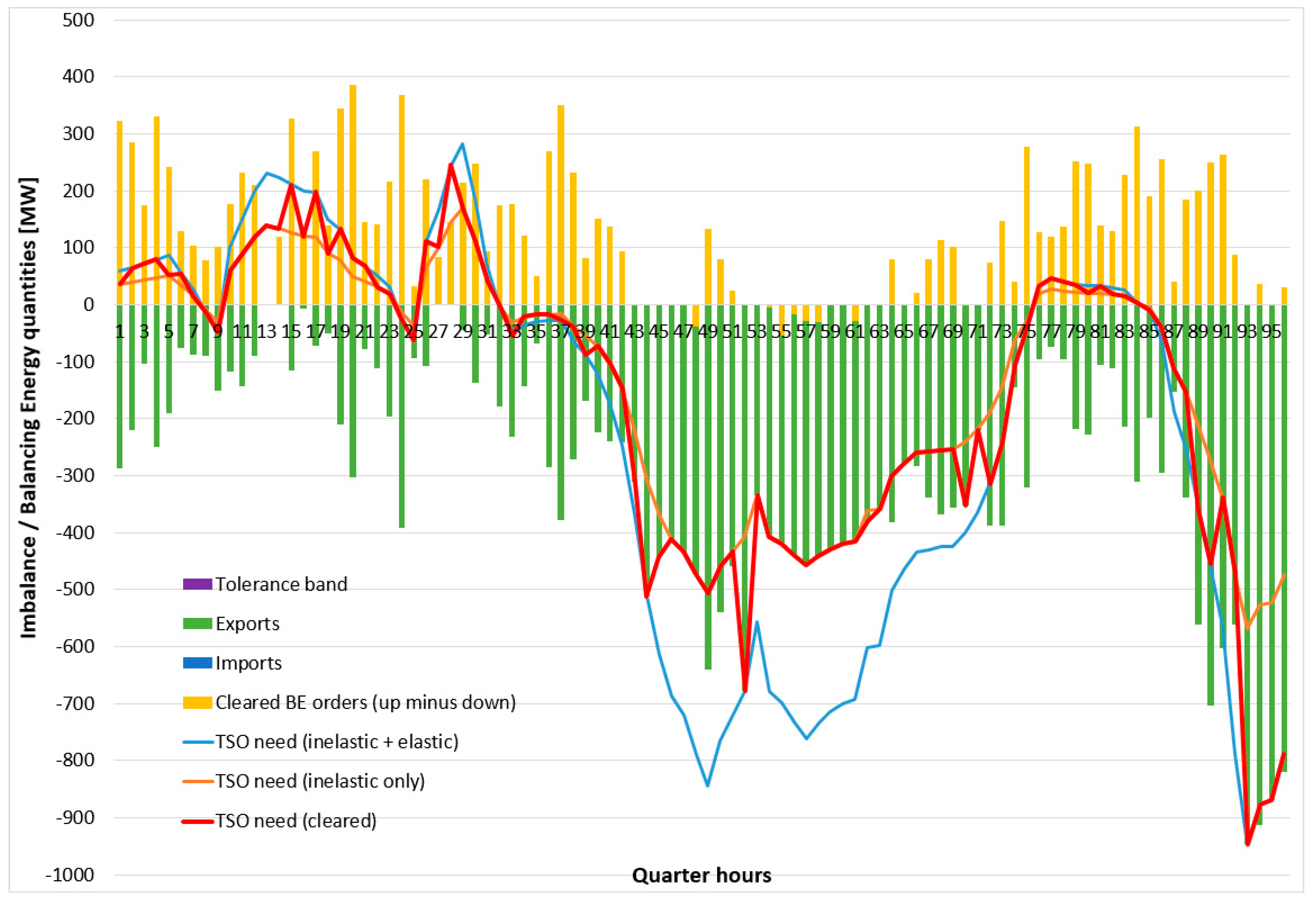
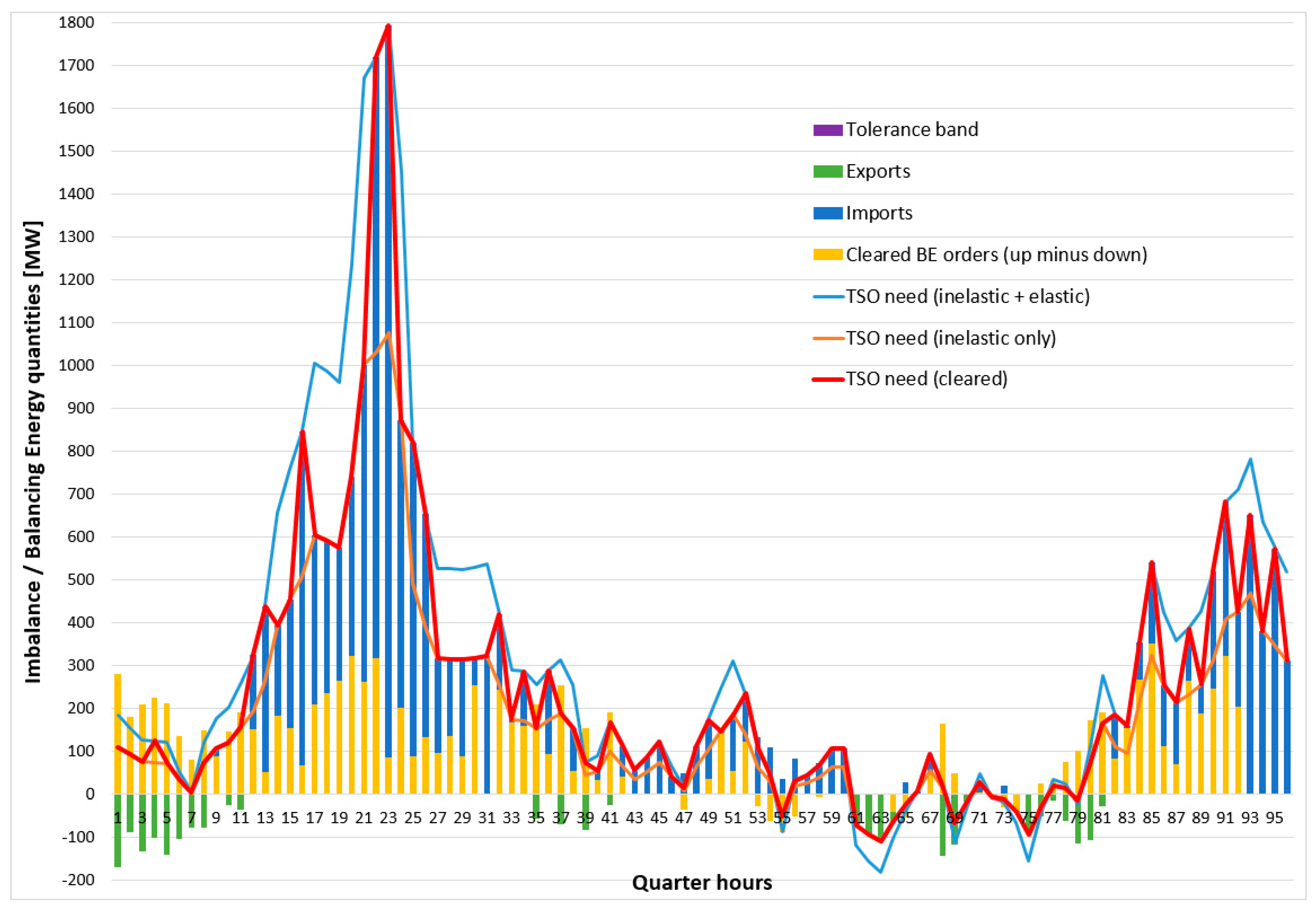
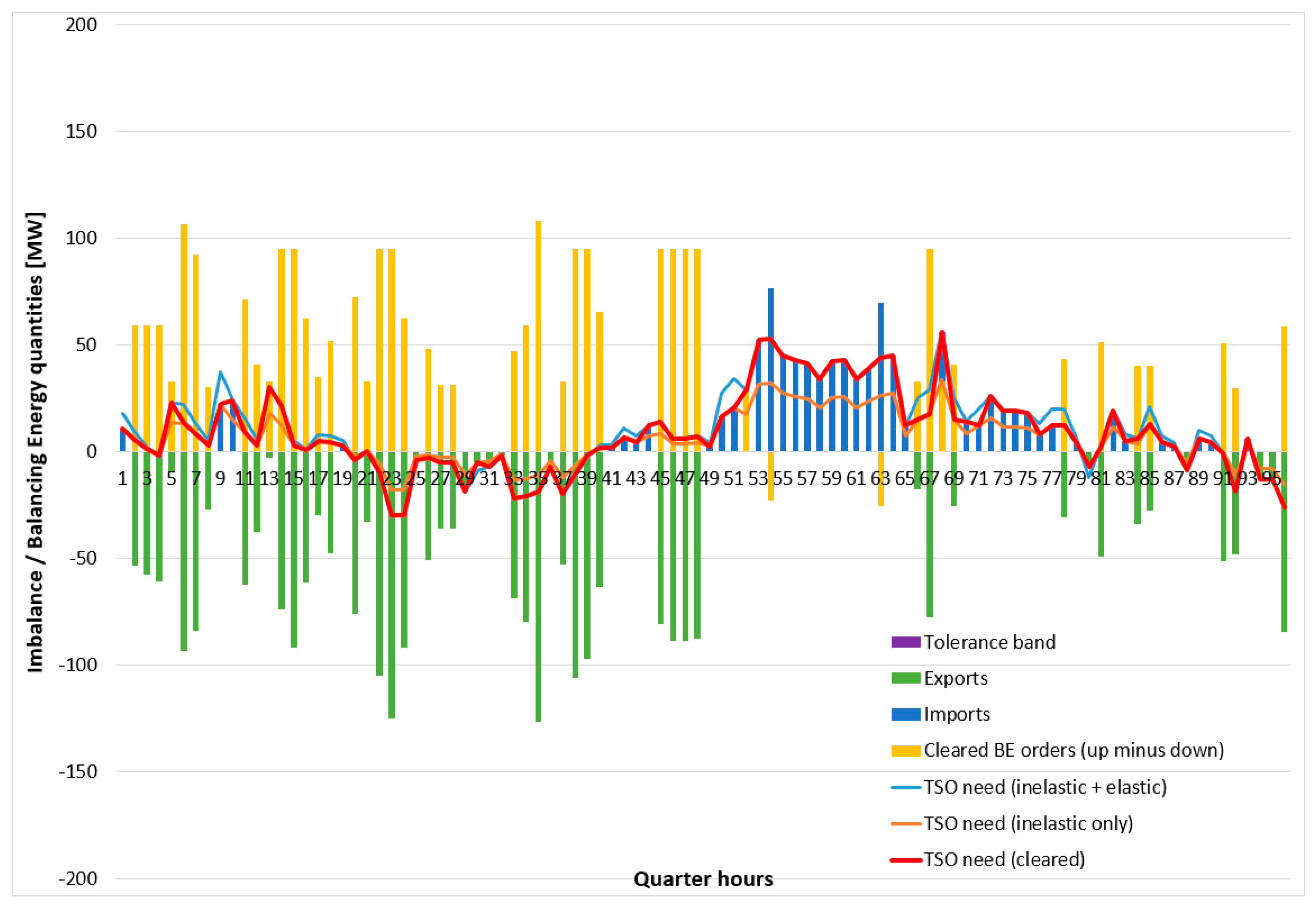
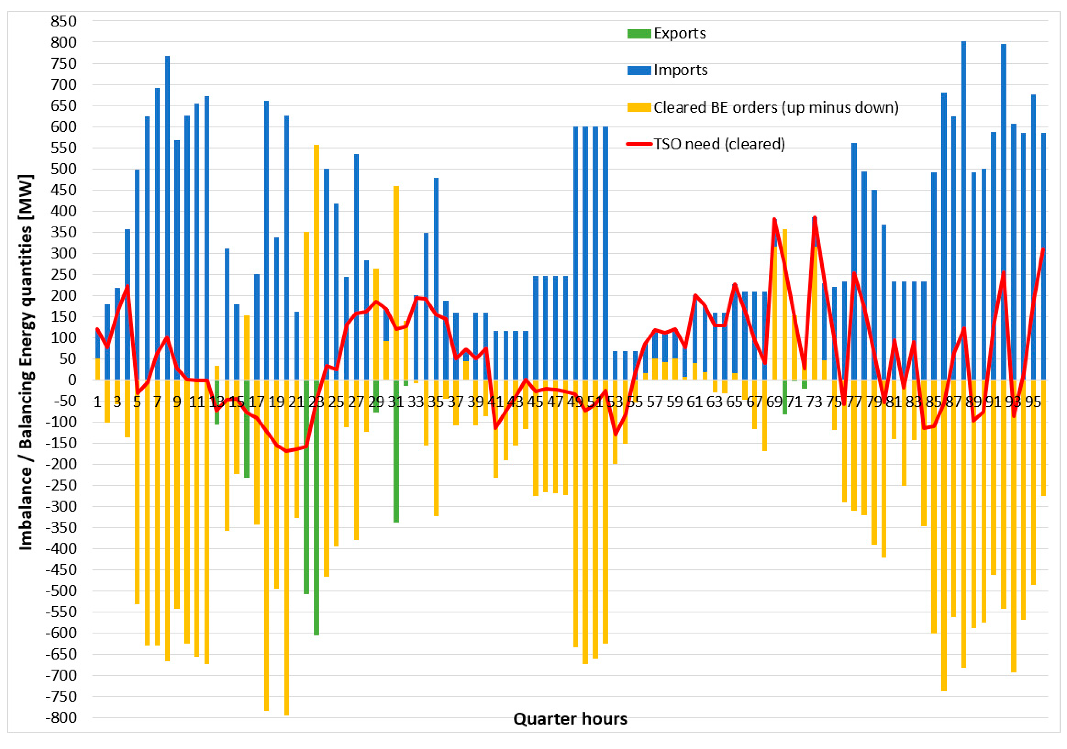
(b)

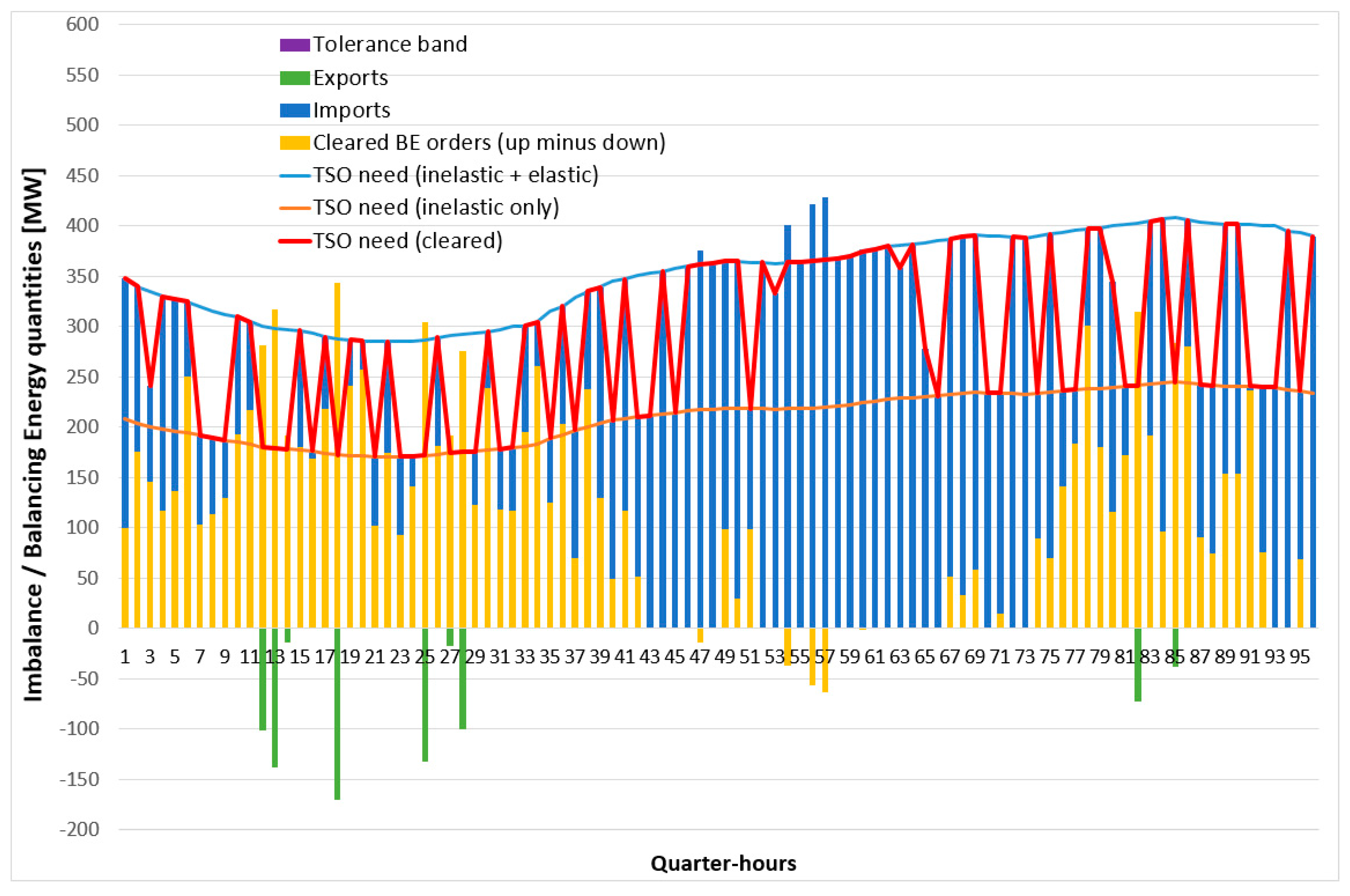
The activated BE from local or neighboring BSPs/BSEs covers the inelastic TSO need plus a portion (0–100%) of the elastic TSO need. The red bold line in Figure 11, Figure 12, Figure 13, Figure 14, Figure 15 and Figure 16 expresses the total cleared TSO need which always lies between the orange (inelastic TSO need) and blue (inelastic plus elastic TSO need) lines. The clearing status between these two lines depends on the order price of the elastic TSO needs and the respective BEO prices of BSPs.

(c)

The TSOs’ needs are covered by both local resources (orange bars) or by resources in neighboring countries (imports shown with blue bars), considering the available CZC of the interconnections. For example, in Portugal at the after-midnight (2–10) and night (19–21) h, the TSO needs are mainly covered by local resources, whereas at hours 11–18, these are mainly covered by imported BE from Spain.

(d)

In some cases, the local TSO needs may be quite small (e.g., in Switzerland), but the local resources are called to provide large amounts of upward BE to cover the needs of neighboring TSOs through respective exports (green bars in Figure 14).

(e)

In general, there are several cases where BSPs/BSEs are awarded upward BE (i.e., they are called to increase their production) to accommodate exports (e.g., in Switzerland and Greece), or inversely they are awarded downward BE (they are called to decrease their production) to accommodate imports (e.g., Italy).

(f)

The simultaneous cross-zonal BE procurement in regional basis levels the TSO needs’ spikes that may occur in a single market, by providing “support” from neighboring countries through respective imports/exports (depending on the sign of the TSO needs). This is evident, e.g., in France, where a large positive TSO need spike occurs at hours 4–7, which is mostly covered by imports from Switzerland and Spain. Actually, the TSO need is mostly “shaved” in a relatively low quantity (about 300 MW), and the local resources cover only the “shaved” TSO need.

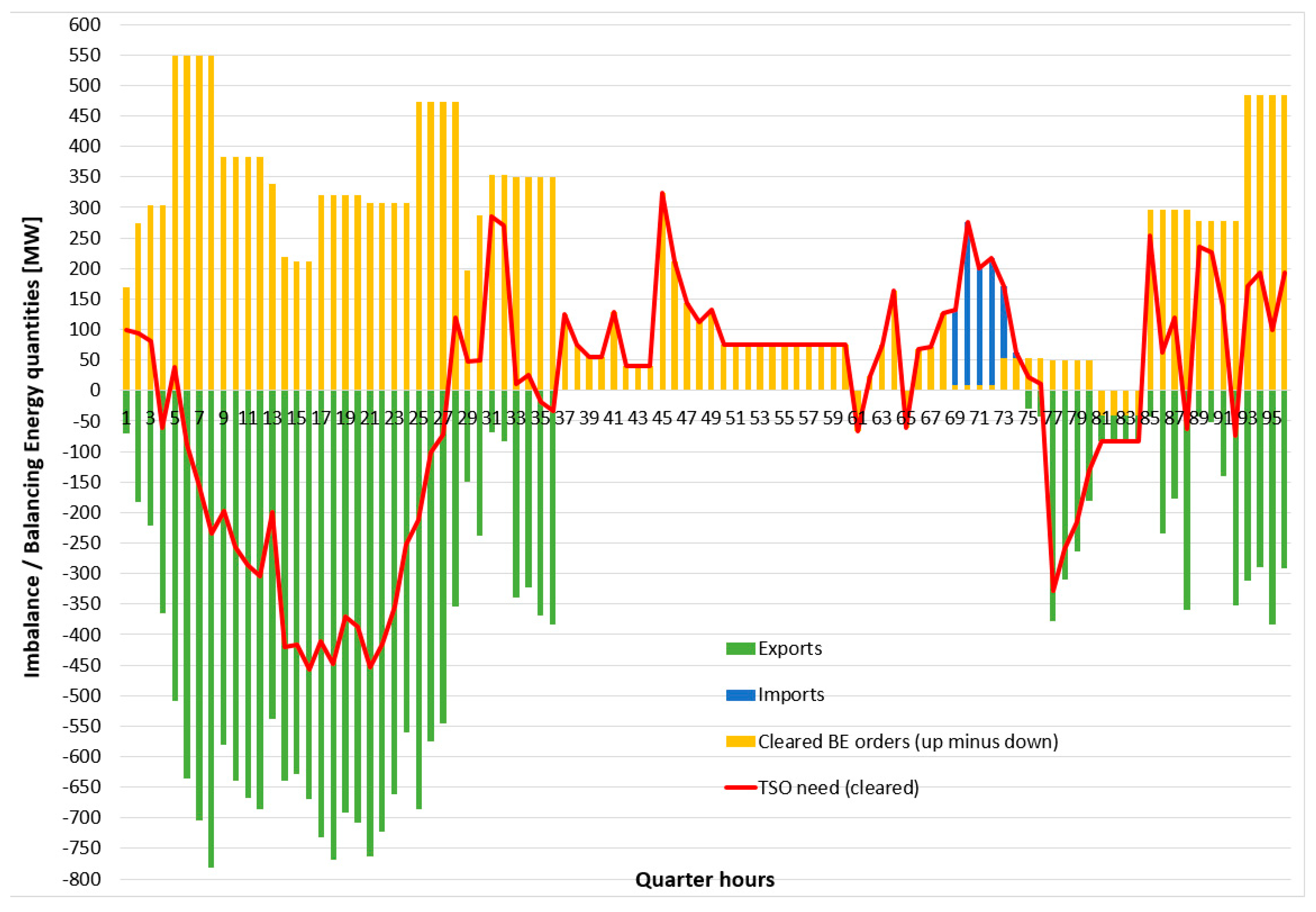
(g)

In the central-dispatch markets (Greece, Italy) there are no elastic TSO needs; hence, the Figure 15 and Figure 16 are simpler, containing only the cleared TSO need (which coincides with the inelastic TSO need), the local cleared BEOs and the imports/exports to neighboring markets. It should be noted that the mandatorily activated BEOs of such markets are included in the cleared BE quantities (orange bars) in both figures.

(h)

The orange lines internalize (net) any counter-activations due to the non-intuitive situation of upward BEOs being offered with a price lower than respective downward BEOs. The counter-activations provide a higher profit to TSOs, and the opportunity of such activations has been included in the LIBRA platform [17].

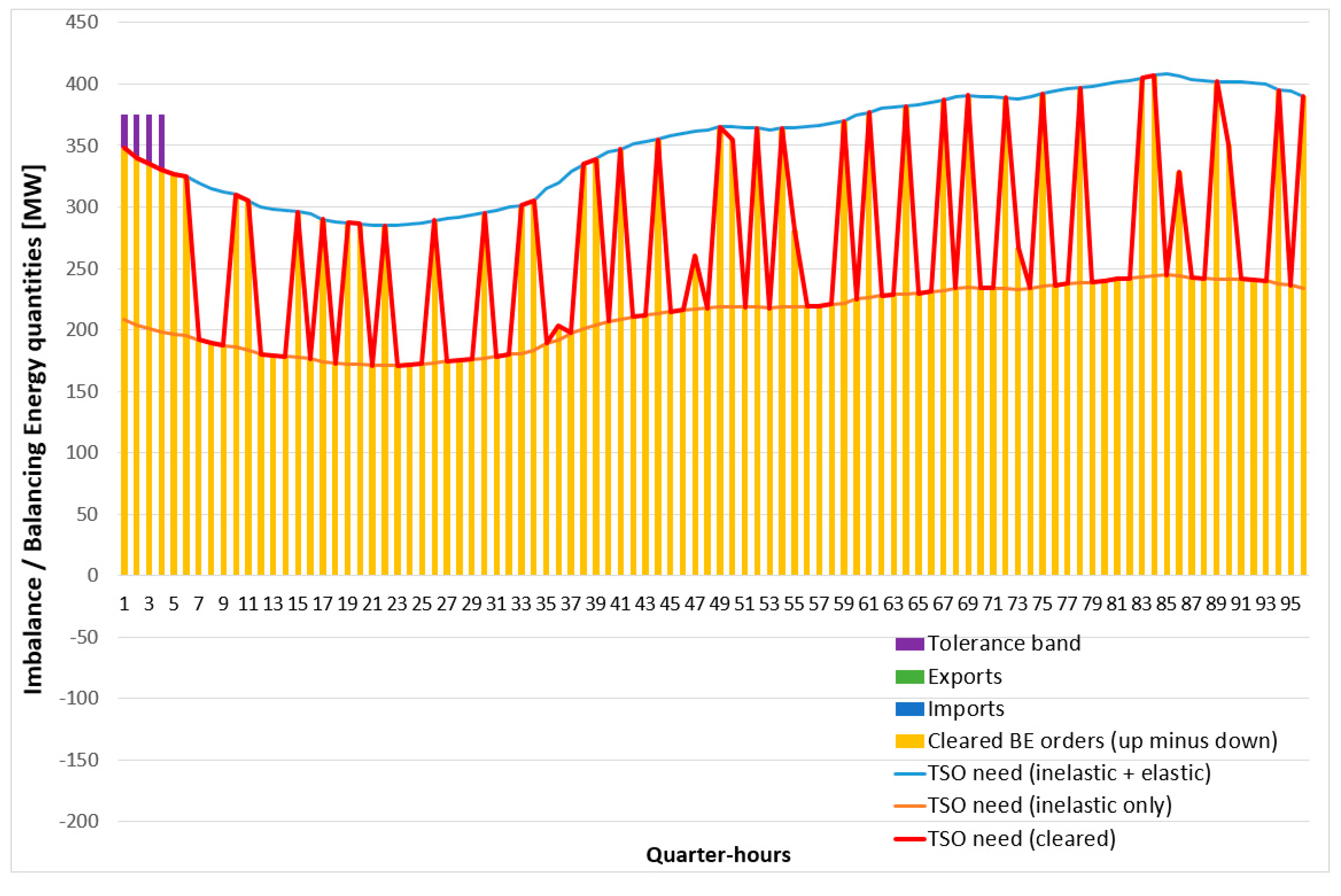
(i)

In a cross-zonal BE procurement scheme, it is highly unlikely that the tolerance band shall be used to ease the clearing process (in the presence of large indivisible blocks, as theoretically expected), due to the fact that imports/exports act implicitly as slack variables for a bidding zone’s imbalance needs, providing the necessary upward/downward flexibility to meet exactly the TSO’s needs without the activation of the tolerance band. The more interconnected a power system is (e.g., in central Europe with a meshed network), the easier it is to resolve the system’s imbalance needs using local or cross-border resources.

In order to highlight a case when the tolerance band is activated, the combination of the following data adjustments in the Portuguese market has been performed:

i.

the CZC with the neighboring country (Spain) has been zeroized in both directions for all RTUs;

ii.

the upward BEO quantity of an indivisible order has been set to a level (i.e., 375 MW) higher than the TSO needs for the 1st hour of the day, and the respective order price was reduced to a negative number (i.e., −2 €/MWh); and

iii.

all downward BEO prices have been decreased to levels below the order price referred in action (ii) above (i.e., lower than −2 €/MWh).

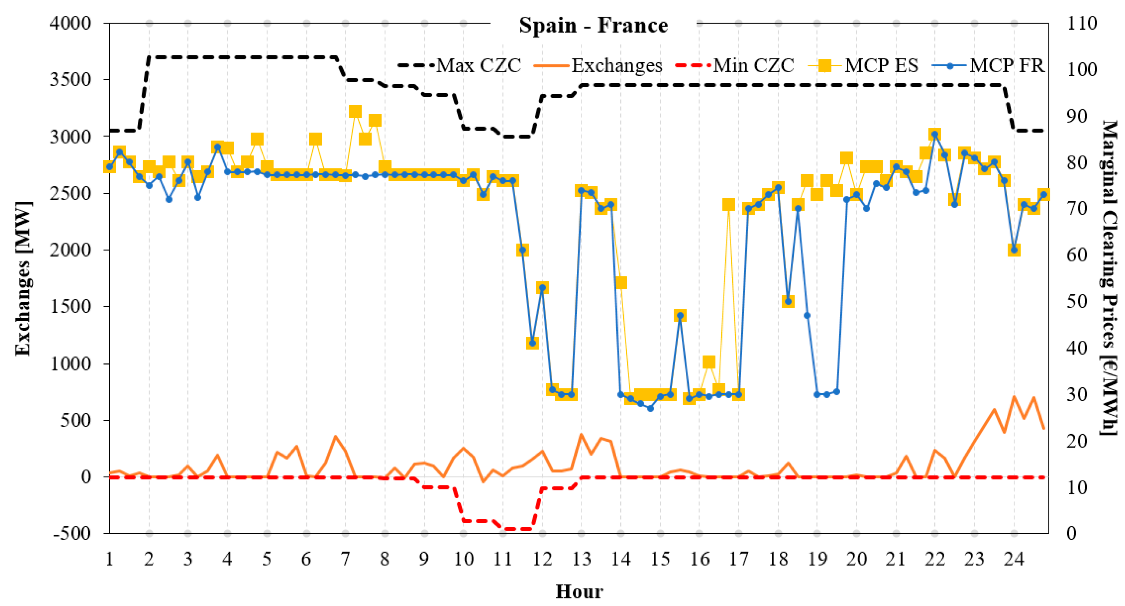
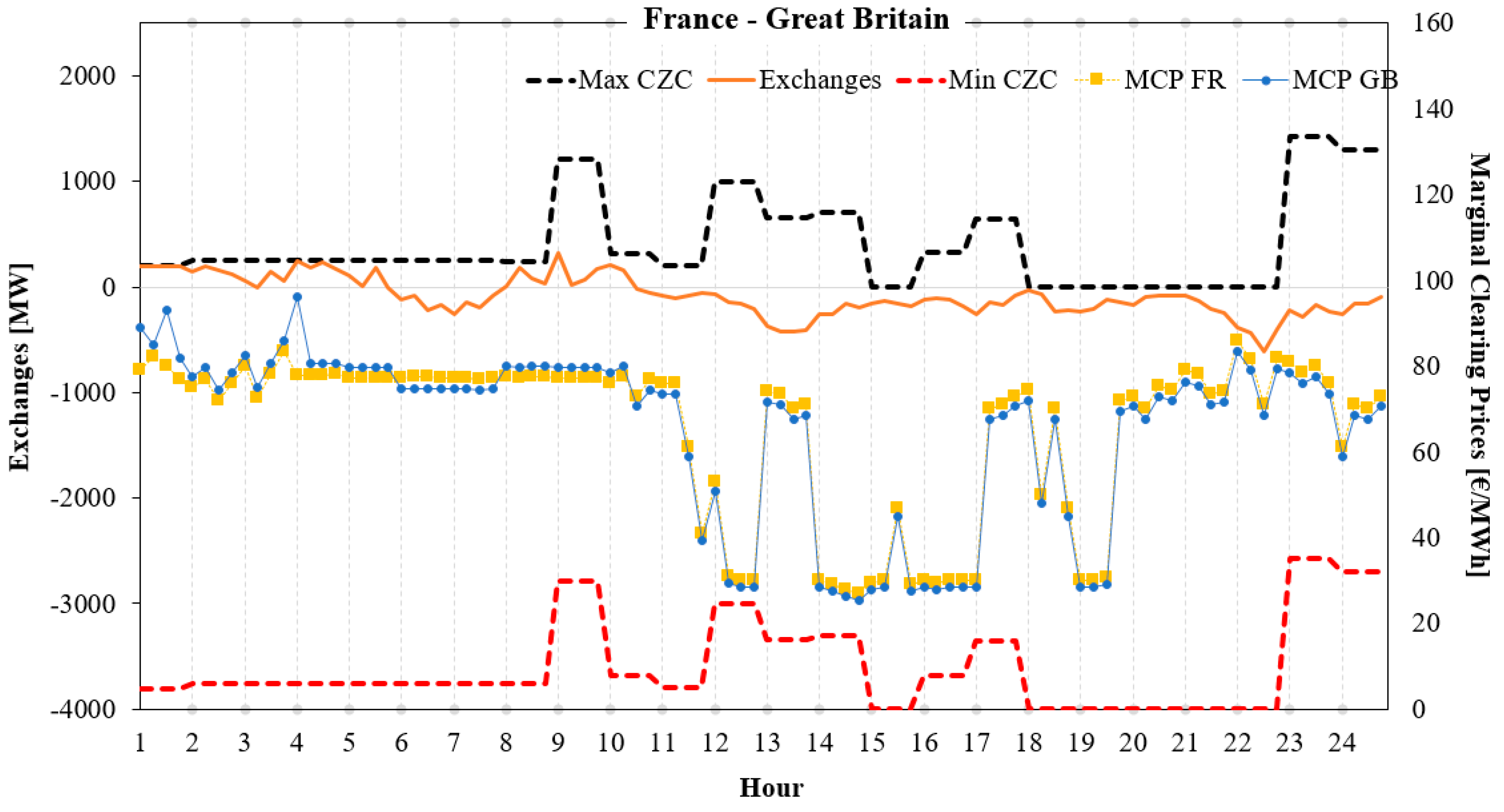
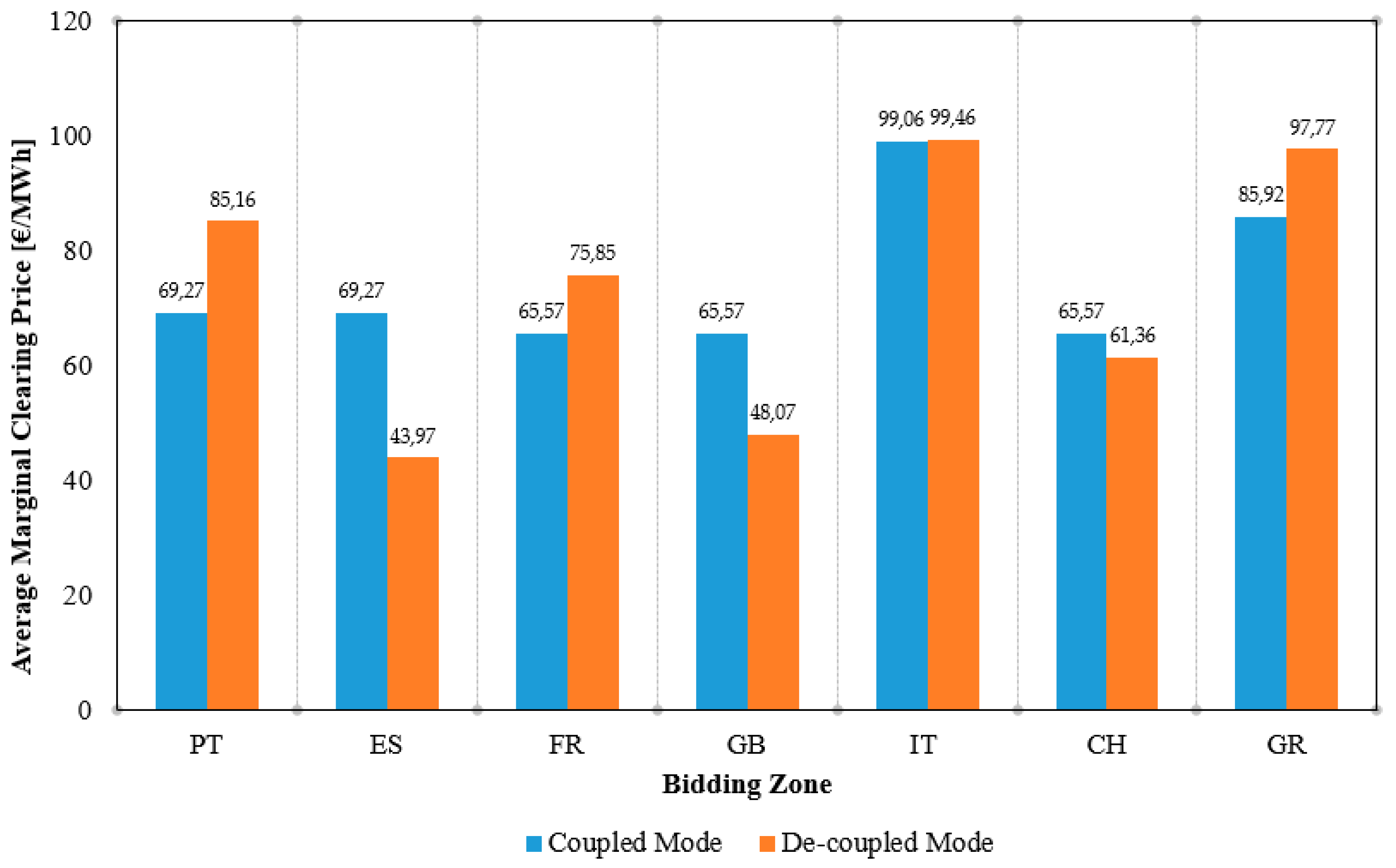
The combined effect of such actions led to the activation of the tolerance band in the first four RTUs of the day in Portugal (see Figure 17), where the acceptance of the large indivisible block of upward BE is more economically efficient than the activation of other smaller in quantity divisible/indivisible upward BEOs.

It should be noted that the available capacity of interconnections is usually covered in the prevailing direction by the long-term trades, as well as by the implicit day-ahead and intra-day sales/purchases in day-ahead and intra-day markets, respectively. However, this does not mean that there is no left CZC in the interconnections for cross-zonal BE exchanges. Actually, the non-prevailing direction is completely unutilized and thus can be used to cover neighboring regions’ imbalance needs in the appropriate direction. This is highlighted in Figure 18, where the CZC limits in both directions are illustrated in dashed black (maximum) and red (minimum) lines. In Figure 18, it is clearly shown that when there is enough CZC (e.g., at hours 10–12), the BE MCPs of the neighboring markets (which are defined as the shadow prices of the imbalance needs constraints) converge, whereas in cases of capacity shortage (e.g., at hours 19–20), the BE MCPs diverge.

Figure 19 illustrates another interesting case: in DC interconnections between France and Great Britain, even though the CZC is not constrained by the respective limits for many RTUs during the day, the BE MCPs do not fully converge, due to the DC interconnection line losses; specifically, when the exchange is positive (e.g., from France to Great Britain) the BE MCPs of France are lower than those of Great Britain. On the contrary, when the exchange is negative (e.g., from Great Britain to France), the BE MCPs are lower in Great Britain. In all cases, the cross-border procurement of RR BE:

(a)

leads to the full or partial convergence of MCPs. As illustrated in Figure 20, in the coupled mode, a price convergence (identical average MCPs) is observed between Portugal and Spain and between France, Great Britain, and Switzerland. On the other hand, in the de-coupled mode, such market areas attain different average MCPs for the reference day;

(b)

is beneficial from the TSO market perspective and thus for end-consumers, since it leads to higher overall social welfare. In our case, when a regional coupling is applied, the welfare amounts to 924,472.58 € while in an isolated mode (zero CZCs between bidding zones) the respective welfare equals to 523,671.87 €.

The above-mentioned findings verify the general argument that the harmonization of wholesale electricity markets across Europe would increase prices for some bidding zones and decrease prices for others. However, the ability to access the cheapest resources leads to increased social welfare.

5.2.2. Order Clearing Results

As far as the clearing status of submitted BEOs is concerned, in Figure 21 and Figure 22, we elaborate on two characteristic examples based on two different case studies. In the first, we consider a BSP in Portugal which submits three upward fully divisible orders for each RTU which are also exclusive in volume (i.e., they belong in the same group for each RTU). The first fully divisible order has a quantity of 200 MW per RTU (blue dotted line in Figure 21) and a price of 40 €/MWh; the second has a quantity of 350 MW per RTU (orange dotted line in Figure 21) and a price of 45 €/MWh; and the third has a quantity of 450 MW per RTU (yellow dotted line in Figure 21) and a price of 50 €/MWh. As shown in Figure 21, either the first or the second fully divisible order is exclusively accepted in each RTU among RTUs 41–76, to cover the TSO shortage. This is because these orders are more economic than the third fully divisible order. However, the latter order is exclusively accepted by the AOF during RTUs 77–92, when the needs for the Portuguese TSO are higher (higher black dotted line). It is worth noting that during such RTUs, the cleared quantity of the third fully divisible order is higher than the TSO need, meaning that energy is exported from Portugal to Spain. As shown, for all RTUs, only one of the three fully divisible orders is being accepted, thereby respecting the constraint imposed on exclusive in volume orders.

In the second test case, we consider again a BSP in Portugal which submits an upward linked in time divisible order for the first four RTUs (first hour of the scheduling period). This order has a quantity of 80 MW (blue columns in Figure 22) and a price of 40 €/MWh for each RTU. In addition, a minimum quantity is submitted per RTU as a minimum acceptance ratio (orange columns in Figure 22). As shown, during the first three RTUs, the Portuguese TSO has downward needs (system long), but the cleared quantity of the submitted upward order is non-zero. In fact, the acceptance ratio during such RTUs is affected by the acceptance ratio in the fourth RTU. Notably, during the fourth RTU, the TSO has upward needs, and thus, the order is accepted by the AOF to cover such needs. Consequently, due to the respective constraint imposed in linked in time orders, the acceptance ratio for all RTUs is the same and equal to 0.8. Such constrains help BSPs to schedule effectively their resources (i.e., respect the internal technical limitations of their BSEs), apparently to the detriment of the overall social welfare. Their scope is similar to resource operational limitations, such as ramping constraints, considered explicitly in the optimization algorithm of central-dispatch systems.

5.3. Computational Issues

The presented optimization model was solved on a desktop PC equipped with an i7/8-Core/4.0 GHz CPU processor and 16 GB of RAM, using the GAMS modeling software [47] and the CPLEX 12.9 solver (25.1.1, GAMS Development Corporation, Fairfax, VA, USA) with zero MIP optimality gap tolerance. Each hourly problem comprises 25,255 constraints with 6839 binary variables, 10,542 continuous variables, and 48,025 non-zero elements. The overall computational time for 24 consecutive hourly executions (practically 67 problem solutions considering the PAOs handling process and model re-executions for the elimination of PAOs) is equal to 70 s.

6. Conclusions

The modeling framework for the solution of the regional RR BE auctions (TERRE Activation Optimization Function) has been presented in this paper. Such framework is completely consistent with the provisions of the implementation framework [33] submitted by all TSOs participating in the TERRE project and approved by the respective NRAs. The novelty of this work compared to the existing literature lies mainly on the following contributions:

(a)

the inclusion of all order types of BEOs and the analytical mathematical representation of their clearing conditions;

(b)

the combination of self-dispatch and central dispatch market setups; for the latter, a pre-process is implemented before the clearing process for the conversion of BEOs to standard products (i.e., multi-part fully divisible orders) as required by EBGL;

(c)

the consideration of both elastic and inelastic orders submitted by the participating TSOs to cover their needs;

(d)

the inclusion of the tolerance band concept in the model constraints; and

(e)

the inclusion of ramping constraints for the central dispatch bidding zones in the overall regional clearing model for technical feasibility purposes.

The presented model has been tested on a case study including seven countries (Portugal, Spain, France, Great Britain, Switzerland, Italy, and Greece), in order to evaluate its performance on a large-scale real-world system. The results indicate that the model and the overall algorithm exhibit good escalation capabilities.

The attained results show that the cross-border RR BE procurement induces clearing prices convergence, which is attributed to the fact that more economical resources belonging to a bidding zone are instructed to cover needs from neighboring bidding zones. Additionally, the attained results indicate the significant effect of imbalance netting on the cleared BE quantities of BSPs in all markets with respect to the absolute TSO imbalance needs, which leads to a remarkable reduction in the costs incurred by the TSOs for real-time balancing purposes. This results in explicit savings for the Balance Responsible Parties (BRPs) paying the costs of balancing services provided to the TSOs and thus implicitly to the end-consumers through their energy tariffs.

The herein presented formulation can be deemed useful for the market stakeholders, in order for TSOs to operate it as a stand-alone application for analysis and benchmarking purposes and for Balancing Service Providers to simulate the AOF model and practice over multiple scenarios to maximize their gross profit from the provision of RR balancing energy.

References

1. European Commission. Market Legislation. Available online: https://bit.ly/2QDKDhg (accessed on 28 April 2020).
2. Booz and Company; Newbery, D.; Strbac, G.; Pudjianto, D.; Noel, P.; Fisher, L. Benefits of an Integrated European Energy Market. Available online: https://bit.ly/2QC3OYu (accessed on 28 April 2020).
3. Newbery, D.; Strbac, G.; Viehoff, I. The benefits of integrating European electricity markets. Energy Policy 2016, 94, 253–263. Available online: https://bit.ly/2sC95HJ (accessed on 28 April 2020). [CrossRef] [Green Version]
4. ENTSO-E. Implementation of Intraday and Day-Ahead Coupling as Well as Forward Capacity Allocation. Available online: https://bit.ly/2KMteQO (accessed on 28 April 2020).
5. ENTSO-E. Electricity Balancing. Available online: https://bit.ly/39AlHzQ (accessed on 28 April 2020).
6. ACER. Working towards a Single Energy Market to the Benefits of all EU Consumers. Available online: https://bit.ly/2QyrfC3 (accessed on 28 April 2020).
7. European Commission. Integration of Electricity Balancing Markets and Regional Procurement of Balancing Reserves. Final Report 2016. Available online: https://bit.ly/2rFQf1P (accessed on 28 April 2020).
8. Roben, F. Comparison of European Power Balancing Markets–Barriers to Integration. In Proceedings of the 15th International Conference on the European Energy Market, Łódź, Poland, 27–29 June 2018; Available online: https://bit.ly/2Q7U4Gz (accessed on 28 April 2020).
9. Esterl, T.; Kaser, S.; Zani, A. Harmonization issues for cross-border balancing markets: Regulatory and economic analysis. In Proceedings of the 13th International Conference on the European Energy Market, Porto, Spain, 6–9 June 2016; Available online: https://bit.ly/2Q7PRTg (accessed on 28 April 2020).
10. ENTSO-E. Commission Regulation (EU) 2017/2195 of 23 November 2017 Establishing a Guideline on Electricity balancing. Available online: https://bit.ly/3563hDD (accessed on 28 April 2020).
11. ENTSO-E. Frequency Containment Reserves. Available online: https://bit.ly/36c8j2L (accessed on 28 April 2020).
12. ENTSO-E. Imbalance Netting. Available online: https://bit.ly/2u5jmMZ (accessed on 28 April 2020).
13. ENTSO-E. PICASSO Project. Available online: https://bit.ly/2F7I7KA (accessed on 28 April 2020).
14. ENTSO-E. Manually Activated Reserves Initiative. Available online: https://bit.ly/3562UJf (accessed on 28 April 2020).
15. N-Side. MARI Algorithm Design Principles. Available online: https://bit.ly/3eqA2R2 (accessed on 28 April 2020).
16. ENTSO-E. TERRE Project. Available online: https://bit.ly/2QvOKM9 (accessed on 28 April 2020).
17. ENTSO-E. Explanatory Document to the Proposal of all Transmission System Operators Performing the Reserve Replacement for the Implementation Framework for the Exchange of Balancing Energy from Replacement Reserves. Available online: https://bit.ly/357gImv (accessed on 28 April 2020).
18. ACER. Annual Report on the Results of Monitoring the Internal Electricity and Natural Gas Markets in 2017. Available online: https://bit.ly/2ti7vKU (accessed on 28 April 2020).
19. ENTSO-E. An Overview of the European Balancing Market and Electricity Balancing Guideline. Available online: https://bit.ly/2W9zmYA (accessed on 28 April 2020).
20. N-Side. PCR and EUPHEMIA Algorithm. Available online: https://bit.ly/39pETjF (accessed on 28 April 2020).
21. Chatzigiannis, D.I.; Dourbois, G.A.; Biskas, P.N.; Bakirtzis, A.G. European day-ahead electricity market clearing model. Electr. Power Syst. Res. 2016, 140, 225–239. Available online: https://bit.ly/39oN9Al (accessed on 28 April 2020). [CrossRef]
22. Lam, L.H.; Valentin, I.; Bovo, C. European day-ahead electricity market coupling: Discussion, modeling, and case study. Electr. Power Syst. Res. 2018, 150, 80–92. Available online: https://bit.ly/36bpocX (accessed on 28 April 2020). [CrossRef]
23. Zani, A.; Migliavacca, G. Pan-European Balancing Market: Benefits for the Italian Power System. In Proceedings of the AEIT Annual Conference, Trieste, Italy, 19 September 2014; Available online: https://bit.ly/2F4WOhz (accessed on 28 April 2020).
24. Frade, P.M.S.; Shafie-khah, M.; Santana, J.J.E.; Catalao, J.P.S. Cooperation in ancillary services: Portuguese strategic perspective on replacement reserves. Energy Strategy Rev. 2019, 23, 142–151. Available online: https://bit.ly/39AnCV4 (accessed on 28 April 2020). [CrossRef]
25. Gebrekiros, Y.; Doorman, G. Balancing Energy Market Integration in Northern Europe—Modeling and Case Study. In Proceedings of the IEEE Power and Energy Society General Meeting, National Harbor, MD, USA, 27–31 July 2014; Available online: https://bit.ly/2sqdmOu (accessed on 28 April 2020).
26. Haberg, M. Optimal Activation and Congestion Management in the European Balancing Energy Market. Ph.D. Thesis, Norwegian University of Science and Technology, Trondheim, Norway, November 2019. Available online: https://bit.ly/3aJ7aB8 (accessed on 28 April 2020).
27. de Haan, J.E.S. Cross-Border Balancing in Europe: Ensuring Frequency Quality within the Constraints of the Interconnected Transmission System. Available online: https://bit.ly/39pr4BJ (accessed on 28 April 2020).
28. Jeriha, J.; Lakic, E.; Gubina, A.F. Innovative solutions for integrating the energy balancing market (mFFR). In Proceedings of the 16th International Conference on the European Energy Market, Ljubljana, Slovenia, 18–20 September 2019; Available online: https://bit.ly/2Qr2Oq0 (accessed on 28 April 2020).
29. Kannavou, M.; Zampara, M.; Capros, P. Modelling the EU Internal Electricity Market: The PRIMES-IEM Model. Energies 2019, 12, 2887. Available online: https://bit.ly/2syiNL9 (accessed on 28 April 2020). [CrossRef] [Green Version]
30. ELEXON. Project TERRE Implementation into GB Market Arrangements. Available online: https://bit.ly/2QytwgI (accessed on 28 April 2020).
31. RTE. TERRE Project. Available online: https://bit.ly/2MH7d78 (accessed on 28 April 2020).
32. ENTSO-E. Trans European Replacement Reserves Exchange (TERRE) project to deliver a European platform for the exchange of balancing energy from replacement reserves based on LIBRA solution live in January 2020. Available online: https://bit.ly/3fb94Oz (accessed on 28 April 2020).
33. ENTSO-E. The proposal of all Transmission System Operators Performing the Reserve Replacement Process for the Implementation Framework for the Exchange of Balancing Energy from Replacement Reserves. Available online: https://bit.ly/3c5eAzf (accessed on 28 April 2020).
34. ENTSO-E. Survey on Ancillary Services Procurement, Balancing Market Design 2018. Available online: https://bit.ly/2yh9zWv (accessed on 28 April 2020).
35. Marneris, I.G.; Biskas, P.N. Integrated Scheduling Model for Central Dispatch Systems in Europe. In Proceedings of the IEEE PowerTech Conference, Eindhoven, The Netherlands, 29 June–2 July 2015; pp. 1–6. Available online: https://bit.ly/2sxKpA5 (accessed on 28 April 2020).
36. Marneris, I.G.; Roumkos, C.; Biskas, P. Towards Balancing Market Integration: Conversion Process for Balancing Energy Offers of Central-Dispatch Systems. IEEE Trans. Power Syst. 2019, 35, 293–303. Available online: https://bit.ly/2F3cPEP (accessed on 28 April 2020). [CrossRef]
37. Genesi, C.; Marannino, P.; Montagna, M.; Rossi, S.; Siviero, I.; Zanellini, F. Coordinated implicit allocation of the CBTCs for the integration of the national European electricity markets. In Proceedings of the 2008 IEEE Power and Energy Society General Meeting—Conversion and Delivery of Electrical Energy in the 21st Century, Pittsburgh, PA, USA, 20–24 July 2008; pp. 1–8. Available online: https://bit.ly/3ddI9jt (accessed on 29 May 2020).
38. Meeus, L. Implicit auctioning on the Kontek Cable: Third time lucky? Energy Econ. 2011, 33, 413–418. Available online: https://bit.ly/2X92vVA (accessed on 29 May 2020). [CrossRef] [Green Version]
39. EuroPEX. Using Implicit Auctions to Manage Cross-Border Congestion: Decentralized Market Coupling. In Proceedings of the Tenth Meeting of the European Electricity Regulatory Forum, Rome, Italy, 8–9 July 2003; Available online: https://bit.ly/2M4UrPr (accessed on 29 May 2020).
40. Hoffler, F.; Wittmann, T. Netting of Capacity in Interconnector Auctions. Energy J. 2006, 28, 113–144. Available online: https://bit.ly/36EaFbD (accessed on 29 May 2020). [CrossRef] [Green Version]
41. Amprion Transmission System Operator. Multi Regional Coupling (MRC). Available online: https://bit.ly/3dhX5NL (accessed on 29 May 2020).
42. Hungarian Power Exchange. 4M Market Coupling Overview. Available online: https://bit.ly/36MOQXe (accessed on 29 May 2020).
43. Kath, C. Modeling Intraday Markets under the New Advances of the Cross-Border Intraday Project (XBID): Evidence from the German Intraday Market. Energies 2019, 12, 4339. Available online: https://bit.ly/3cfPduz (accessed on 29 May 2020). [CrossRef] [Green Version]
44. ENTSO-E. Transparency Platform. Available online: https://bit.ly/3bRsupu (accessed on 28 April 2020).
45. ENTSO-E. Mid-Term Adequacy Forecast 2019. Available online: https://bit.ly/2KOBDDn (accessed on 28 April 2020).
46. ResearchGate. TERRE AOF Input Data. Available online: https://bit.ly/3h1VyxC (accessed on 28 April 2020).
47. General Algebraic Modeling System. Available online: http://www.gams.com (accessed on 28 April 2020).
Figure 1. Replacement Reserves (RR) balancing process.
Energies 13 02966 g001
Figure 2. Balancing arrangements in the European countries (source [34]).
Energies 13 02966 g002
Figure 3. Example of a Common Merit Order List.
Energies 13 02966 g003
Figure 4. (a) Fully divisible order; (b) divisible order; (c) indivisible order.
Energies 13 02966 g004
Figure 5. Linked in time fully divisible order.
Energies 13 02966 g005
Figure 6. (a) Fully divisible order 1; (b) fully divisible order 2; (c) fully divisible order 3.
Energies 13 02966 g006
Figure 7. (a) Linked in time fully divisible order 1; (b) linked in time fully divisible order 2.
Energies 13 02966 g007
Figure 8. Exclusive in time fully divisible order.
Energies 13 02966 g008
Figure 9. Multi-part fully divisible order.
Energies 13 02966 g009
Figure 10. European balancing energy markets included in the test case.
Energies 13 02966 g010
Figure 11. Clearing results per Real-Time Unit (RTU) for Portugal.
Energies 13 02966 g011
Figure 12. Clearing results per RTU for Spain.
Energies 13 02966 g012
Figure 13. Clearing results per RTU for France.
Energies 13 02966 g013
Figure 14. Clearing results per RTU for Switzerland.
Energies 13 02966 g014
Figure 15. Clearing results per RTU for Greece.
Energies 13 02966 g015
Figure 16. Clearing results per RTU for Italy.
Energies 13 02966 g016
Figure 17. Clearing results per RTU for Portugal with clearing of Transmission System Operator (TSO) needs in the tolerance band.
Energies 13 02966 g017
Figure 18. Exchanges in the interconnection Spain–France and respective BE clearing prices.
Energies 13 02966 g018
Figure 19. Exchanges in the interconnection France–Great Britain and respective BE clearing prices.
Energies 13 02966 g019
Figure 20. Comparison of average Marginal Clearing Prices (MCPs) for the coupled and de-coupled modes.
Energies 13 02966 g020
Figure 21. Example of clearing of an exclusive in volume fully divisible order.
Energies 13 02966 g021
Figure 22. Example of clearing of a linked in time divisible order.
Energies 13 02966 g022