Figure 1.
(a) Co-simulation framework, (b) co-simulation process.
Figure 1.
(a) Co-simulation framework, (b) co-simulation process.
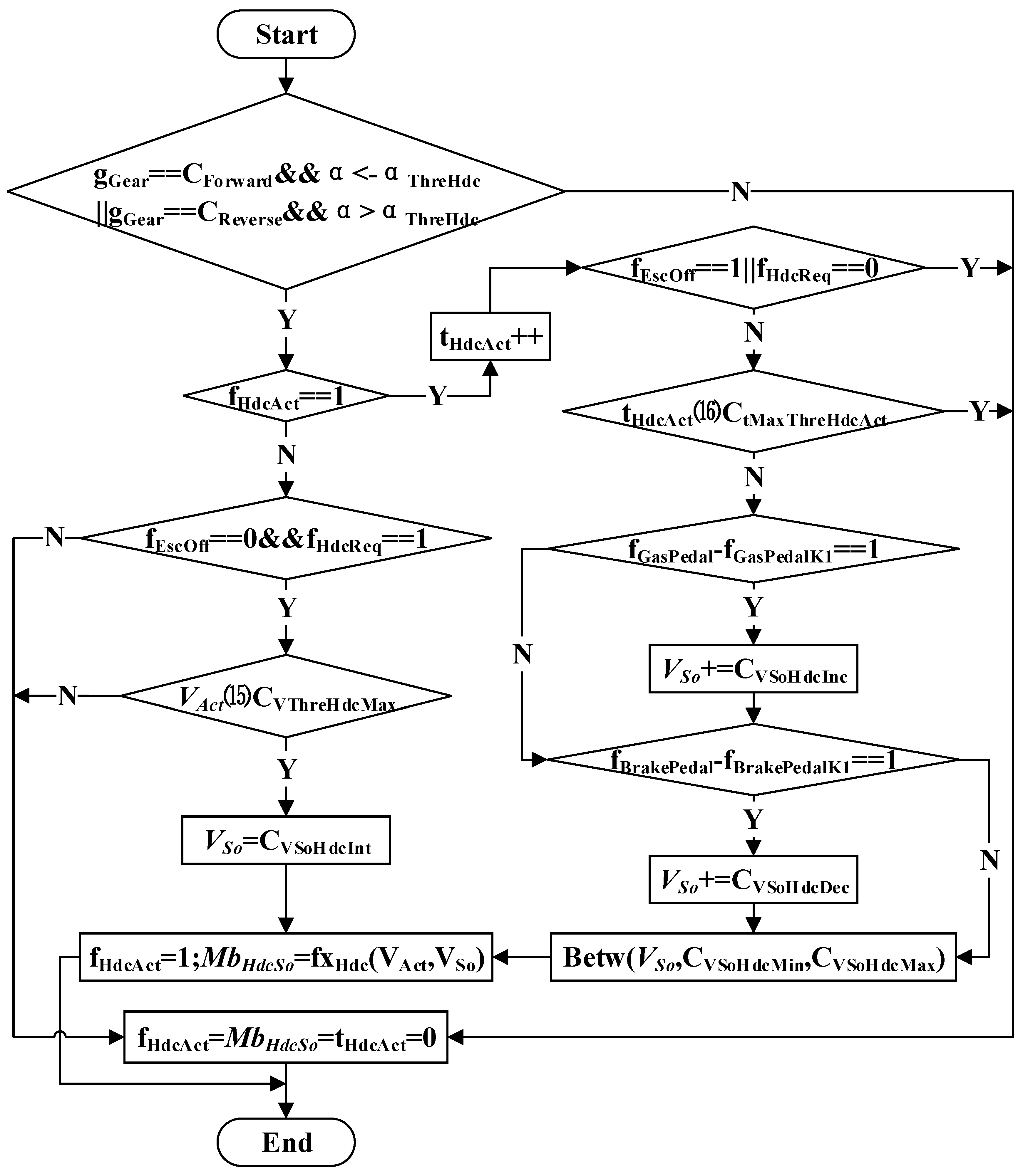
Figure 2.
Activation logic of HDC.
Figure 2.
Activation logic of HDC.
Figure 3.
Structure of proposed fuzzy-PID controller.
Figure 3.
Structure of proposed fuzzy-PID controller.
Figure 4.
Membership functions of E (a), EC (b), Kp (c), Ki (d) and Kd (e), respectively.
Figure 4.
Membership functions of E (a), EC (b), Kp (c), Ki (d) and Kd (e), respectively.
Figure 5.
Structure of proposed PID controller.
Figure 5.
Structure of proposed PID controller.
Figure 6.
Schematic diagram of hydraulic control unit (HCU).
Figure 6.
Schematic diagram of hydraulic control unit (HCU).
Figure 7.
The model of HCU built in AMESim.
Figure 7.
The model of HCU built in AMESim.
Figure 8.
Pressure corresponding to different duty of linear solenoid valve (USV).
Figure 8.
Pressure corresponding to different duty of linear solenoid valve (USV).
Figure 9.
The control logic of USV, switching solenoid valve (HSV) and motor.
Figure 9.
The control logic of USV, switching solenoid valve (HSV) and motor.
Figure 10.
The CarSim user interface.
Figure 10.
The CarSim user interface.
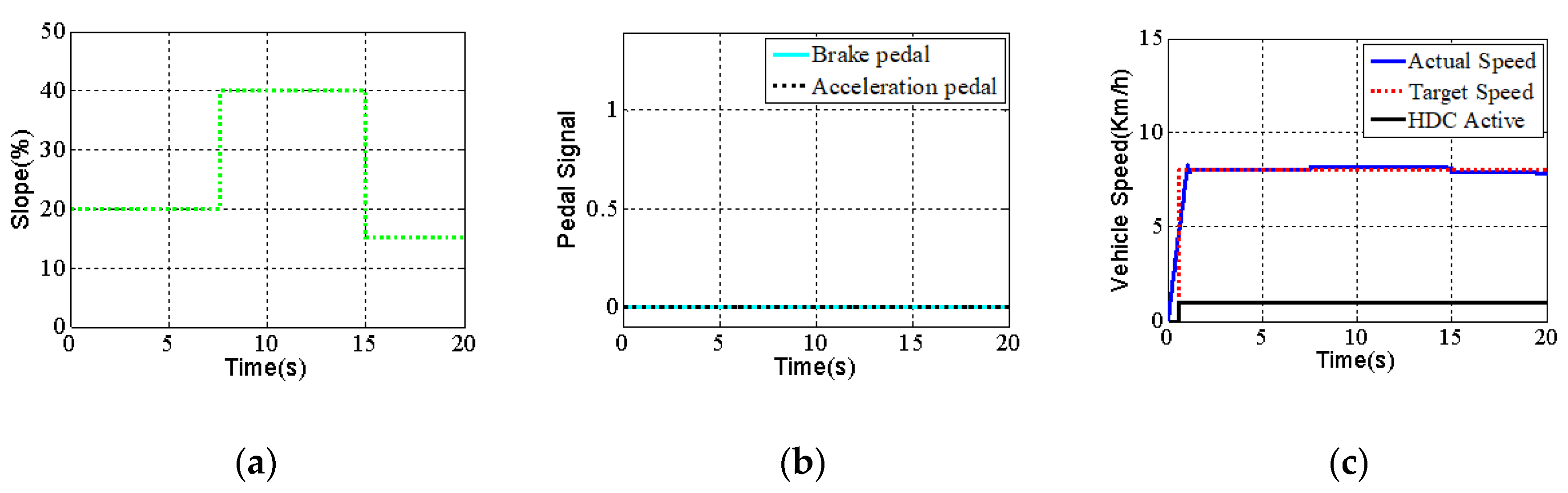
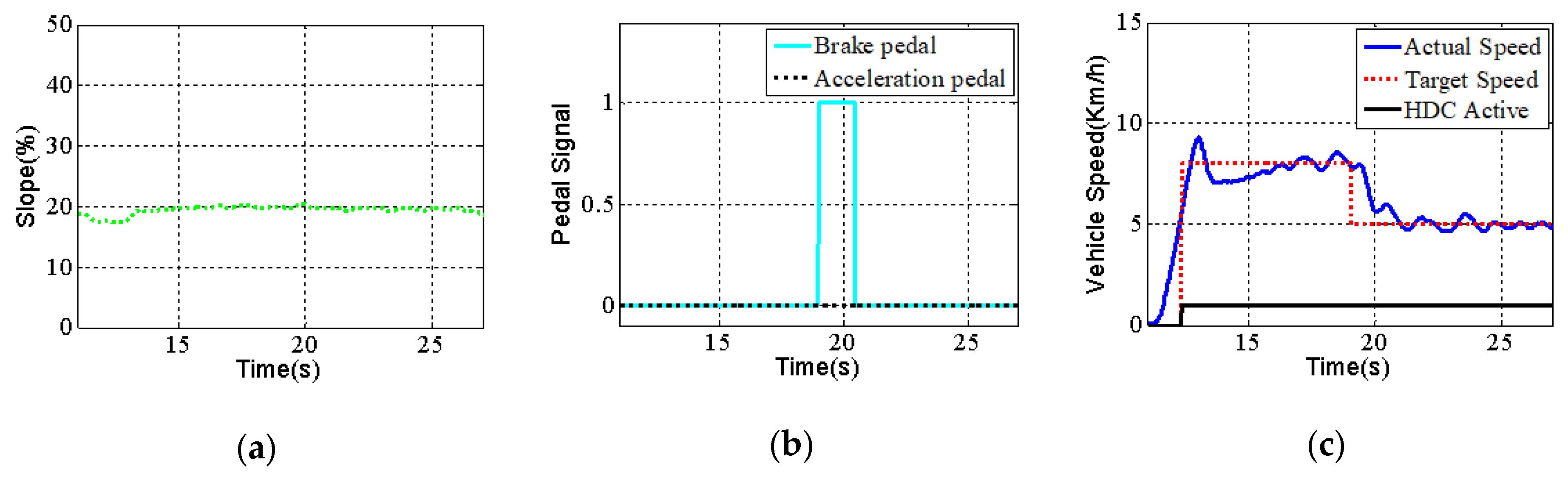
Figure 11.
Slope of ramp (a), brake and acceleration pedals signal (b), actual speed and target speed of the vehicle (c), the result carried out with fuzzy-PID controller.
Figure 11.
Slope of ramp (a), brake and acceleration pedals signal (b), actual speed and target speed of the vehicle (c), the result carried out with fuzzy-PID controller.
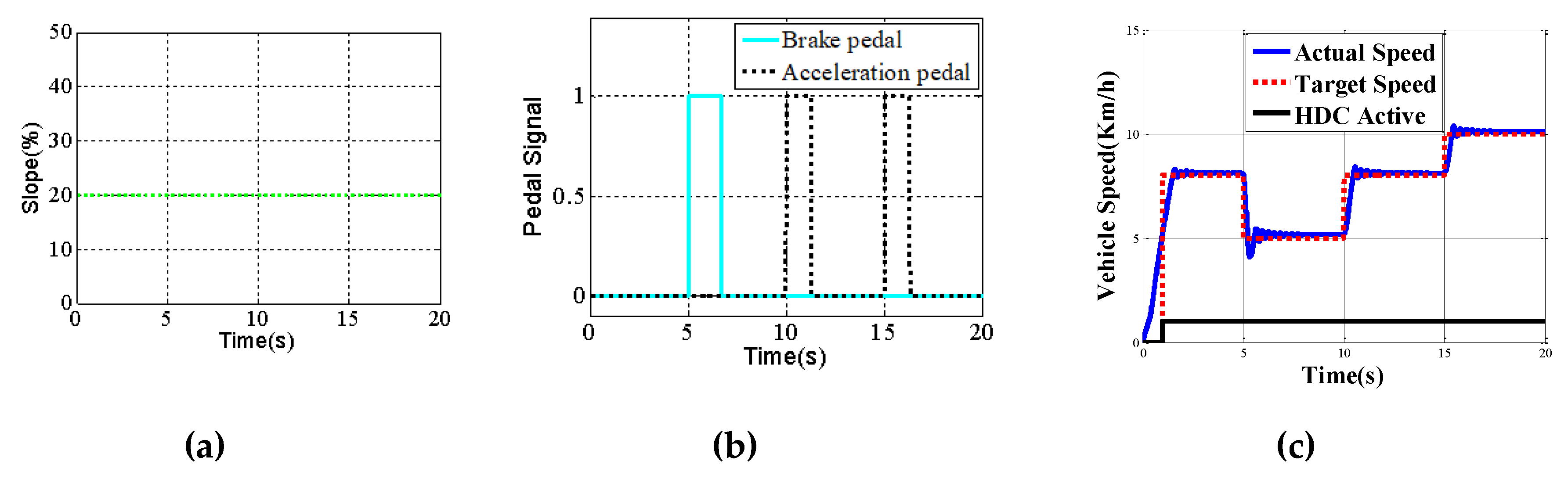
Figure 12.
Slope of ramp (a), brake and acceleration pedals signal (b), actual speed and target speed of the vehicle (c), the result carried out with fuzzy-PID controller.
Figure 12.
Slope of ramp (a), brake and acceleration pedals signal (b), actual speed and target speed of the vehicle (c), the result carried out with fuzzy-PID controller.
Figure 13.
Slope of ramp (a), brake and acceleration pedals signal (b), actual speed and target speed of the vehicle (c), the result carried out with PID controller.
Figure 13.
Slope of ramp (a), brake and acceleration pedals signal (b), actual speed and target speed of the vehicle (c), the result carried out with PID controller.
Figure 14.
Slope of ramp (a), brake and acceleration pedals signal (b), actual speed and target speed of the vehicle (c), the result carried out with PID controller.
Figure 14.
Slope of ramp (a), brake and acceleration pedals signal (b), actual speed and target speed of the vehicle (c), the result carried out with PID controller.
Figure 15.
Real figure of ESP (a), Structural explosion diagram of ESP (b).
Figure 15.
Real figure of ESP (a), Structural explosion diagram of ESP (b).
Figure 16.
Proving ground and the vehicle (a), the location where the ESP is installed on the vehicle (b).
Figure 16.
Proving ground and the vehicle (a), the location where the ESP is installed on the vehicle (b).
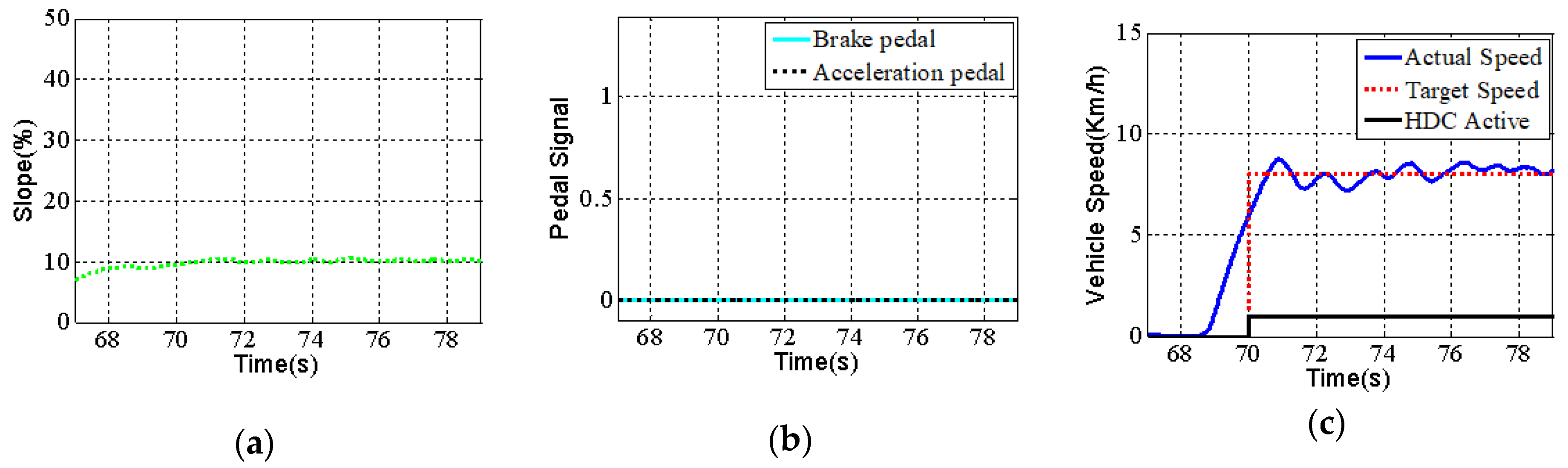
Figure 17.
Slope of ramp (a), brake and acceleration pedals signal (b), actual speed and target speed of the vehicle (c), at the slope of 10% and the driver does nothing with the pedal.
Figure 17.
Slope of ramp (a), brake and acceleration pedals signal (b), actual speed and target speed of the vehicle (c), at the slope of 10% and the driver does nothing with the pedal.
Figure 18.
Slope of ramp (a), brake and acceleration pedals signal (b), actual speed and target speed of the vehicle (c), at the slope of 15% and the driver does nothing with the pedal.
Figure 18.
Slope of ramp (a), brake and acceleration pedals signal (b), actual speed and target speed of the vehicle (c), at the slope of 15% and the driver does nothing with the pedal.
Figure 19.
Slope of ramp (a), brake and acceleration pedals signal (b), actual speed and target speed of the vehicle (c), at the slope of 20% and the driver does nothing with the pedal.
Figure 19.
Slope of ramp (a), brake and acceleration pedals signal (b), actual speed and target speed of the vehicle (c), at the slope of 20% and the driver does nothing with the pedal.
Figure 20.
Slope of ramp (a), brake and acceleration pedals signal (b), actual speed and target speed of the vehicle (c), the vehicle at the slope of 20% and the driver pushes the brake pedal at random.
Figure 20.
Slope of ramp (a), brake and acceleration pedals signal (b), actual speed and target speed of the vehicle (c), the vehicle at the slope of 20% and the driver pushes the brake pedal at random.
Figure 21.
Slope of ramp (a), brake and acceleration pedals signal (b), actual speed and target speed of the vehicle (c), the vehicle at the slope of 20% and the driver pushes the acceleration pedal at random.
Figure 21.
Slope of ramp (a), brake and acceleration pedals signal (b), actual speed and target speed of the vehicle (c), the vehicle at the slope of 20% and the driver pushes the acceleration pedal at random.
Table 1.
List of main symbols in this article.
Table 1.
List of main symbols in this article.
| Symbol | Description | Unit |
|---|
| Ax/g | The measured/Gravitational acceleration | m/s2 |
| gGear | The gear of vehicle | 1 |
| CForWard/CReverse | Forward/Reverse gears | 1 |
| α | The slope of ramp (The value is positive when the car’s nose is uphill and it is negative when downhill.) | 100% |
| θ | The angle of ramp | rad |
| αThreHdc | The threshold of slope of ramp | 100% |
| fHdcAct | The activation flag of HDC (The value is 1 when the HDC is motivated and 0 when HDC is shut down) | 1 |
| fEscOff | The close flag of ESC (The value is 1 when the ESC is open and 0 when ESC is shut down) | 1 |
| fHdcReq | The requirement flag of HDC (The value is 1 when the HDC is requested and 0 when it is not) | 1 |
| fxHdc | The function to calculate the target brake torque | 1 |
| hg | The height of vehicle center of mass | m |
| L | Wheel base | m |
| Lf/Lr | The distance between the front/rear axle and the center of mass | m |
| m | The mass of vehicle | Kg |
| VAct/VSo | Actual/Target vehicle speed | km/h |
| CVThreHdcMax | The maximum vehicle speed that HDC can be motivated | km/h |
| CVSoHdcInt | The initial target speed when HDC is motivated | km/h |
| MbHdcSo | Target brake torque | Nm |
| Pw | Actual brake pressure of wheel cylinder (From the pressure sensor) | bar |
| PSoAVe | Average target brake pressure | bar |
| PSof/PSor | The target pressure of the front rear axle | bar |
| PMaxf/PMaxr | The maximum pressure that the front/rear axle can withstand | bar |
| Pm | Master cylinder pressure | bar |
| Rf/Rr | The front/rear wheel radius | m |
| u | The road adhesion coefficient | 1 |
| CPThrInc | The threshold to increase the pressure of wheel cylinder | bar |
| CtMaxThreHdcAct | Maximum duration of HDC operation | s |
| fMotor | The motor start flag | 1 |
| fGasPedal/fBrakePedal | The flag of acceleration/brake pedal (The value is 1 when the pedal is pushed and 0 when the pedal is released) | 1 |
| fGasPedalK1/fBrakePedalK1 | The flag of acceleration/brake in the Last Cycle | 1 |
| CVSoHdcInc/CVSoHdcDec | Increment/Decrement value of target speed | km/h |
| CVSoHdcMin/CVSoHdcMax | Minimum/Maximum target vehicle speed | km/h |
| Kp/Ki/Kd | The proportional/integral/differential parameter | 1 |
| Cpf/Cpr | The front /rear axle ratio of brake torque to brake pressure | Nm/bar |
| DutyUSV/DutyHSV | The duty of USV/HSV | % |
| HDC | Hill descent control | 1 |
| PID | Proportion Integral Differential | 1 |
| ESP | Electronic stability program | 1 |
| E | The difference between the target speed and the actual speed | 1 |
| EC | The differential of the difference between the target speed and the actual speed | 1 |
| HCU | Hydraulic control unit | 1 |
| ECU | Electronic control unit | 1 |
| CAN | Controller area network | 1 |
Table 2.
Division of universe E.
Table 2.
Division of universe E.
| Membership Functions | NB | NM | ZO | PM | PB |
|---|
| Range | [–30 –20 –10 –2] | [–8 –3.5 0] | [–2 0 2] | [0 3.5 8] | [2 10 20 30] |
Table 3.
Division of universe EC.
Table 3.
Division of universe EC.
| Membership Functions | NB | NM | ZO | PM | PB |
|---|
| Range | [–20 –10 –5 –1] | [–3 –2 0] | [–1 0 1] | [0 2 3] | [1 5 10 20] |
Table 4.
Division of universe Kp.
Table 4.
Division of universe Kp.
| Membership Functions | O | S | M | B |
|---|
| Range | [–200 0 70] | [0 100 200] | [70 220 350] | [200 350 610 775] |
Table 5.
Division of universe Ki.
Table 5.
Division of universe Ki.
| Membership Functions | O | S | M | B |
|---|
| Range | [–8 0 5] | [0 5 12] | [5 10 16] | [12 16 24 30] |
Table 6.
Division of universe Kd.
Table 6.
Division of universe Kd.
| Membership Functions | O | S | M | B |
|---|
| Range | [–4 0 2] | [0 2 4] | [2 4 6] | [4 6 10 20] |
Table 7.
Kp rules of fuzzy control.
Table 7.
Kp rules of fuzzy control.
| EC Kp E | NB | NM | ZO | PM | PB |
|---|
| NB | S | S | M | S | O |
| NM | M | M | B | M | M |
| ZO | B | M | B | M | B |
| PM | M | M | B | M | M |
| PB | S | S | M | S | S |
Table 8.
Ki rules of fuzzy control.
Table 8.
Ki rules of fuzzy control.
| EC Kp E | NB | NM | ZO | PM | PB |
|---|
| NB | O | O | S | O | O |
| NM | O | S | M | S | O |
| ZO | S | M | B | M | S |
| PM | O | S | M | S | O |
| PB | O | O | S | O | O |
Table 9.
Kd rules of fuzzy control.
Table 9.
Kd rules of fuzzy control.
| EC Kp E | NB | NM | ZO | PM | PB |
|---|
| NB | O | M | B | M | O |
| NM | S | S | M | S | S |
| ZO | O | O | S | O | O |
| PM | S | S | M | S | S |
| PB | O | M | B | M | O |


