An Ensemble Stochastic Forecasting Framework for Variable Distributed Demand Loads

Abstract

Accurate forecasting of demand load is momentous for the efficient economic dispatch of generating units with enormous economic and reliability implications. However, with the high integration levels of grid-tie generations, the precariousness in demand load forecasts is unreliable. This paper proposes a data-driven stochastic ensemble model framework for short-term and long-term demand load forecasts. Our proposed framework reduces uncertainties in the load forecast by fusing homogenous models that capture the dynamics in load state characteristics and exploit model diversities for accurate prediction. The ensemble model caters for factors such as meteorological and exogenous variables that affect load prediction accuracy with adaptable, scalable algorithms that consider weather conditions, load features, and state characteristics of the load. We defined a heuristic trained combiner model and an error correction model to estimate the contributions and compensate for forecast errors of each prediction model, respectively. Acquired data from the Korean Electric Power Company (KEPCO), and building data from the Korea Research Institute, together with testbed datasets, were used to evaluate the developed framework. The results obtained prove the efficacy of the proposed model for demand load forecasting.

1. Introduction

Developments in the invasive use of grid-flexibility options, such as demand-side management (DSM), require pliability in load prediction mechanisms to match temporal and spatial differences between energy demand and supply [1]. Recent advancements in DSMs, such as vehicle-to-grid (V2G) technologies and renewable energy policies, induce new perspectives for energy demand-supply imbalance management [2]. A critical factor in this is the reliable prediction mechanism of demand loads [3]. Thus, much attention has been given to demand load forecast mechanisms over the past decade [4]. A significant drawback of these prediction mechanisms is the lack of reliable high-sampled historical demand data, unscalable predictive models to match consumption patterns, and insufficient information on load prediction state uncertainties [5,6]. Energy consumption differs among load types, consumption behavior, and time of energy usage. For loads with routine energy consumption, such as office building loads, the energy sequence is stationary with minimal energy variations within the operation periods. However, for non-routine energy consumption or generation loads, such as hotels and renewable power, respectively, the energy sequence is randomized, with many variabilities in the energy profile patterns. Such a situation can pose a challenge to predict with generalized prediction models.

Demand load forecasting is an established yet still very active research area [7]. The literature on prediction models on energy consumption is enormous, with recent studies harnessing the power of machine learning (ML) to develop highly-generalized predictive models. Before this, classical predictive methods dwelled mainly on statistical analysis [8,9,10]. Consumption patterns were stable with fewer variations with these loads; hence, models such as support vector regression (SVR) and auto-regressive integrated moving average (ARIMA) were used for short-term prediction of loads [11,12,13,14,15,16,17,18]. The relevance of these methods is dependent on the extensive dataset with collinear measuring variables, which, in most cases, are difficult to come by. Therefore, classical predictive methods were, as a result, incapable of capturing random variations in the data patterns [19]. Efforts to improve the forecasting methods incorporating such diversity and unevenness prompted attempts to replace classical regression models with ML techniques [20]. Predominate among these techniques is the artificial neural network (ANN). The ANN is already known for its dominant utilization in energy forecasting methods [13,21,22]. However, because of its inherent complexity, it mostly leads to overfitting. So, an ensemble model that harnesses the merit of ANN potential, together with other ML algorithms, could be devised for high accuracy load prediction. Recently, Wang et al. proposed an ensemble forecasting method for the aggregated load with subprofile [23]. In this work, the load profile is clustered into subprofiles, and forecasting is conducted on each group profile. Apart from the fact that this algorithm is based on a fine-grained subprofile, which may not be readily accessible from every energy meter, cluster members with similar features but different load profiles are problematic to cluster. Hence, a centroid representation of a cluster may lead to higher variance in load prediction. In [24], Wang et al. proposed a combined probabilistic model for load forecast based on a constrained quantile regression averaging method. This method is based on an interval forecast instead of a point forecast. Apart from increasing computational time required for bootstrapping, much data is needed, and interval resolution may not be optimal for other data. Given this, this paper focuses on a predictive ensemble with limited available historical datasets to develop a scalable online predictive model for demand load forecasting. In this study, date meta-data parameters and weather condition variables serve as inputs to the proposed framework. As opposed to the models mentioned above, the proposed prediction model is not based on any specific data sampling interval or strict prediction interval. The model is adaptable to different distributed demand loads with a varying number of predictors at various sampling intervals. The contributions of this study are to:

• Define an online stochastic predictive framework with a computation time of less than a minute.
• Define a prediction model capable of training a robust forecast model with a single or limited historical dataset.
• Define a prediction framework scalable and adaptable to different distributed demand load types.
• Define an error correction model capable of compensating forecast error.

The remainder of the paper is organized as follows. Section 2 discusses some challenges in demand load forecasting. Section 3 describes the probabilistic load forecasting model generation for stochastic demand load forecasting and error compensation methods. In Section 4, the results of the parametric models and the ensemble forecasting model on different case studies are presented.

2. Challenges in Load Forecasting

Load forecasting is a technique adopted by power utilities to predict the energy needed to meet generation to maintain grid stability. Data-gathering methods used in such an exercise are often unreliable, sometimes resulting in missing, nonsensical, out-of-range, and NaN(i.e., Not a Number) values. The presence of irrelevant and redundant information or noisy and unreliable data can affect knowledge discovery during the model training phase. The accuracy of forecasting is of great significance for both the operational and managerial loading of a utility. Despite many existing load forecasting methods, there are still significant challenges regarding demand load forecast accuracy. These challenges are data integrity verification, adaptive predictive model design, forecast error compensation, and dynamic model selection issues.

2.1. Unreliable Data Acquisition

Demand load forecasting is based on expected weather condition information. Accurate weather forecast is difficult to achieve because of changes in weather conditions from sudden natural occurrences. Thus, the demand load forecast may thus differ due to the actual weather condition information. Apart from the weather feature parameters, other forecasting features, such as data meta-data and consumed load, are required for demand load forecasting. The acquisition of this dataset could be unreliable due to the break-down or malfunctioning of energy meters. The dataset may thus contain non-sequential, missing, or nonsensical data. The consequential effects of such an event render the dataset highly unreliable and not suitable for accurate load forecasting.

2.2. Adaptive Predictive Modeling

Demand load forecasting complexities are influenced by the nature of the demand load, which is a result of consumer behavior changes, energy policies, and load type. The behavioral changes of energy consumers result in different energy usage patterns. For instance, building load type is determined by the hosted activities: commercial, residential, or industrial. Energy consumption in commercial and industrial buildings occurs in the light of routine activities that are derived from either uniform equipment operations or the implied consistency of organized human activities [25]. Demand load is affected by both exogenous (i.e., weather conditions) and endogenous (i.e., type of day) parameters [26,27]. With a stationary demand load, such as an office building load, energy consumption follows a specific pattern; hence, variability in energy consumption is not volatile.

Conversely, non-stationary buildings such as hotels have a high-frequency fluctuation in their energy demand sequence because of randomized operation conditions, such as varying occupancy levels. The changing pattern leads to poor prediction accuracy with an unscalable predictive algorithm. To mitigate such problems, conventionally, for grid load forecast, utility operators use manual methods that rely on a thorough understanding of a wide range of contributing factors based on upcoming events or a particular dataset. Relying on manual forecasting is unsustainable due to the increasing number of complexities of the prediction. Hence, the predictive model for load should be adaptive to the changing conditions.

2.3. Transient-State Forecast Error

The estimated load forecast may change as a result of a sudden natural occurrences, such as tsunami, typhoons, or holidays. Such changes are temporary and may not occur often. Thus, the day-ahead predictive parameters may not reflect these sudden changes. Hence, the predictive model forecast may deviate from the expected forecast. The predictive model captures only steady-state parameters when the load is modeled to fit historical data. The steady-state predictive model ignores transient forecast errors. Such a phenomenon significantly reduces the accuracy of the load forecast.

2.4. Model Selection Criteria

All statistical forecasting methods could be used to fit a model on a dataset. However, it is difficult to fit a model that captures all the variabilities in a demand load dataset, considering the numerous complex factors that influence demand load forecasting. Additionally, obtaining accurate demand load forecasts based only on parameters such as weather information and other factors that influence consumption may not always be correct since, under certain circumstances, some predictive models have higher prediction accuracy than others. Hence, the criteria for selecting the best fit model under certain conditions is critical for accurate demand load forecasting. Given this, various methods are proposed in this framework to address these challenges, as mentioned earlier.

3. Probabilistic Load Forecasting Model Generation

In this study, we based our proposed framework on the ensemble forecasting method. The proposed forecasting framework, as shown in Figure 1, involves the process of demand consumption data and weather information acquisition, data integrity risk reduction, forecast error compensation, point-forecast, and stochastic forecast estimation. The ensemble forecasting method is an integration of a series of homogenous parametric models as a random forecast model [24]. The set of parallel parametric models train and forecast load independently. In this study, the forecasting process is in two stages: point-forecast model generation and ensemble processes. The point-forecast generation process involves mechanisms in generating deterministic forecasts with point-forecast models. This process comprises parametric model selection techniques and data integrity risk reduction methods. With the ensemble process, the model scheme defines strategies for optimal forecast model selection, forecast error compensation, and stochastic forecasts. Since parametric model selection is not the primary consideration of this study, we introduce only three typical parametric models. In the last decade, several parametric models have been selected for demand load predictive modeling. Notable among them are the artificial neural network (ANN), K-means, and Bayesian [28,29,30,31,32,33,34,35,36,37,38,39] approaches. The choice of these models for demand load prediction is because of their acute sensitivity to sequential data prediction. Our proposed framework is adaptable to multiple parametric or meta-parametric models for the efficient prediction of sequential demand load.

3.1. Data Integrity Risk Reduction

As part of the study, preprocessing analysis was performed on the dataset to increase the integrity of the dataset. We defined a risk reduction method as part of this study to detect outliers and also compensate for irregular or missing data. The first stage of the risk reduction method deals with data outlier detection. The acquired demand load data contains outliers because of measurement latencies, changes in systems behavior, or fault in measuring devices. In this study, boxplot and generalized extreme studentized deviate (ESD) algorithms were adopted to detect irregularities in the demand load data. These methods are common statistical techniques used to identify hidden patterns and multiple outliers in data [40]. The technique depends on two parameters, $\alpha$ and $r$, being the probability of false outliers and the upper limit of expected number of potential outliers, respectively. As mentioned by Carey et al. [41], the maximum number of potential outliers in a dataset is defined by the inequality in Equation (1).

$$r<0.5\left(n-1\right)$$

(1)

where n is the number of observations in the data set. With the upper bound of $r$ defined, the generalized ESD test performs r separate tests: a test for one outlier, two outliers, and so forth up to $r$ outliers.

$$X:\left\{x_1,x_2,x_3,\dots ,x_n\right\}$$

(2)

For each r separate test, we compute the test statistic, $R_i$, that maximizes $\left|x_i-\overline{x}\right|$ for all observations as specified in Equation (3), where $\overline{x}$ and $s$ denote the sample mean and the standard deviation, respectively. The observation $x_i$ that maximises $R_i$ is then removed and $R_i$ recomputed with $\left(n-1\right)$ observations. This process is repeated for all $r$ with the outcome test statistics of $R_1,R_2,\cdots ,R_r$.

$$R_i=\frac{max\left|x_i-\overline{x}\right|}{s}$$

(3)

The critical value, ${\lambda }_i$, is therefore computed for each $r$ test statistic in Equation (4) with tail area probability, $p$, defined in Equation (5), where $t_{p,n-i-1}$ is the 100$p$ percentage point from the t-distribution with (n − i − 1) degrees of freedom. The pair of test statistics and critical values are arranged in descending order. The number of outliers is therefore determined by finding the largest $i$ such that $R_i>{\lambda }_i$.

$${\lambda }_i=\frac{\left(n-1\right)t_{p,n-i-1}}{\sqrt{\left(n-i-1+t_{p,n-i-1}^2\right)\left(n-i+1\right)}}; \forall i\in r$$

(4)

$$p=1-\left[\frac{\alpha }{2\left(n-i+1\right)}\right]$$

(5)

Following the outlier detection is the data imputation method. Missing data as a result of outlier removal or sampling error are compensated for with the data imputation method. Using demand load profiles with missing data can introduce a substantial amount of bias, rendering the analysis of the data more arduous and inefficient. The imputation model defined in this study preserves the integrity of the load profiles by replacing missing data with an estimated value based on other available information. The proposed reduction model in this study is in three stages of imputation: listwise deletion, hot-deck, and Lagrange regression model.

For training analysis, from a dataset $X$ with feature variables M and number of observations N, the listwise deletion method deletes a set of records with missing data values of any of the feature variables. The listwise deletion method produces a reduced dataset, $X^{*}$, as defined in Equation (6).

$$X^{*}=\left[X_1^{*}, X_2^{*},\cdots X_j^{*}\right]; \forall j\in N$$

(6)

$$X_j^{*}=X_j :\exists l_{i,j}\cap \exists l_{i+1,j}\cap \cdots \cap \exists l_{i+m,j}=1$$

(7)

$$l_{i,j}=\{\begin{array}{cc}1;\hfill & \exists x_{i,j}\forall i\in M\hfill \\ 0;\hfill & \nexists x_{i,j}\forall j\in N\end{array}$$

(8)

This process does not cause bias, but decreases the power of the analysis by reducing the sufficient sample size. For continuous missing data values (i.e., >3, based on the sampling interval), the listwise method could introduce bias. Thus, for a single missing value, the hot-deck technique is adapted—the hot-deck procedure imputes missing values with previously available data of the same feature variable as defined in Equation (9). The hot-deck technique precedes the listwise deletion method.

$$X^{*}=\left[X_1^{*}, X_2^{*},\cdots X_j^{*}\right]; \forall j\in N$$

(9)

$$X_j^{*}=\left[X_{1,j}^{*},X_{2,j}^{*},\cdots X_{m,j}^{*}\right]; \forall m\in M$$

(10)

$$x_{i,j}^{*}=\{\begin{array}{cc}{x}_{i,j};\hfill & \exists x_{i,j}\forall i\in M\hfill \\ x_{i,j-1};\hfill & \nexists x_{i,j}\forall j\in N\hfill \end{array}$$

(11)

For multiple data imputation, an ensemble method made up of regression and Lagrange imputation was adapted. There are seasonal, cyclic, and trend patterns in a demand load dataset. With a week-ahead daily load profile, as depicted in Figure 2, the similarity in the patterns of the two load profiles of the same season and day type is evident. Thus, from the immediate prior week, daily load profile information could be used to estimate missing data values in the week-ahead daily load profile.

To achieve this, we estimated the missing data values with a regression imputation method based on the observed values. However, the perfect prediction regression equation is impractical in some situations (e.g., with a limited number of observations). Hence, the standard error associated with the forecast can be reduced with the demand profile of the previous week. Thus, we estimated the deviation and the rate of deviation, R, of the previous demand load profile. From this, we defined a Lagrange imputation model with the load deviation rate as defined in Equation (12). The initial predicted missing values are modified with the Lagrange model, as shown in Figure 3.

$$\begin{array}{c}y=\frac{\left(R-R_2\right)\left(R-R_3\right)\cdots \left(R-R_n\right)}{\left(R_1-R_2\right)\left(R_1-R_3\right)\cdots \left(R_1-R_n\right)}{y}_1+\\ \frac{\left(R-R_1\right)\left(R-R_3\right)\cdots \left(R-R_n\right)}{\left(R_2-R_1\right)\left(R_2-R_3\right)\cdots \left(R_2-R_n\right)}{y}_2+\cdots +\frac{\left(R-R_1\right)\left(R-R_2\right)\cdots \left(R-R_{n-1}\right)}{\left(R_n-R_1\right)\left(R_n-R_2\right)\cdots \left(R_n-R_{n-1}\right)}{y}_n\end{array}$$

(12)

The estimated error margin for each continuous range of imputation is (MAPE: 0.22, MAE: 7.14) and (MAPE: 0.08, MAE: 8.24) for the first and second ranges, respectively. With the estimated margin errors, it is evident that the reduction method could be used to compensate for data irregularities.

3.2. Feature Variable Selection

Many predicting features affect energy consumption. For instance, date meta-data features, such as the time of day, type of day, season, and weather conditions, correlate with energy consumption. The selection of such input parameters is critical to the performance of the predictive model. Uncorrelated or associated parameters may not only lead to model overfitting but affect the performance of the predicting model [42,43]. The set of variables for this study, described in

Table 1. Features description.

Variable Type	Variable Name	Value
Predictors	Year	4-digit number year. E.g., 2017
	Month	2-digit number month. E.g., 01
	Day	2-digit number day. E.g., 06
	Hour	2-digits number hour. E.g., 23
	Quarter index	One digit for minutes.    E.g., 1(15 min), 2(30 min)
	P1	Day of the week:    1(Mon), 2(Tues), …7(Sun)
	P2	Day type: E.g., 1(Holidays),    2(weekdays), 3(Weekends)
	P3	The highest temperature in °C
	P4	Cloud cover: E.g.    1: sunny (cloud 0–5 mm)    2: cloudy (cloud 6–10 mm)
Respond	Demand	Energy consumption in kW

, were chosen due to their correlation with energy consumption.

Figure 4 and Figure 5 show the relationship between the temperature and cloud cover with the demand load. There is a positive correlation between the selected predictors and the demand load. With different load profiles for weekdays and weekends, it imperative to mention the effect that temperature and cloud cover have on the demand load. During temperate seasons, load demands are not as high as during hot seasons because higher energy consuming devices, such as air-conditioning and ventilating, will not be used as much compared with during hot seasons like summer.

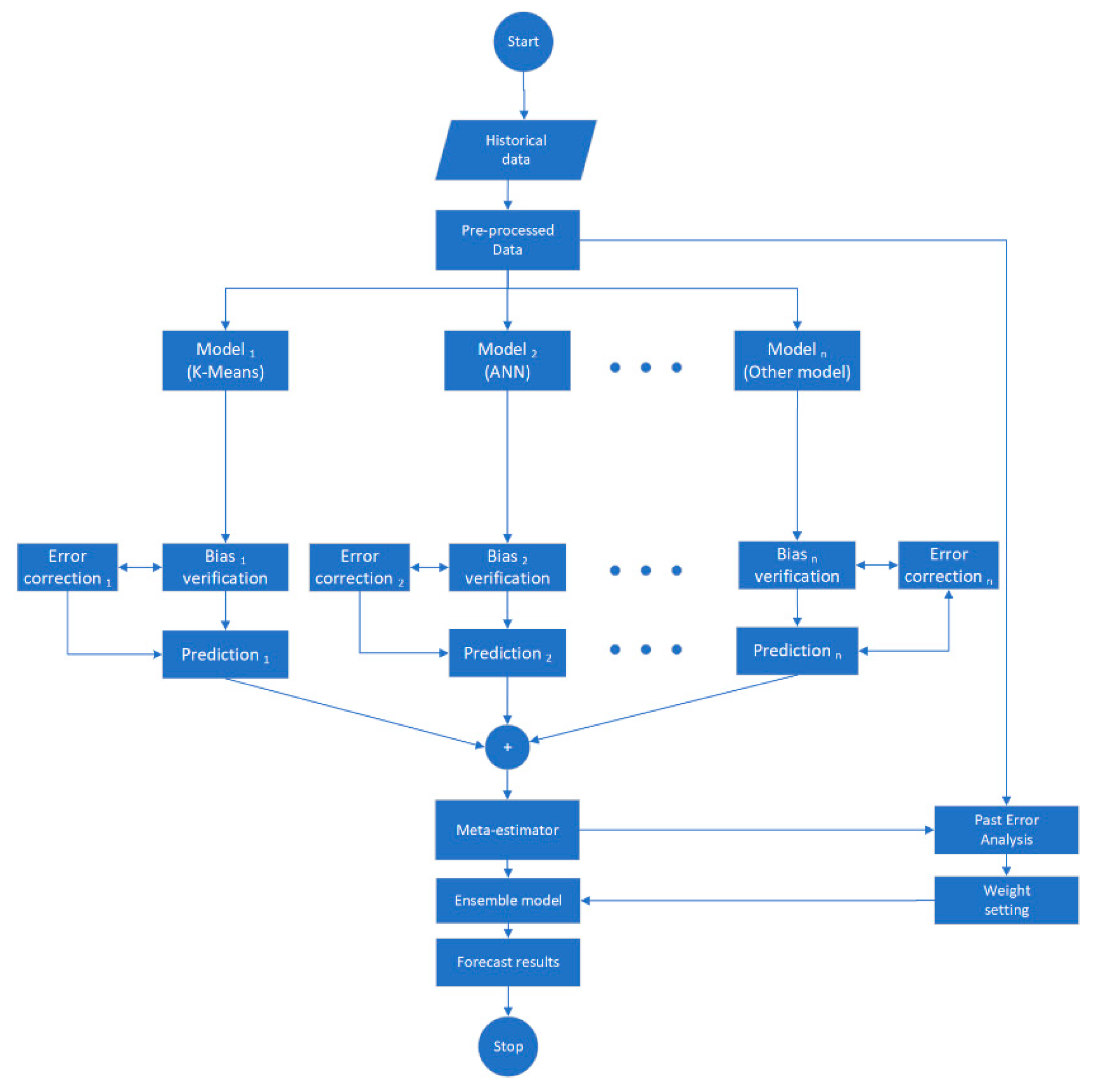
3.3. The Ensemble Strategy of Multiple Models

The predictive ensemble model (PEM) in this study is an adaptation of the random forest algorithm. PEM integrates series of forecasting models to formulate a forecasting model. The integration process is in two stages: optimal weight estimation and stochastic forecast result generation. The optimal weight estimation method estimates the hyperparameters of the parametric predicting models using particle swarm optimization (PSO) at each given time, as defined in Equation (13).

$$f_{e,t}\left(X_{n,t}\right)={\displaystyle \sum }_{n=1}^N{\omega }_{n,t}·f_{n,t}\left(X_{n,t}\right)$$

(13)

The weights $\omega$ are estimated by solving the optimization problem using the heuristic function above and the algorithm in Equation (14), where ${\widehat{\omega }}_T$ and ${\omega }_{n,t}$ is the estimated optimal weight vector for the period T and weight parameter of the n-th model at the time, t, respectively.

$${\widehat{\omega }}_T=\begin{array}{c}argmin\\ {\omega }_T\end{array}{\displaystyle \sum }_{t\in T}{L}_t\left({\displaystyle \sum }_{n=1}^N{\omega }_{n,t}·f_{n,t}\left(X_{n,t}\right),y_t\right)$$

(14)

s.t.

$${\displaystyle \sum }_{n=1}^N{\omega }_{n,t}=1;{\omega }_{n,t}\ge 0 \forall n\in \left\{1,\dots ,N\right\}$$

(15)

The determination of the weights for each model per each forecast instance is initially chosen at random following the set constraints. The weights are subsequently adjusted dynamically as a result of the bias of each point forecast. With the loss function defined to estimate the error associated with each point forecast, the goal of the optimization process is to minimize the loss function, $L_t$, as described in Equation (16), where $X_{n,t}$ and $y_t$ are the input parameter vector of the n-th parametric model and the actual load at time, t, respectively.

$$L_t={\displaystyle \sum }_{n=1}^N\left({\omega }_{n,t}·f_{n,t}\left(X_{n,t}\right)-y_t\right);\forall t\in \left\{1,\cdots ,T\right\}$$

(16)

The weight vector with the minimum loss function becomes the optimal weight vector. Subsequently, the optimal weight estimation is the error estimation distribution with the optimal weight vector. The stochastic forecast results are, therefore, estimated based on the error distribution and the optimal weight vector, as described in Algorithm 1.

Algorithm 1: Algorithm for Stochastic Demand Load Forecast.
Input:	Recent past actual load data
	Forecast period feature parameters
	Estimated ensemble hyperparameters
	Trained prediction models
Output:	Time-series stochastic load forecast
1:	Select the input parameters, $X_{n,t}$ from the set of n forecast features variables at time t.
2:	For each point-forecast model, $f_n$ estimate the load ${\widehat{y}}_t$, at time t with ensemble hyperparameter ${\omega }_{n,t}$ as shown:
	${\widehat{y}}_t={\displaystyle {\displaystyle \sum }_{n=1}^N}{\omega }_{n,t}·f_{n,t}\left(X_{n,t}\right);\forall t\in \left\{1,\cdots ,T\right\},\forall n\in \left\{1,\cdots ,N\right\}$
3:	For each measured load, $y_t$ from a set of recently measured load data, forecast the demand load, $L_t$ and estimate the error, ${\epsilon }_t$ as follows:
	${\epsilon }_t=\left|L_t-y_t\right|$; $\forall t\in \left\{1,\cdots ,T\right\}$
4:	Shift the load forecast, ${\widehat{y}}_t$ with the error ${\epsilon }_t$ as follows:
	${\widehat{y}}_t^{\prime }$ = ${\widehat{y}}_t+{\epsilon }_t$; $\forall t\in \left\{1,\cdots ,T\right\}$
5:	Fit a histogram to ${\widehat{y}}_t^{\prime }$. From the histogram, we estimate the mean, minimum and maximum value at a 95% confidence interval

3.4. Error Correction Model

The predictive framework proposed in this study is designed for short-term and long-term stochastic load forecasts. The framework is based on feature characteristics of historical data. However, the state characteristics of the model features may change because of uncertainties in feature variable predictions or contingencies. Thus, for each parametric model, an error correction model is defined to cater for irregularities with the forecast due to sudden changes in the feature parameters. The error correction model (ECM) is dedicated to estimating the deviations from long-term estimates to influence short-term forecasts. The ECM is defined to compensate for three error types: variance, permanent bias, and temporary bias of the prediction models. Two of the ECMs (i.e., variance and permanent bias) deal with K-means predictions, whereas the temporary bias ECM caters to ANN prediction irregularities.

3.4.1. Variance Error Correction

The traditional K-means algorithm is a vector quantization method that partitions observation into distinctive clusters. Each cluster centroid represents all members in the cluster. However, the centroid representation can lead to a high variance since each demand load profile of the cluster is represented by the same centroid, as shown in Figure 6 and Figure 7. To compensate for such anomalies in the prediction, we defined a correction model, part of the ECM, as described in Algorithm 2, called the variance correction model. With this, the forecasted load profile was adjusted with the mean error of the recent seven-day actual demand load profile forecast. This process alters the forecasted cluster centroid with the deviations with the latest forecast to compensate for maximum variations with each cluster centroid.

Algorithm 2: Variance Error Correction Model.
Input:	Recent past 7-days(N) actual load data
Output:	Deterministic load forecast values
1:	Select the input parameters, $X_{i,t}$ from the set of features variables at time t of load profile, $L_{i\cdots }$
2:	Estimate the load ${\widehat{y}}_{t,i}$, at time t of each daily load profile, $L_i$ with K-means forecast model, $f_t$
	${\widehat{y}}_{t,i}=f_t\left(X_{n,t}\right)$; $\forall t\in \left\{1,\cdots ,T\right\}$, $\forall n\in \left\{1,\cdots ,N\right\}$
	Repeat process; $\forall i\in \left\{1,\cdots ,7\right\}.$
3:	For each actual load, $y_t$ from a set of recent 7-days, measured load data, estimate the error, ${\epsilon }_{t,i}$ as follows:
	${\epsilon }_{t,i}=y_t-{\widehat{y}}_{t,i}$; $\forall t\in \left\{1,\cdots ,T\right\}$, $\forall i\in \left\{1,\cdots ,N\right\}$
4:	For the forecast period, t, estimate average error:
	$\overline{{\epsilon }_t}=\frac{1}{N}{\displaystyle {\displaystyle \sum }_{i=1}^7}{\epsilon }_{t,i}i\in \mathrm{N},\forall t\in \left\{1,\cdots ,T\right\},\forall i\in \left\{1,\cdots ,N\right\}$
5:	Shift load forecast, ${\widehat{y}}_t$ with mean error $\overline{{\epsilon }_t}$ to form shifted load ${\widehat{y}}_t^{\prime }$ as follows:
	${\widehat{y}}_t^{\prime }$=${\widehat{y}}_t+\overline{{\epsilon }_t}$; $\forall t\in \left\{1,\cdots ,T\right\}$

3.4.2. Permanent Bias Error Correction

The demand load profile varies with time, even with a similar set of predictors, as shown in

Table 2. A set of similar load predictors.

Date	P1	P2	P3	P4
23 June 2017	5	4	34.8	1
19 July 2018	4	4	34.7	1

. The prediction gap can be significant, as depicted in Figure 8. These changes are mainly due to the addition of power equipment or changes in the number of users. As mentioned earlier, the information on the feature state characteristics is not accounted for by the K-means model.

A permanent bias error correction model is, therefore, devised to compensate for the variations in the demand load profile. With an intermittent short-term (i.e., 15 min) forecast interval, the correction model uses an estimated error rate of the actual data of the previous seven days to retard the forecast deviation, as shown in Figure 9. The algorithm for this process is described in Algorithm 3. The variance error correction precedes the permanent bias error correction.

Algorithm 3: Permanent Bias Error Correction Model.
Input:	Recent past 7-days(N) actual load data
Output:	Deterministic load forecast values
1:	Select the input parameters, $X_{i,t}$ from the set of features variables at time t of load profile, $L_i$.
2:	Estimate the load ${\widehat{y}}_{t,i}$, at time t of each daily load profile, $L_i$ with K-means forecast model, $f_t$
	${\widehat{y}}_{t,i}=f_t\left(X_{n,t}\right)$; $\forall t\in \left\{1,\cdots ,T\right\}$, $\forall n\in \left\{1,\cdots ,N\right\}$
	Repeat process; $\forall i\in \left\{1,\cdots ,7\right\}.$
3:	For each actual load, $y_t$ from a set of recent 7-days, measured load data, estimate the error, ${\epsilon }_{t,i}$ as follows:
	${\epsilon }_{t,i}=y_t-{\widehat{y}}_{t,i}$; $\forall t\in \left\{1,\cdots ,T\right\}$, $\forall i\in \left\{1,\cdots ,N\right\}$
4:	For the forecast period, t, estimate average error:
	$\overline{{\epsilon }_t}=\frac{1}{N}{\displaystyle {\displaystyle \sum }_{i=1}^7}{\epsilon }_{t,i}$
	$i\in \mathrm{N},\forall t\in \left\{1,\cdots ,T\right\}$, $\forall i\in \left\{1,\cdots ,N\right\}$
5:	For all $t\in \mathrm{T},$ if $\overline{{\epsilon }_t} \nless 0$ or $\overline{{\epsilon }_t} \ngtr 0$, then estimate error rate, ${\epsilon }_r:$
	${\epsilon }_r=\frac{\overline{{\epsilon }_t}}{y_t};t\in \left\{1,\cdots ,T\right\}$, $\forall r\in \left\{1,\cdots ,N\right\}$
6:	Shift load forecast, ${\widehat{y}}_t$ with error rate ${\epsilon }_r$ to form shifted load ${\widehat{y}}_t^{\prime }$ as follows:
	${\widehat{y}}_t^{\prime }=\frac{{\widehat{y}}_t}{1-{\epsilon }_r};t\in \left\{1,\cdots ,T\right\}$, $\forall r\in \left\{1,\cdots ,N\right\}$

3.4.3. Temporary Bias Error Correction

Special event bias may occur with persistent multiple error events even after the application of the error correction models mentioned above, as shown in Figure 10. Special event bias is defined as a sudden change in the amount of power over a quarter of the maximum load happening in a two-or-more-hour period. The evidence of such occurrences is significant in most demand load data. A classic example is the Korean research institute (KEPRI) building demand load data used in our case study analysis. In the dataset, the total number of such occurrences was 91 over a 553-day period.

Although it is sudden, the occurrence of special event bias is significant in a given period. From Figure 11, the duration of the sudden bias is logarithmic in time. The highest magnitude of the bias lasts for the first few hours and monotonically decreases with time to the nominal value. In this study, we compensated for these sudden changes in the demand load forecast with a temporal bias error correction model. The procedure for the error compensation is similar to the permanent bias error correction, except for the required input data and error correction formula. The occurrence distribution and occurrence duration distribution are shown in Figure 12 and Figure 13, respectively.

Actual data for the previous 3 h (T) was utilized to estimate the error for compensation. The formulation of the correction model, as defined in Equation (17), is to correct the average quantum of the special event, learned for one hour until the power remains zero. An initial correction value, $\alpha ,$ is an average of the event values that occurred in the past. With the KEPRI demand dataset, $\alpha$ was estimated as 312.6 KW. Considering that temporary bias error correction is a model for accident events, the average elapsed period, T, was set to be 3.5 h, which is the average time required to identify an event.

$${\widehat{y}}_t=\alpha (1-e^{-\frac{T-t}{t^5}})$$

(17)

4. Case Study and Scenario Analysis

In this section, we show the performance of the proposed framework. In the first part, we test the algorithm on the Korean Electric Power Company (KEPCO) load consumption data from the Korean research institute (KEPRI) building and substation. The load data and weather information used were acquired from iSmart [44] and K-weather [45], respectively. We compare our forecast results with parametric model forecasts. In the second part, we test the algorithm on a set of generalized testbed data of different load sizes, shapes, and characteristics. Smart energy meters and IoT sensors were used to gather load data and feature data for the prediction analysis. Prediction analysis for four seasons—spring, summer, fall, and winter—was conducted in each case study. The optimal values estimated were used to predict randomly selected days for each season. In this study, the average model training computational time and predictive time are specified in

Table 3. The computation time of processes.

Process	Model Training [s]	Forecast [s]
K-means	50.86	1.44
ANN	61.70	20.58
Ensemble	592.75	0.002

. All the data processing and modeling tasks were implemented using MATLAB software (2019a, MathsWorks, Natick, MA, USA) on a 64-bit Intel i7 (4 CPUs and 16 GB RAM) with Windows operating system. The proposed model is relatively computationally non-intensive for both online and offline load forecasts. However, the training computation time could be reduced with parallel processing.

4.1. Case I: Performance of the Proposed Model on Korea Power Company Buildings Dataset

Our predictive analysis, first and foremost, begins with the electrical load dataset from KEPRI building and KEPCO dong-Daegu substation building for which historical data is available from 2015 to date, as shown in Figure 14 and Figure 15 respectively. Based on the available accumulated historical demand load and weather information data, a prediction model was developed. We estimated the prediction accuracy by predicting demand loads of 2019, considering both the MAPE and RMSE indices.

The first stage of the analysis was to analyze the scenarios of two datasets (i.e., KEPRI and KEPCO) of different feature characteristics. These datasets contain demand load and feature data at a 15-minute sample resolution. The datasets cover the period of five years from September 2015. A four-year dataset was used to train the predictive model, whereas a one-year dataset was used for testing and cross-validation. The hyperparameters were tuned to compensate for error correction using the seven days prior to the starting date. Specific days among the four seasons were selected for load prediction. Figure 16 and Figure 17 show the stochastic forecast results of the ensemble prediction for the selected days in each season of the two datasets above.

From the result, it is imperative to know that all seasons take the shape and form of the actual measured load profile. In most cases, the actual measured values lie within the minimum and maximum confidence interval. Before reporting the performance of the ensemble model obtained by combining multiple individual models, we first analyzed the performance of the parametric models mentioned in Section 3. With the same dataset for both training and validation, we estimated the demand load forecast with ANN and K-means separately without the ensemble effect.

To yield credible results, we trained each model multiple times and averaged the losses. From the prediction error results, as shown in Figure 18 and

Table 4. Prediction accuracy of forecasting dataset.

Dataset			Ensemble	K-Means with Bayesian	ANN
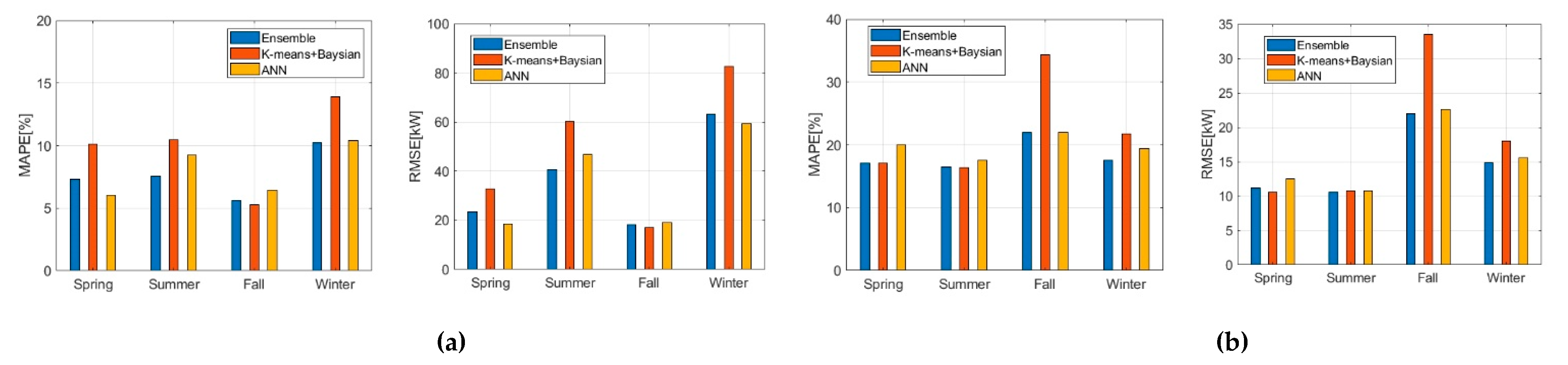
KEPCO dataset	MAPE	Spring	17.0928	17.06893	20.04814
		Summer	16.45506	16.33028	17.51668
		Fall	22.02287	34.34863	21.94459
		Winter	17.57218	21.73072	19.42727
	RMSE	Spring	11.19016	10.59841	12.52269
		Summer	10.55273	10.79871	10.73513
		Fall	22.00363	33.5403	22.5707
		Winter	14.8416	17.97763	15.57768
KEPRI dataset	MAPE	Spring	7.3435	10.1011	6.013
		Summer	7.52238	10.4581	9.22479
		Fall	5.62856	5.27346	6.41714
		Winter	10.2523	13.90402	10.38853
	RMSE	Spring	23.41024	32.69604	18.52118
		Summer	40.75116	60.16406	46.72084
		Fall	18.07842	17.08345	19.13558
		Winter	63.23432	82.75472	59.46993

, it is observed in the figures that the ensemble model can improve the performance of the model, with the error correction model implementation. For simplicity, the ensemble model consisted of only two parametric models, but the framework is scalable for multiple models.

4.2. Case II: Performance of the Proposed Model on Testbed Dataset

The second scenario of the case studies was to examine the adaptability of the proposed model. To this end, we use the hyper-parameters of the ensemble model tuned with the testbed dataset to train load forecasting models for different load form forecasts. Here, the load profile of the dataset does not follow any regular pattern, unlike in Case I. The testbed platform gathers information from a living laboratory, which consists of research laboratories, teaching classrooms, and faculty offices. The activities in these places are not routine; hence, the load profile does not follow a regular pattern, as shown in Figure 19.

For the proposed ensemble model, the training period was from June 2015 to December 2018. Similar to Case I, neural network and K-means parametric models, together with the proposed ensemble model, were used to train demand data independently from 2015 to May 2019, while the data from June 2019 to December 2019 was used for the forecast. Figure 20 and Figure 21 show the results of the stochastic forecast and prediction accuracy, respectively. It is seen in the figures that the proposed ensemble model has the lowest overall MAPE and RMSE among the predictive models.

For all three prediction models, we repeated the trials for randomly selected days and estimated the average MAPE and RMSE. As shown in Figure 21 and

Table 5. Prediction accuracy of forecasting testbed dataset.

Performance Index		Ensemble	K-Means with Bayesian	ANN
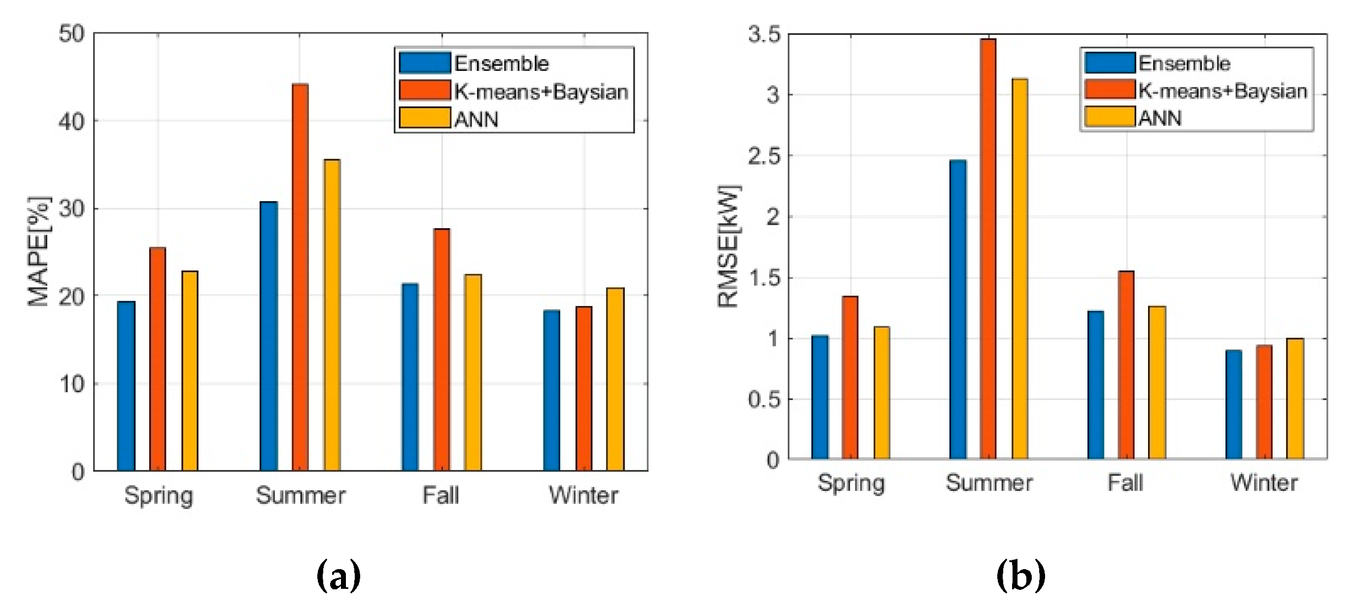
MAPE	Spring	19.27277	25.50984	22.78469
	Summer	30.74737	44.09545	35.52047
	Fall	21.35013	27.61316	22.40761
	Winter	18.30707	18.67867	20.87263
RMSE	Spring	1.01556	1.34224	1.085257
	Summer	2.455532	3.452222	3.130337
	Fall	1.21539	1.541551	1.264588
	Winter	0.892299	0.938574	0.999332

, the ensemble strategy dramatically reduces the losses of MAPE and RMSE, especially for different load profiles with no regular pattern. It is, therefore, reasonable to conclude that the proposed model is robust even for demand load with many irregularities in load patterns. It is also observed that the ensemble strategy can reduce the deviation of multiple trials. This also indicates the higher adaptive capability of the proposed model with the ensemble strategy.

5. Conclusions

This paper proposes an ensemble prediction framework for stochastic demand load forecasting to take advantage of the diversities in forecasting models. The ensemble problem is formulated as a two-stage random forest problem with a series of homogenous prediction models. A heuristic trained model combiner, together with an error correction model, enable the proposed model to have high accuracy as well as satisfactory adaptive capabilities. KEPRI building, KEPCO substation building, and testbed datasets were used to verify the effectiveness of the proposed model with different case scenarios. The comparisons with existing parametric models show that the proposed model is superior in both forecasting accuracy and robustness in load profile variation. The results from the case study analysis show that the proposed ensemble method effectively improves the forecasting performance when compared with individual models. For simplicity, two parametric models(i.e., K-means with Bayesian and ANN models) were adapted in this analysis. However, in future work, other deep learning models, such as a recurrent neural network (RNN) and long short-term memory (LSTM) neural network, can be seamlessly incorporated into the model to enhance its performance.

References

- Spiliotis, K.; Ramos Gutierrez, A.I.; Belmans, R. Demand flexibility versus physical network expansions in distribution grids. Appl. Energy 2016, 182, 613–624. [Google Scholar] [CrossRef]
- Fitariffs. Feed-in Tariffs. Available online: https://www.fitariffs.co.uk/fits/ (accessed on 14 January 2019).
- Nosratabadi, S.M.; Hooshmand, R.-A.; Gholipour, E. A comprehensive review on microgrid and virtual power plant concepts employed for distributed energy resources scheduling in power systems. Renew. Sustain. Energy Rev. 2017, 67, 341–363. [Google Scholar] [CrossRef]
- Fan, C.; Xiao, F.; Wang, S. Development of prediction models for next-day building energy consumption and peak power demand using data mining techniques. Appl. Energy 2014, 127, 1–10. [Google Scholar] [CrossRef]
- Xenos, D.P.; Mohd Noor, I.; Matloubi, M.; Cicciotti, M.; Haugen, T.; Thornhill, N.F. Demand-side management and optimal operation of industrial electricity consumers: An example of an energy-intensive chemical plant. Appl. Energy 2016, 182, 418–433. [Google Scholar] [CrossRef]
- Sepehr, M.; Eghtedaei, R.; Toolabimoghadam, A.; Noorollahi, Y.; Mohammadi, M. Modeling the electrical energy consumption profile for residential buildings in Iran. Sustain. Cities Soc. 2018, 41, 481–489. [Google Scholar] [CrossRef]
- Tucci, M.; Crisostomi, E.; Giunta, G.; Raugi, M. A Multi-Objective Method for Short-Term Load Forecasting in European Countries. IEEE Trans. Power Syst. 2016, 31, 3537–3547. [Google Scholar] [CrossRef]
- Wang, C.-h.; Grozev, G.; Seo, S. Decomposition and statistical analysis for regional electricity demand forecasting. Energy 2012, 41, 313–325. [Google Scholar] [CrossRef]
- Calderón, C.; James, P.; Urquizo, J.; McLoughlin, A. A GIS domestic building framework to estimate energy end-use demand in UK sub-city areas. Energy Build. 2015, 96, 236–250. [Google Scholar] [CrossRef]
- Raza, M.Q.; Khosravi, A. A review on artificial intelligence based load demand forecasting techniques for smart grid and buildings. Renew. Sustain. Energy Rev. 2015, 50, 1352–1372. [Google Scholar] [CrossRef]
- Wang, Q.; Zhou, B.; Li, Z.; Ren, J. Forecasting of short-term load based on fuzzy clustering and improved BP algorithm. In Proceedings of the 2011 International Conference on Electrical and Control Engineering, Yichang, China, 16–18 September 2011; pp. 4519–4522. [Google Scholar]
- Hernandez, L.; Baladron, C.; Aguiar, J.M.; Carro, B.; Sanchez-Esguevillas, A.; Lloret, J.; Chinarro, D.; Gomez-Sanz, J.J.; Cook, D. A multi-agent system architecture for smart grid management and forecasting of energy demand in virtual power plants. IEEE Commun. Mag. 2013, 51, 106–113. [Google Scholar] [CrossRef]
- Hippert, H.S.; Pedreira, C.E.; Souza, R.C. Neural networks for short-term load forecasting: A review and evaluation. IEEE Trans. Power Syst. 2001, 16, 44–55. [Google Scholar] [CrossRef]
- Kaytez, F.; Taplamacioglu, M.C.; Cam, E.; Hardalac, F. Forecasting electricity consumption: A comparison of regression analysis, neural networks and least squares support vector machines. Int. J. Electr. Power Energy Syst. 2015, 67, 431–438. [Google Scholar] [CrossRef]
- Jain, R.K.; Smith, K.M.; Culligan, P.J.; Taylor, J.E. Forecasting energy consumption of multi-family residential buildings using support vector regression: Investigating the impact of temporal and spatial monitoring granularity on performance accuracy. Appl. Energy 2014, 123, 168–178. [Google Scholar] [CrossRef]
- Kuo, R.J.; Li, P.S. Taiwanese export trade forecasting using firefly algorithm based K-means algorithm and SVR with wavelet transform. Comput. Ind. Eng. 2016, 99, 153–161. [Google Scholar] [CrossRef]
- Zhang, F.; Deb, C.; Lee, S.E.; Yang, J.; Shah, K.W. Time series forecasting for building energy consumption using weighted Support Vector Regression with differential evolution optimization technique. Energy Build. 2016, 126, 94–103. [Google Scholar] [CrossRef]
- Massana, J.; Pous, C.; Burgas, L.; Melendez, J.; Colomer, J. Short-term load forecasting for non-residential buildings contrasting artificial occupancy attributes. Energy Build. 2016, 130, 519–531. [Google Scholar] [CrossRef]
- Sandels, C.; Widén, J.; Nordström, L.; Andersson, E. Day-ahead predictions of electricity consumption in a Swedish office building from weather, occupancy, and temporal data. Energy Build. 2015, 108, 279–290. [Google Scholar] [CrossRef]
- Wang, X.; Lee, W.; Huang, H.; Szabados, R.L.; Wang, D.Y.; Olinda, P.V. Factors that Impact the Accuracy of Clustering-Based Load Forecasting. IEEE Trans. Ind. Appl. 2016, 52, 3625–3630. [Google Scholar] [CrossRef]
- Deihimi, A.; Orang, O.; Showkati, H. Short-term electric load and temperature forecasting using wavelet echo state networks with neural reconstruction. Energy 2013, 57, 382–401. [Google Scholar] [CrossRef]
- Mena, R.; Rodrguez, F.; Castilla, M.; Arahal, M. A prediction model based onneural networks for the energy consumption of a bioclimatic building. Energy Build. 2014, 82, 142–155. [Google Scholar] [CrossRef]
- Wang, Y.; Chen, Q.; Sun, M.; Kang, C.; Xia, Q. An Ensemble Forecasting Method for the Aggregated Load With Subprofiles. IEEE Trans. Smart Grid 2018, 9, 3906–3908. [Google Scholar] [CrossRef]
- Wang, Y.; Zhang, N.; Tan, Y.; Hong, T.; Kirschen, D.S.; Kang, C. Combining Probabilistic Load Forecasts. IEEE Trans. Smart Grid 2019, 10, 3664–3674. [Google Scholar] [CrossRef]
- Chen, Y.; Tan, H.; Berardi, U. Day-ahead prediction of hourly electric demand in non-stationary operated commercial buildings: A clustering-based hybrid approach. Energy Build. 2017, 148, 228–237. [Google Scholar] [CrossRef]
- Fumo, N.; Mago, P.; Luck, R. Methodology to estimate building energy consumption using EnergyPlus Benchmark Models. Energy Build. 2010, 42, 2331–2337. [Google Scholar] [CrossRef]
- Ji, Y.; Xu, P.; Ye, Y. HVAC terminal hourly end-use disaggregation in commercial buildings with Fourier series model. Energy Build. 2015, 97, 33–46. [Google Scholar] [CrossRef]
- Bracale, A.; Caramia, P.; Carpinelli, G.; Fazio, A.R.D.; Varilone, P. A Bayesian-Based Approach for a Short-Term Steady-State Forecast of a Smart Grid. IEEE Trans. Smart Grid 2013, 4, 1760–1771. [Google Scholar] [CrossRef]
- Collotta, M.; Pau, G. An Innovative Approach for Forecasting of Energy Requirements to Improve a Smart Home Management System Based on BLE. IEEE Trans. Green Commun. Netw. 2017, 1, 112–120. [Google Scholar] [CrossRef]
- Deng, Z.; Wang, B.; Xu, Y.; Xu, T.; Liu, C.; Zhu, Z. Multi-Scale Convolutional Neural Network With Time-Cognition for Multi-Step Short-Term Load Forecasting. IEEE Access 2019, 7, 88058–88071. [Google Scholar] [CrossRef]
- Ding, N.; Benoit, C.; Foggia, G.; Bésanger, Y.; Wurtz, F. Neural Network-Based Model Design for Short-Term Load Forecast in Distribution Systems. IEEE Trans. Power Syst. 2016, 31, 72–81. [Google Scholar] [CrossRef]
- Han, L.; Peng, Y.; Li, Y.; Yong, B.; Zhou, Q.; Shu, L. Enhanced Deep Networks for Short-Term and Medium-Term Load Forecasting. IEEE Access 2019, 7, 4045–4055. [Google Scholar] [CrossRef]
- Li, R.; Li, F.; Smith, N.D. Multi-Resolution Load Profile Clustering for Smart Metering Data. IEEE Trans. Power Syst. 2016, 31, 4473–4482. [Google Scholar] [CrossRef]
- Motepe, S.; Hasan, A.N.; Stopforth, R. Improving Load Forecasting Process for a Power Distribution Network Using Hybrid AI and Deep Learning Algorithms. IEEE Access 2019, 7, 82584–82598. [Google Scholar] [CrossRef]
- Ouyang, T.; He, Y.; Li, H.; Sun, Z.; Baek, S. Modeling and Forecasting Short-Term Power Load With Copula Model and Deep Belief Network. IEEE Trans. Emerg. Top. Comput. Intell. 2019, 3, 127–136. [Google Scholar] [CrossRef]
- Tang, X.; Dai, Y.; Wang, T.; Chen, Y. Short-term power load forecasting based on multi-layer bidirectional recurrent neural network. IET Gener. Transm. Distrib. 2019, 13, 3847–3854. [Google Scholar] [CrossRef]
- Teixeira, J.; Macedo, S.; Gonçalves, S.; Soares, A.; Inoue, M.; Cañete, P. Hybrid model approach for forecasting electricity demand. CIRED Open Access Proc. J. 2017, 2017, 2316–2319. [Google Scholar] [CrossRef][Green Version]
- Xu, T.; Chiang, H.; Liu, G.; Tan, C. Hierarchical K-means Method for Clustering Large-Scale Advanced Metering Infrastructure Data. IEEE Trans. Power Deliv. 2017, 32, 609–616. [Google Scholar] [CrossRef]
- Zhang, W.; Quan, H.; Srinivasan, D. An Improved Quantile Regression Neural Network for Probabilistic Load Forecasting. IEEE Trans. Smart Grid 2019, 10, 4425–4434. [Google Scholar] [CrossRef]
- Khan, I.; Capozzoli, A.; Corgnati, S.P.; Cerquitelli, T. Fault Detection Analysis of Building Energy Consumption Using Data Mining Techniques. Energy Procedia 2013, 42, 557–566. [Google Scholar] [CrossRef]
- Carsey, V.J.; Wagner, C.G.; Walters, E.E.; Rosner, B.A. Resistant and test based outlier rejection: Effects on Gaussian one- and two-sample inference. Technometrics 1997, 39, 320–330. [Google Scholar] [CrossRef]
- Jovanovic, R.Z.; Sretenovic, A.A.; Zivkovic, B.D. Ensemble of various neural networks for prediction of heating energy consumption. Energy Build. 2015, 94, 189–199. [Google Scholar] [CrossRef]
- Zhang, Y.N.; O’Neill, Z.; Dong, B.; Augenbroe, G. Comparisons of inverse modeling approaches for predicting building energy performance. Build. Environ. 2015, 86, 177–190. [Google Scholar] [CrossRef]
- KEPCO. iSmart-Smart Power Management. Available online: https://pccs.kepco.co.kr/iSmart/ (accessed on 4 August 2017).
- Kweather. Kweather-Total Weather Service Provider. Available online: http://www.kweather.co.kr/main/main.html (accessed on 6 March 2016).