Leveraging Cell Expansion Sensing in State of Charge Estimation: Practical Considerations

Abstract

Measurements such as current and terminal voltage that are typically used to determine the battery’s state of charge (SOC) are augmented with measured force associated with electrode expansion as the lithium intercalates in its structure. The combination of the sensed behavior is shown to improve SOC estimation even for the lithium ion iron phosphate (LFP) chemistry, where the voltage–SOC relation is flat (low slope) making SOC estimation using measured voltage difficult. For the LFP cells, the measured force has a non-monotonic F–SOC relationship. This presents a challenge for estimation as multiple force values can correspond to the same SOC. The traditional linear quadratic estimator can be driven to an incorrect SOC value. To address these difficulties, a novel switching estimation gain is used based on determining the operating region that corresponds to the actual SOC. Moreover, a drift in the measured force associated with a shift of the cell SOC–expansion behavior over time is addressed with a bias estimator for the force signal. The performance of Voltage-based (V) and Voltage and Force-based (V&F) SOC estimation algorithms are then compared and evaluated against a desired $\pm 5\%$ absolute error bound of the SOC using a dynamic stress test current protocol that tests the proposed estimation scheme across wide range of SOC and current rates.

1. Introduction

The primary function of the battery management system (BMS) is to provide an accurate state of charge (SOC) estimation. The SOC represents the amount of charge in ampere-hours (Ah) remaining in a cell divided by its total capacity [1,2]. The BMS traditionally uses current, voltage, and sometimes temperature measurements to estimate the SOC to plan future actions and to prevent over-charging or discharging of cells. Generally, manufacturers provide conservative estimates of remaining energy, since an overestimation of SOC can leave the vehicle stranded. In the case of unmanned air vehicles (UAV), overestimation of SOC might prevent the vehicle from safe landing, since landing maneuvers require very high power, which typically cannot be achieved at very low SOC levels [3]. Underestimating SOC, on the other hand, wastes valuable resources and adds cost and weight to the vehicles, which is critical for robotic platforms.

From the lithium ion batteries, lithium ion iron phosphate (LFP) has been considered for UAV, hybrid electric vehicles (HEV), and electric vehicles (EV) due to their capacity for fast charging, high power capability, and long cycle life [4]. LFP batteries consists of graphite as the negative electrode and lithium iron phosphate (metal oxide) as the positive electrode [5]. Due to the relative flat half-cell potential the positive electrode exerts (also known as the phase-separating cathode active material) [6], the open circuit voltage (OCV) has a relatively flat slope through most of its operating SOC range (10–95%), as shown in Figure 1. The phase transitions in the graphite material correspond to the different voltage plateaus with respect to SOC, as shown in Figure 1a. This makes SOC estimation difficult under noisy environments [7,8] and inexpensive sensing, such as robotic and automotive applications. Previous work has suggested strain or stress (pressure or force) measurements to augment terminal voltage for SOC estimation [9]. Specifically, the graphite in the negative electrode expands when the lithium ions are intercalating into it, and the positive electrode contracts as the lithium ions leave it causing a change of thickness in the components of the battery [10]. This change in thickness causes the battery to swell. Therefore, the overall observed cell swelling is the summation of the swelling from the positive and negative electrodes. When the cells are constrained to a fixed displacement, as typical in automotive packs, the battery swelling results in an increased force on the fixture. This swelling force can be measured using a load cell [9].

The structural changes of this expansion have been studied from the electrode mechanics point of view with respect to strain/OCV coupling [10,11]. The overall volume change of this expansion results in a monotonic function of SOC for a nickel manganese cobalt (NMC) graphite cell [12]. By measuring the force produced by the expansion and including it in the estimation algorithm, improved SOC accuracy can be achieved as compared to voltage based methods [9,13]. The greatest benefits were observed in the 30–50% SOC region, where the voltage slope was relatively flat, but also at the low SOC level, where voltage drops very fast and is challenging to have an accurate model as the battery ages. The change in measured force vs. SOC over many cycles can also inform better estimates of the battery state of health (SOH) [14]. For the LFP-graphite cell studied here, the anode (negative electrode which is graphite) expands during charging but the simultaneous higher contraction rate of the cathode (positive electrode which is LFP) results in a combined cell contraction in the middle SOC range. The overall result is a non-monotonic F–SOC behavior, as shown in Figure 1b. Due to the F–SOC non-monotonicity, SOC estimation based on measured force is challenging since multiple SOC equilibrium points can correspond to the same measured force. Additionally, all mechanical measurements (force, pressure, or displacement) even after calibration exhibit drift associated with small changes in material and a shift in the SOC–expansion behavior as the battery ages. Loss of cyclable lithium causes a shift in capacity and a change in the SOC–expansion behavior of the cell. This capacity loss shifts the stoichiometric ratio associated with lithium concentration in each electrode and hence changes the electrode expansion [15] as a function of lithium intercalation (Coulombs stored) and the measured force/pressure versus SOC as the unknown drift addressed here. Moreover the LFP pouch cells used here are supported by poron sheets [16] between the cells instead of the spacers used in [13]. Thermal expansion of the battery and fixture and viscoelastic response of the compliant poron pad introduces an additional aging and drift factor. Predicting and modeling this aging behavior requires extensive resources and is currently by-passed by estimating this unknown bias as proposed in this article. As can be appreciated, the drift is a general problem of measuring the mechanical behavior (force, pressure, or displacement) of all batteries and it is not just a battery chemistry (LFP)-related issue.

Battery cell balancing is critical to extend the range of battery powered vehicles, the pack operating lifetime, and charge and discharge power limits [17]. To achieve fast and accurate cell balancing, accurate SOC estimation is needed [18]. Voltage-based SOC estimation for the LFP chemistry is particularly challenging since the voltage is relatively flat with respect to SOC. The proposed method improves the SOC estimation using leveraging information about the cell expansion and contraction during charging and discharging. Cell-to-cell variability due to aging, as well as the resulting changes in the measured force, was not investigated, but should be the focus of future research. The influence of cell balancing or imbalanced cells in a module whose force is measured should also be further investigated following the initial work by [19]. Since there would typically be only one force (or strain) measurement in a pack of series connected cell, cell balancing techniques [20] will be of high importance.

In this paper, we demonstrate the improvement in the SOC estimation of LFP batteries by using mechanical in addition to electrical measurements that can be implemented in packs or modules of both hard encased and pouch cells [21]. A novel solution to the multiple equilibrium SOC points is proposed based on the piecewise linear (PWL) F–SOC characteristic approximation that is further used in a switching gain model-based linear quadratic estimator (LQE) design that consists of a combination of force and voltage measurements [22]. Due to the drift that appears in most force measurements, as shown in Figure 2, the SOC may not be accurately estimated. Therefore a bias state is added to the LQE in order to capture the drift in the force measurement due to un-modeled changes in battery swelling or creep of the plastic materials. Experimental validation is also performed on the model-based (LQE) controller design using the combinations of force and voltage measurements during realistic battery electric vehicle usage profiles including the Dynamic Stress Test (DST). The performance of a controller designed with a “perfect” model is compared to one with model mismatch in the OCV and F–SOC PWL fit. The simulated model mismatch captures the typical modeling uncertainties or changes in the cell expansion and open circuit voltage due to aging [23].

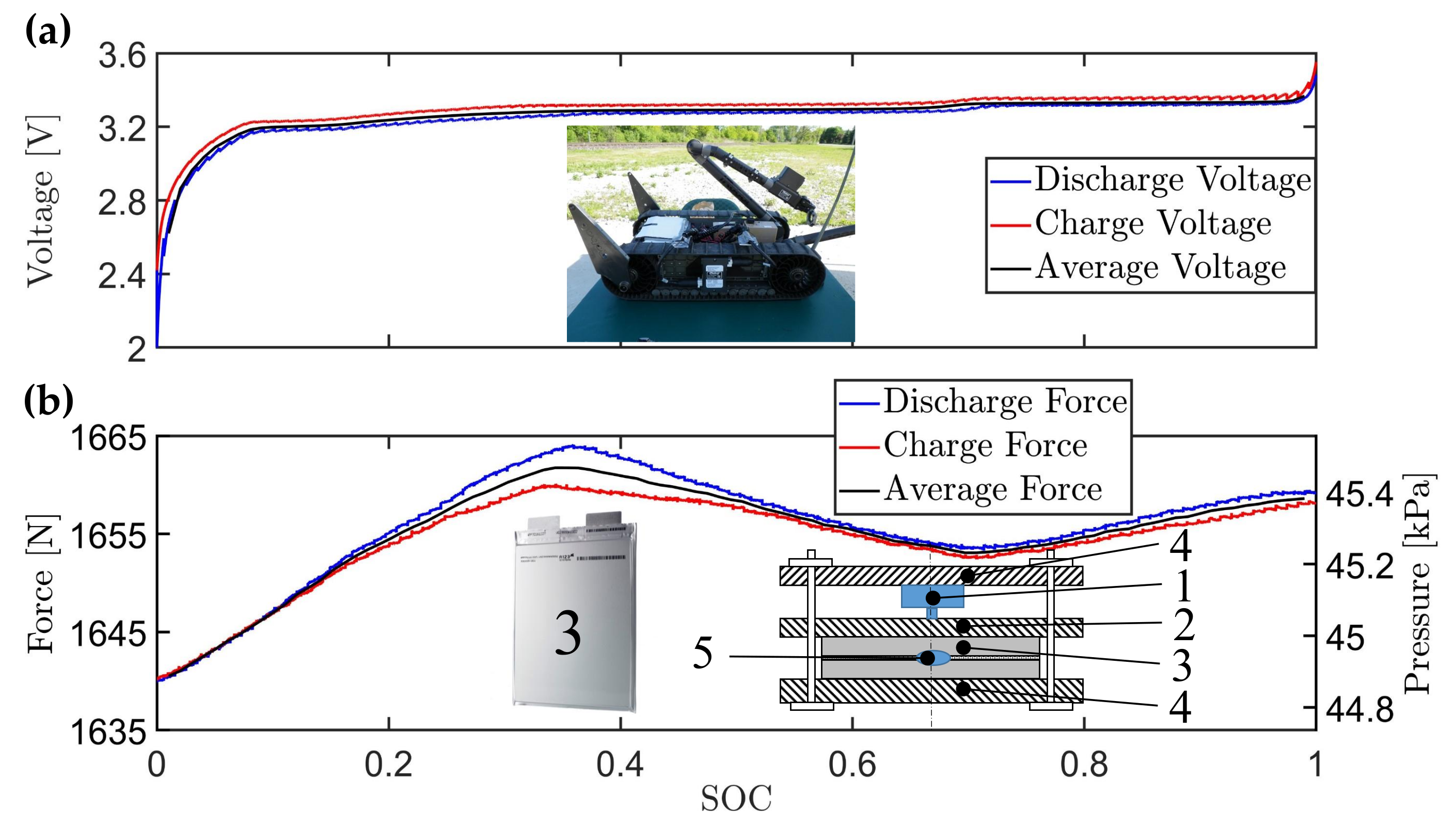
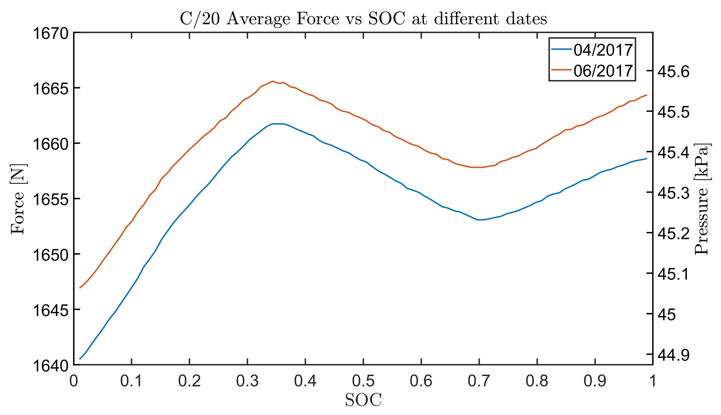
2. Experimental Setup and Force Behavior

The battery considered here for the experimental validation is an A123 20 Ah lithium iron phosphate pouch cell with a voltage range of 3.6–2 V. The fixture, as shown in Figure 1b, consists of an active battery cell (3) (with a temperature sensor on top of it (5)) and a dummy (inactive) cell with a compliant rubber pad in between. The active battery cell and inactive cell consists of a laminated aluminum pouch cell and the rubber pad is a Poron 4701-30 from Rogers, which is 1.14-mm thick. The temperature sensor is a multimeasurand GE sensor that consists of three resistance temperature detectors (RTDs) and one eddy current expansion sensor [21]. The dummy cell and the rubber pad is used as a stress absorber to emulate the conditions a cell might experience in a pack configuration. The purpose of the dummy cell is to simulate the compliance of the whole system. The stiffness of poron is much less than that of the battery, thus the compression of the dummy cell is negligible in terms of the whole system. Therefore, the dummy cell can be used without complicating the force measurement. The dummy cell is held tight by an aluminum bottom end-plate (4), and a movable plate is placed on top of the active cell. This plate has one degree of freedom in the vertical direction with the force sensor (1) placed on top of it. On top of the force sensor, the fixed top aluminum end-plate is bolted to the bottom end-plate to simulate the behavior of a constrained battery pack with fixed distance between the end plates. The force sensor is an Omega (LC305-500) load cell sensor (strain gauge type). The sensor has a 2225 N full scale range with an accuracy of 4.45 N. The load cell and voltage are digitized and recorded by Data Translation DT-9828, which has a voltage accuracy of 2 millivolts. In this paper, the force sensor is used because it is cheaper than the displacement sensors [15], but also less accurate. For example, the accuracy of the displacement sensor used in [15] is 1 $\mathsf{\mu }$m, which corresponds to 0.35 N of compressive force on the poron, while for the Omega force sensor used the accuracy is listed as a percentage of full scale range (4.45 N). The force only accuracy is the important reason for integrating force and voltage information along with performing the bias estimation.

The force plotted against SOC (F–SOC) and the open circuit voltage vs. SOC (OCV–SOC) are measured experimentally using a pulse–relax profile. Specifically, a CCCV charge is applied followed by a pulse–relax discharge profile, with the current rate of $\frac{C}{20}$ for 12 min (which results in a 1% SOC change) followed by a 1 h of rest period to eliminate the influence of the internal resistance and electrolyte polarization of the battery. The data points at the end of the rest are used to obtain the discharge F–SOC and OCV–SOC. The test is then repeated using charge pulses of equal duty cycle. The average between the measurements at the same SOC from the charge and discharge datasets is obtained for the F–SOC, as shown in Figure 1b. The average F–SOC shown in Figure 1b is modeled in Section 3 and is the best fit parameters that match the force inflection points. An average fit is also obtained from data for OCV–SOC and shown in Figure 3a. The values of the fit for the OCV–SOC (average of discharge and charge) and F–SOC can be found in Appendix C.

An important consideration is the drift observed in the measured force between repeated tests as shown in Figure 2. Two average force cycles with an applied current of $\frac{C}{20}$ at different test dates are shown. These cycles have approximately a minimum 3 N and a maximum 6 N of drift in between the second test (performed on 06/2017) and first test (performed on 04/2017). This measurement was taken with the same cell. The drift could be caused by thermal expansion of the battery, pad, and fixture, capacity change or a combination of all four throughout the life of the cell and module on which measurements are performed. That is the reason we have treated the observed bias as an unknown variable. We assume that this unknown/uncertain-origin drift evolves slower than the force measurement from the charge/discharge changes and we therefore can estimate it as an unknown constant bias in real time. This drift in force can affect the SOC estimation if not compensated and, thus, estimation of the sensor bias is used to improve the practical force based SOC estimation.

For the SOC estimation development, tuning, and comparison, two models with two different levels of fidelity are used:

• The simulation model includes the nonlinearities and hysteresis for the electric characteristics detailed in Section 5.
• The observer model ignores hysteresis and uses piecewise linear approximations of the nonlinearities detailed in Section 5.

In the next section, the simulation model is detailed and its efficacy is highlighted in Figure 4 based on a modified DST cycle [24] that is scaled for a 20 Ah Li-ion battery, as shown in Figure 4a. The DST was chosen because it has a current profile that has the combination of the following C-rates and is representative of usage in an electric vehicle: C/4, C/2, 1C, and 2C. If the utilization of the electrode is relatively uniform, the C-rate should not influence the swelling significantly. The electrode expansion depends on the bulk concentration of the electrode solid phase, as opposed to the terminal voltage which depends on the surface concentration [25] and therefore is less sensitive to C-rate. The theory for determining up to what current density the electrode utilization is uniform can be found based on the porous electrode models by Fuller Doyle and Newman [26] and Newman and Tobias [27]. The largest expected contribution of C-rate dependence (or more precisely root mean square (RMS) current) on the result is through thermal expansion of the cell. The experimental profile consists of a Constant-Current/Constant-Voltage (CCCV) charging protocol at a rate of 1C until the battery is fully charged. After a rest period of 30 min, a 1C rate discharge current is applied until it reaches 61% SOC. After the second rest period of 2 h, the modified DST cycle is applied. The resulting voltage, temperature, force, and SOC are shown in Figure 4b–e, respectively. The SOC is calculated by Coulomb counting using a high resolution current sensor and assumed to be the true SOC.

3. Simulation Model

The models described here include the drift present in our force data and higher dynamics such as hysteresis present in our voltage. These models were simulated to validate the robustness of our developed estimators for analysis purposes before the experimental implementation. After this validation, the estimators were used with experimental data and their performance was evaluated. The battery model used for our simulations is presented in the following subsections. The SOC (z) is simply modeled as

$$\frac{dz}{dt}=-\frac{I}{C_b},$$

(1)

where $C_b$ is the cell capacity.

3.1. Cell Swelling Force Model

The force measured at the load cell is modeled using a static non-linearity $F_{sim}\left(z\right)$, which is a function of state of charge, with additive bias and noise terms given by

$$F\left(z\right)=F_{sim}\left(z\right)+v_F+f_d$$

(2)

where $F\left(z\right)$ (N) is the measured force that relies on $F_{sim}\left(z\right)$, which is the PWL model of the average F–SOC behavior; $v_F$ is the measurement noise; and $f_d$ is a constant drift or bias (assumed to be constant but unknown) value present in our force measurement. A piecewise linear representation of the average F–SOC behavior is given by

$$F_{sim}\left(z\right)=C\left(z\right)z+C_0\left(z\right)=\left\{\begin{array}{cc}{\alpha }_{m}z+{\alpha }_{m0},\hfill & \mathrm{if}z\le b_L\hfill \\ {\beta }_{m}z+{\beta }_{m0},\hfill & \mathrm{if}{b}_L<z\le b_H\hfill \\ {\gamma }_{m}z+{\gamma }_{m0},\hfill & \mathrm{otherwise}\hfill \end{array}\right.$$

(3)

where ${\alpha }_m$, ${\beta }_m$, and ${\gamma }_m$ are the slope parameters; ${\alpha }_{m0}$ is the preload or the force sensed at zero state of charge; and $b_L$ and $b_H$ denote the SOC where a change in the sign of the slope in the PWL model occurs as shown by the solid gray vertical lines in Figure 3. These parameter values can be found in Appendix C and can be adjusted to simulate model uncertainty and mismatch. The parameters ${\beta }_{m0}$ and ${\gamma }_{m0}$ in the PWL model are uniquely determined from the other parameters via constraints of piecewise continuity

$${\beta }_{m0}=({\alpha }_m-{\beta }_m)b_L+{\alpha }_{m0}$$

(4)

$${\gamma }_{m0}=({\beta }_m-{\gamma }_m)b_H+({\alpha }_m-{\beta }_m)b_L+{\alpha }_{m0}.$$

(5)

The operating regions R represent the force slope regions determined by our PWL model. The first region is defined as $R_I:\widehat{z}\in [0,{\widehat{b}}_L)$, the second region is defined as $R_{II}:\widehat{z}\in [{\widehat{b}}_L,{\widehat{b}}_H]$, and the third region is defined as $R_{III}:\widehat{z}\in ({\widehat{b}}_H,1]$. The operating regions are shown in Figure 3.

3.2. Terminal Voltage Model

The terminal voltage in volts is modeled as

$$V_T=V_{oc}\left(z\right)-IR-V_1-V_2-V_h+v_V,$$

(6)

where $R\left[\mathsf{\Omega }\right]$ is the total equivalent series resistance, I is the discharge current applied to the battery, $V_1$ and $V_2$ are the voltages due to the two resistance and capacitance (RC) pairs, and $v_V$ represents the V measurement noise. The OCV characteristic, $V_{oc}\left(z\right)$, is SOC dependent and modeled using

$$V_{oc}\left(z\right)=V_0+d(1-exp(-fz))+h\left(1-exp\left(-\frac{-k}{1-z}\right)\right)+gz+\sum _{i=1}^3{a}_{v,i}arctan\left(-\frac{z-b_{v,i}}{c_{v,i}}\right),$$

(7)

where $V_0$, g, d, f, h, k, $a_{v,i}$, $b_{v,i}$, and $c_{v,i}$ are tuned parameters found in Appendix C. The electric equivalent circuit (EC) battery model [28,29] is used for the simulation in our observer validation. In this study, voltage hysteresis ($V_h$) [30] is also considered for the simulation model

$$\frac{d{V}_1}{dt}=\frac{-V_1}{R_1{C}_1}+\frac{I}{C_1}$$

(8)

$$\frac{d{V}_2}{dt}=\frac{-V_2}{R_2{C}_2}+\frac{I}{C_2}$$

(9)

$$\frac{dz}{dt}=-\frac{I}{C_b}$$

(10)

$$\frac{d{V}_h}{dt}=-\left|\frac{{\gamma }_{h}I}{C_b}\right|V_h+\left|\frac{{\gamma }_{h}I}{C_b}\right|H(z,sgn\left(I\right))$$

(11)

where $V_1$ and $V_2$ are the voltages of the RC equivalent circuits, $R_1$ and $R_2$ are the resistors, $C_1$ and $C_2$ are the capacitors of the RC equivalent circuits, $V_h$ is the hysteresis voltage, ${\gamma }_h$ is the hysteresis rate constant, and $H(z,sgn(I\left)\right)$ is a function of SOC and the sign of current ($sgn\left(I\right)$) following [30]. The function $H(z,sgn(I\left)\right)$ is taken to be half the difference between the charge and discharge OCV measurements, and the parameter values can be found in Appendix A. Although the EC model parameters depend on the battery’s SOC and temperature, in this paper, we do not take this dependency into consideration. The constant parameters of the EC model can be found in

Table 1. Battery Equivalent Circuit Parameters and its values.

Parameters	Values
R	1.5 mohms
$R_1$	1.4 mohms
$C_1$	13,014 farad
$R_2$	2.7 mohms
$C_2$	143,000 farad
${\gamma }_h$	0.00054

. The dynamic equations developed for charge/discharge as well as the measurements in Equations (2) and (6) is used to simulate the battery behavior, and it is numerically discretized with a time step of $T_s=1$ s.

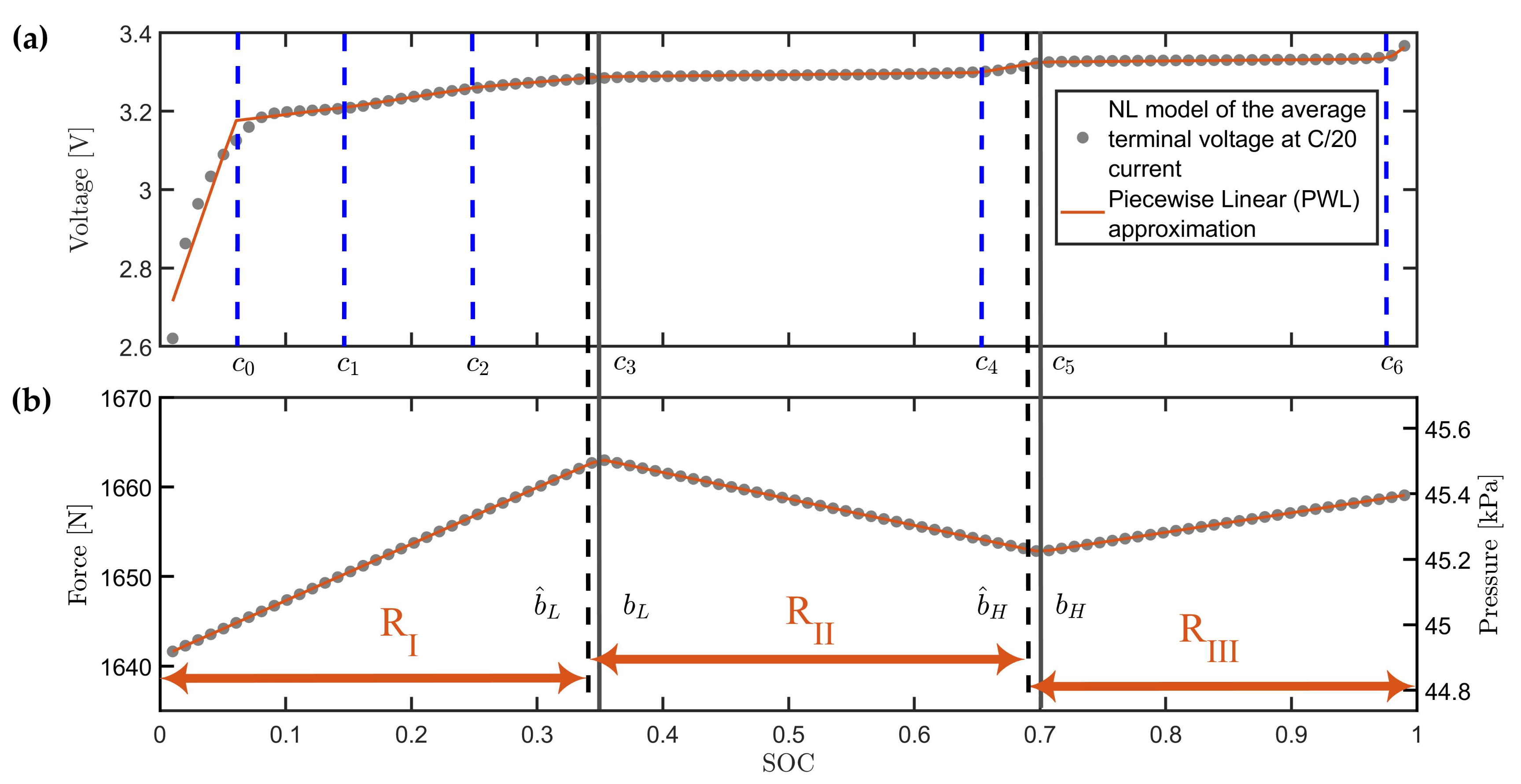
4. Voltage Model Parameterization

Before using our model for SOC estimation, the average Force–SOC and OCV–SOC needs to be obtained and model parameterization of the equivalent circuit parameters is required using a pulsed current profile such as the Hybrid Pulse Power Characterization (HPPC) [28]. The pulse current was obtained and the nonlinear programming solver fmincon was used to find the parameters provided in Table 1. To verify that the parameters are correct, different initialization values were used. From the different initialization values used, fmincon converged to the parameters provided in Table 1.

5. SOC Estimation Model

The linear quadratic estimator (LQE) also known as the steady-state Kalman filter is used for state estimation. The goal of the observer is to find a gain K that converges the initial state to the true state of the system using linear filter equation with measurement error feedback

$${\widehat{x}}_{t+1}=A{\widehat{x}}_t+B{u}_t+K(y_t-{\widehat{y}}_t)$$

(12)

where the estimated output equation is given by

$${\widehat{y}}_t=C\left({\widehat{x}}_t\right){\widehat{x}}_t-C_0\left({\widehat{x}}_t\right)-D{u}_t$$

(13)

with $C\left({\widehat{x}}_t\right)$ the slope of the estimated measurement and $C_0\left({\widehat{x}}_t\right)$ the affine parameter based on our model and shown in Figure 3. The matrix D is the direct transition (or feedthrough) term. The error dynamics are governed by the eigenvalues of $A-KC$, which depends on the chosen gain K so that it is stable and achieves fast convergence of the SOC estimation error $e=z-\widehat{z}$. We use the Discrete Algebraic Riccati Equation (DARE) to find our gain K on all our developed observers. The DARE is defined as

$$P=AP{A}^T-AP{C}^T{\left[CP{C}^T+R\right]}^{-1}CP{A}^T+Q$$

(14)

and solved for the estimation error covariance matrix P. In this equation, Q is the process noise covariance matrix (size $nxn$) and $R\in {\mathbb{R}}^{n_y}$ is the measurement noise covariance matrix (size $mxm$). The values of the diagonal elements of R are chosen based on actual sensor measurement noise variance and Q is tuned so that the desired transient is achieved. The solution of the estimation error covariance (P) for the Kalman filter converges to the solution of Equation (14) for $t\to \infty$ if $(A,C)$ is detectable. In this case, the asymptotically stable observer gain is then computed [31] as

$$K={\left[CP{C}^T+R\right]}^{-1}CPA.$$

(15)

5.1. Voltage Only Observer Design

In the case of voltage only estimation, we neglect the hysteresis dynamic term. This represents a typical model mismatch in voltage measurements. The states of the observer are ${\widehat{x}}_t={[{\widehat{V}}_1,{\widehat{V}}_2,\widehat{z}]}^T$ given by the discretized version of Equations (8)–(10) and the PWL approximation of the nonlinearities in voltage measurement ${\widehat{y}}_t$ is given by the equations in Appendix B. The values of the parameters in the voltage and force models can be found in Appendix C. The gain K for this observer is given as

$$K_V={\left[\begin{array}{ccc}{K}_1& K_2& K_3\end{array}\right]}^T$$

(16)

The values for the gains $K_i$ with $i=$ 1–3 are obtained by tuning the Q matrix. The gain $K_V$ is found for the eight regions in which the voltage is divided: $R_1$: $z\in [0,c_0]$, $R_2$: $z\in (c_0,c_1]$, $R_3$: $z\in (c_1,c_2]$, $R_4$: $z\in (c_2,c_3]$, $R_5$: $z\in (c_3,c_4]$, $R_6$: $z\in (c_4,c_5]$, $R_7$: $z\in (c_5,c_6]$, and $R_8$: $z\in (c_6,1]$.

The main challenge in this system is the slow convergence of the estimation error due to the almost zero output gain (in C) especially the C(1,3) that corresponds to the $\frac{dV}{dz}$ in Equation (18). Increasing the $K_v$ gain to compensate for the low state to output gain C governed by $\frac{dV}{dz}$ will amplify voltage sensor noise. Therefore, another observer is developed that uses voltage and force measurement since SOC and bias in the force signal are unobservable by force measurement only.

5.2. Voltage and Force Observer Design

In the case of force and voltage estimation, the states of the observer are ${\widehat{x}}_t={[{\widehat{V}}_1,{\widehat{V}}_2,\widehat{z}]}^T$ and $\widehat{y}={[{\widehat{V}}_T,\widehat{F}]}^T$ given by the equations in Appendix B. The gains for the V&F observer have the following format

$$K_{VF}={\left[\begin{array}{ccc}{K}_{11}& K_{21}& K_{31}\\ K_{12}& K_{22}& K_{32}\end{array}\right]}^T$$

(17)

and the gain $K_{VF}$ is found for the eight regions of the voltage, as explained in the previous subsection. The modeled force used for the state estimator, $\widehat{F}$, is given by

$${\widehat{F}}_{sim}\left(\widehat{z}\right)={\widehat{C}}_{dF}\left(\widehat{z}\right)\widehat{z}+{\widehat{C}}_0\left(\widehat{z}\right)=\left\{\begin{array}{cc}{\alpha }_m\widehat{z}+{\alpha }_{m0},\hfill & \mathrm{if}\widehat{z}\le {\widehat{b}}_L\hfill \\ {\beta }_m\widehat{z}+{\beta }_{m0},\hfill & \mathrm{if}{\widehat{b}}_L<\widehat{z}\le {\widehat{b}}_H\hfill \\ {\gamma }_m\widehat{z}+{\gamma }_{m0},\hfill & \mathrm{otherwise}\hfill \end{array}\right.$$

(18)

where $\widehat{z}$ is the estimated SOC from our observer and ${\widehat{b}}_L$ and ${\widehat{b}}_H$ are the inflection points that are shifted by −10%, as shown by the dashed black lines in Figure 3 to emulate model uncertainty and aging. In the case of a “perfect” model, ${\widehat{b}}_L=b_L$ and ${\widehat{b}}_H=b_H$.

Switching Logic in Observer Design

The gain (K) of the LQE depends on the relationship between the estimated state and the slope of the measurement. In the case of a monotonic function, the estimated state will converge to the true state value when the estimator gain is chosen so that the error dynamics are stable. In the case of a non-monotonic function, the estimated state and the true state can have different slopes in the force output depending on the operating region. Therefore, the estimator gain would have a wrong sign which would lead to the divergence of the estimated state of charge from the true state. This is due to the traditional LQE using the modeled slope at the region of the estimated state. For example, consider the case where the model initialization occurs in the middle section of the SOC range (force decreases and cell contracts as SOC increases), whereas the actual SOC is in the high SOC range (force increases and cell swells as SOC increases); the traditional approach will lead to divergence of the estimated SOC state from the actual SOC due to the difference in slope. To address this difficulty, an algorithm was developed that uses a window of past measurements force data to identify the slope of the non-monotonic F–SOC. The observer gain will need to switch based on a judicious combination of the information at hand, namely

(a)

the modeled slope ${\widehat{C}}_{dF}$ from Equation (18) of the F–SOC relation based on the estimated state $\widehat{z}$; and

(b)

the estimation of the slope by using the measured force with respect to the Coulomb counting based SOC, $\frac{d\tilde{F}}{dz}$ (DFDZ).

Therefore, the output error injection gain K is a function of the state estimate and the estimated force derivative, e.g., $K(\widehat{z}$, $\widetilde{\frac{dF}{dz}})$, using two sources of information due to its importance in the convergence of the estimation error. The DFDZ is computed as a line fitting problem based on the moving window of past force measurements and the Coulomb counting based SOC integration ($\tilde{z}$) over the moving window. The fitted DFDZ line $\tilde{F}=\frac{d\tilde{F}}{dz}\tilde{z}+{\tilde{F}}_0$ parameters are computed using the least-squares estimation as

$$\begin{array}{c}\hfill {\left[\begin{array}{c}\frac{d\tilde{F}}{dz}\\ {\tilde{F}}_0\end{array}\right]}_k\end{array}={\left({\mathbb{L}}_k^T{\mathbb{L}}_k\right)}^{-1}{\mathbb{L}}_k^T{\mathbb{F}}_k$$

(19)

where ${\tilde{F}}_0$ is the affine parameter in Equation (18). The moving window of force measurements and the design matrix respectively are defined as follows

$$\begin{array}{cc}\hfill {\mathbb{F}}_k=\left[\begin{array}{c}{F}_{k-n}\\ F_{k-n+1}\\ ⋮\\ F_k\end{array}\right],& {\mathbb{L}}_k=\left[\begin{array}{cc}{\tilde{z}}_{k-n}& 1\\ {\tilde{z}}_{k-n+1}& 1\\ ⋮& ⋮\\ {\tilde{z}}_k& 1\end{array}\right]\end{array}$$

(20)

where k represents the discrete-time measurement index and n is the number of past samples. The Coulomb counting based SOC integration is computed as

$${\tilde{z}}_k={\tilde{z}}_{k-1}-\frac{I_{k-1}{T}_s}{C_b}.$$

(21)

The integration is initialized with ${\tilde{z}}_{k-n}=0$. The moving window provides the $\frac{d\tilde{F}}{dz}$ computation as the average slope in a window of n prior values of force which causes a delay $\delta$ in the switching logic as a function of the window size n, as shown in Figure 5d. We can see that for $n=150$ the $\delta$ is smaller compared to $n=450$, but, with smaller n, the estimated slope is more susceptible to noise. We chose n here to be 150 samples with a discretized time of 1 s. The reasoning behind choosing this window size is explained in Section 5.3. Due to this delay and the fact that during this time the actual and the estimated state can be in different segments of the SOC, which could cause divergence, the gain is set to zero when the estimated slope $\frac{d\tilde{F}}{dz}$ has a different sign from the modeled slope. Therefore, the system will run open loop for both voltage and force when there is slope mismatch. This is done in order to avoid instability issues.

The switching logic for our gain ($K(\widehat{z}$,$\widehat{\frac{dF}{dz}})$) is given by the following rules:

$$K_{VF}(3,2)=\left\{\begin{array}{cc}{K}_{R_I}\hfill & \mathrm{if}\frac{d\tilde{F}}{dz}>0and\widehat{z}<{\widehat{b}}_L\hfill \\ K_{R_{II}}\hfill & \mathrm{if}\frac{d\tilde{F}}{dz}<0and{\widehat{b}}_L<\widehat{z}<{\widehat{b}}_H\hfill \\ K_{R_{III}}\hfill & \mathrm{if}\frac{d\tilde{F}}{dz}>0and\widehat{z}>{\widehat{b}}_H\hfill \\ 0\hfill & \mathrm{otherwise}.\hfill \end{array}\right.$$

(22)

Note that the gains $K_{R_I}$, $K_{R_{II}}$, and $K_{R_{III}}$ are not constant. The set of gains $K_{R_I}$ consists of the four gains that correspond to the four regions in voltage in region $R_I$, $K_{R_{II}}$ consists of the two gains that correspond to the two regions in voltage in region $R_{II}$, and $K_{R_{III}}$ consists of the two gains that correspond to the two regions in voltage in region $R_{III}$, as shown in Figure 3. The gains are therefore a function of $\widehat{z}$ and $\frac{d\tilde{F}}{dz}$ and they switch to the corresponding region depending on the value of the estimated slope and estimated SOC.

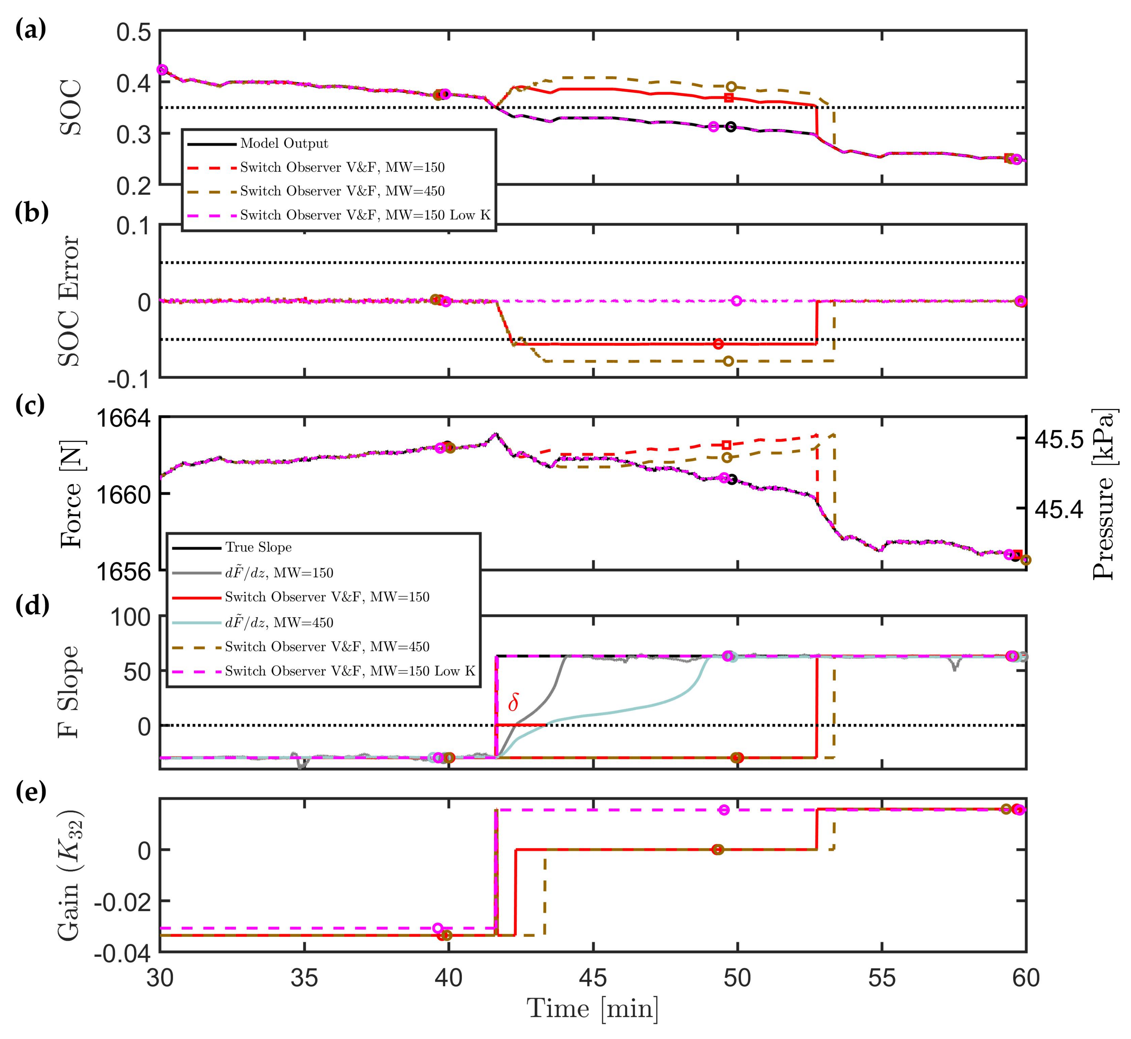
5.3. SOC Estimation Error during Switching

Going open loop, during the time interval when there is a slope mismatch, is not sufficient to avoid divergence of the estimated state of charge with high feedback gain. To verify this, we analyze the Luenberger Observer for the SOC state using the measured force only. The goal of this analysis is to determine the impact of the gain K on divergence of the state estimate when the true model and state estimate are operating on opposite regions of the output non-linearity. Using Equations (12) and (13), we can write the error dynamic ($e=z-{\widehat{z}}_t$) for the observer assuming $\widehat{x}$ is in $R_I$ and x is in $R_{II}$ as:

$${\widehat{e}}_{t+1}=A{\widehat{e}}_t-K(y_t-{\widehat{y}}_t)=A{\widehat{e}}_t-K({\beta }_{m}x+{\beta }_{m0}-{\alpha }_m\widehat{x}-{\alpha }_{m0}+{\alpha }_{m}x-{\alpha }_{m}x)$$

(23)

$${\widehat{e}}_{t+1}=(A-K{\alpha }_m){\widehat{e}}_t-K(({\beta }_m-{\alpha }_m)x+{\beta }_{m0}-{\alpha }_{m0}).$$

(24)

From this error dynamic equation, we notice the error converges to a non-zero quantity so that e tends toward zero only when $x=b_L$, and the steady state error $e_{ss}=(({\beta }_m-{\alpha }_m)x+{\beta }_{m0}-{\alpha }_{m0})/{\alpha }_m$ is independent of the gain K. In the case, where the sign of the model is updated based on the measured slope of the force signal ($\widetilde{\frac{dF}{dz}})$, the growth in SOC estimation error is bounded by the number of samples in the filter or the moving window size ($MW$). If the current is bounded (which it is in our case), then the divergence in the state estimate is bounded by the integral of the current and the switching time $\delta$. When the estimator model is updated to the correct slope, the observer begins to converge again. However, noise in the measurement of force could still result in divergence of the estimate if the gain K is too high. This is shown in Figure 5. We can see that just by changing the $MW=150$ to $MW=450$ by using the same gains given by $Q=diag\left(\right[2,0.1,0.1\left]\right)$ and $R=diag\left(\right[1,1\left]\right)$. This is because the gain is large and the delay in $\frac{d\tilde{F}}{dz}$ crossing zero is 1 min greater than $MW=150$. Therefore, the divergence in SOC, because of the slope mismatch, will grow for a longer period of time with increasing filter length and a higher error is achieved due to the delay in switching the gain to zero.

Now, if we decrease the gain by using $Q=diag$([2,0.1,1 × 10${}^{-2}$]) and $R=diag\left(\right[1,1\left]\right)$ without bias estimation and $n=150$, we notice that at the same region the error decreases by 5%. Therefore, low gains should be used to avoid the divergence and a window size of 150 is chosen since this is the lowest window that provides sufficient noise rejection. The previous error dynamic analysis can be done for the other mismatch slope areas to determine the minimum SOC state estimation error.

5.4. Bias Influence in SOC Estimation

In this section, the proposed estimation is tested under biased force measurements. In Figure 6, the simulated force data have a bias or drift of 3 N present in the force measurement. This drift in force affects the SOC estimation, as shown in Figure 6. Application of the switched model observer based on voltage and the force measurements based on previous work [22] without taking into account the bias estimation results in error larger than $5\%$. Therefore, we assumed a constant bias state (${\widehat{f}}_{d,t}$) that is given by

$$f_{d,t+1}=f_{d,t}$$

(25)

where $f_{d,t}$ is the constant bias or drift term that augments the electrical states. The estimator now estimated the electrical states (except hysteresis) and the force drift with ${\widehat{x}}_t={[{\widehat{V}}_1,{\widehat{V}}_2,\widehat{z},{\widehat{f}}_{d,t}]}^T$. Therefore, the gains for the V&F Bias observer have the following format

$$K={\left[\begin{array}{cccc}{K}_{11}& K_{21}& K_{31}& K_{14}\\ K_{12}& K_{22}& K_{32}& K_{24}\end{array}\right]}^T$$

(26)

The values for $K_{1i}$ and $K_{2i}$ with $i=$ 1–4 are obtained by tuning the Q and R matrices.

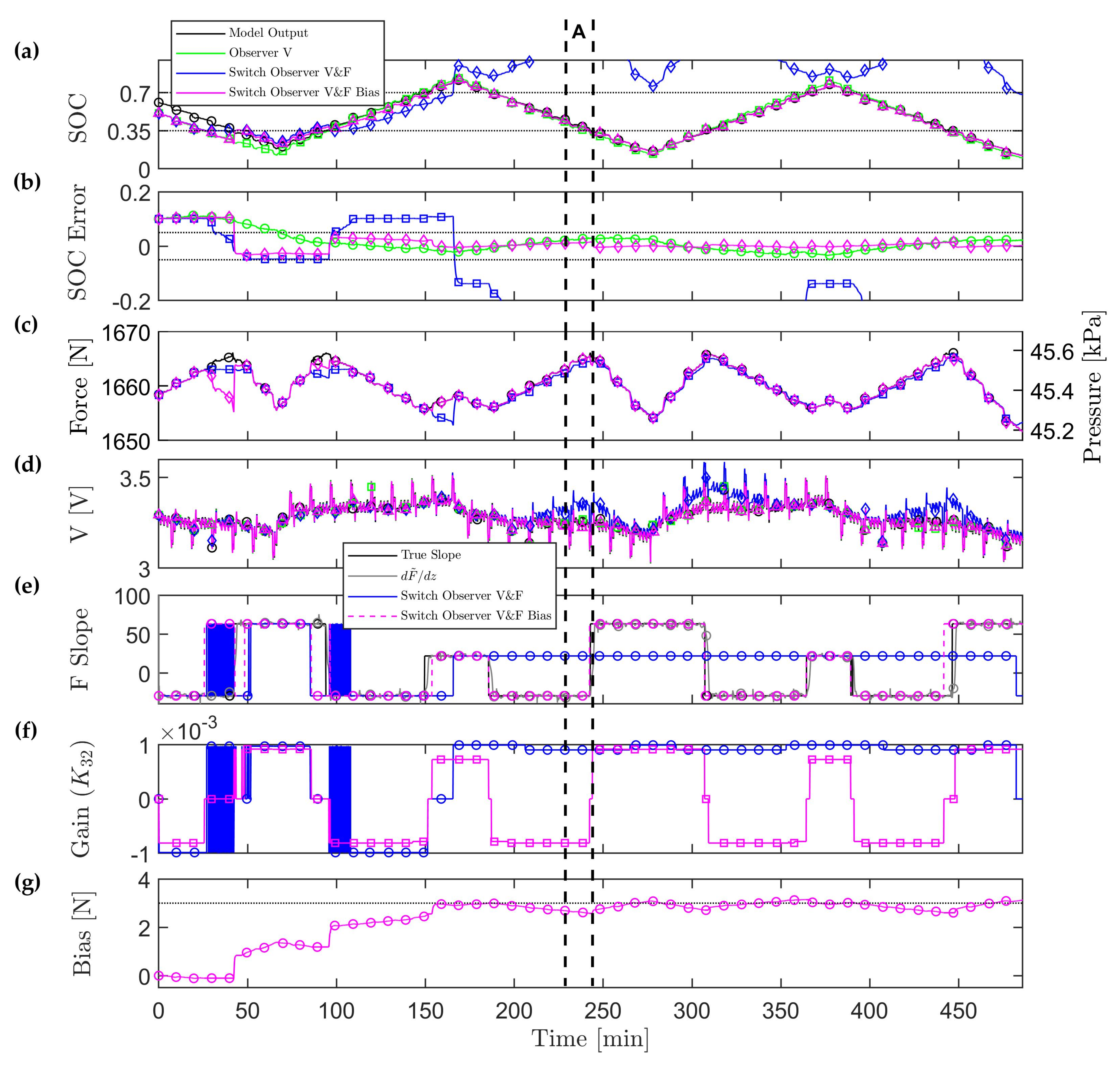
6. Simulation Results without Model Mismatch in F–SOC and OCV–SOC

The standard Dynamic Stress Test (DST) profile is repeated back to back and modified by adding a constant current to periodically recharge the battery at 1/6 C rate, exercising a wider range of SOC, as shown in Figure 4a. A measurement noise variance of 5 mV for voltage and 0.05 N for force was chosen based on the variance of the experimental data. As for the drift value, we chose a value of 3 N based on the monthly drift observed between repeated characterization experiments. Our observer works if the initial error in bias is within 3 N. The LQE estimator is initialized with an SOC error of $\pm 10\%$ in order to evaluate convergence. In the case of the DST cycle, the true SOC state may be approaching the estimated value or diverging from the true SOC value depending on the initial SOC estimation error. The objective is to stay within the $\pm 5\%$ estimation error bound (EEB) for SOC denoted by the dashed lines in the Figure 6b. We chose to simulate initial conditions around 60–80% and the SOC swing of the whole cycle around 20–80% SOC. This range was chosen due to the challenge associated with flat OCV–SOC profile present for voltage (around 40–60%) and the negative slope in F–SOC (around 35–70%). Therefore, the simulated “measured” data are initialized at 61% SOC. The weights chosen to obtain the gains $K_{1i}$ with $i=$ 1–4 and $K_{2i}$ with $i=$ 1–4 are shown in

Table 2. Control weights for the different sensors using the simulated data. V, terminal voltage; V&F, fusion of both sensors; V&F Bias, fusion of both sensors with bias state.

Models	Q	R
V	$diag(2,10,2)$	50
V&F	$diag(2,0.01,0.01)$	diag(50,10,000)
V&F Bias	$diag(2,0.1,0.01,4)$	diag(50,10,000)

. The gain $K_{32}$ is shown in Figure 6f to illustrate when the algorithm uses the estimated slope mismatch to zero the observer gain and run open loop.

The SOC estimation using the V measurement and V&F measurement with and without the bias state estimation are shown in Figure 6a. In all three cases, a $10\%$ initial estimation error is assumed. The inflection points in the force with respect to SOC are denoted by the dotted horizontal lines in Figure 6a. In this case, the correct values for $b_L$ and $b_H$ are used for the simulated data and the observer. The switched model applies zero gain (as shown in Figure 6f in Region A) when the model slope (based on $\widehat{z}$) does not agree with the estimated slope using the least squares on the moving window with Equations (19) and (20). Using the previously developed V&F observer without bias estimation [22], the SOC error does not remain within the $\pm 5\%$ bound with a 3 N bias in the measurement, even though the error in the force signal is small, as shown in Figure 6a,c. For the proposed switching force-and voltage-based LQE with bias (Switch Observer V&F Bias) before $t=50$ min there is an SOC estimation error of 10%, even though the force estimation is matching our simulated data, due the error in bias state estimation shown in Figure 6g. Between $t=25$ and $t=42$ min, there is a slope mismatch in $\frac{d\tilde{F}}{dz}$ due to the delay of our moving window. After $t=42$ min, the slopes match again, and the correct non-zero feedback gain is applied and the state of charge estimation error convergences within our $\pm 5\%$ EEB, as shown in Figure 6b. Even though both the proposed switching force and voltage based LQE (Switch Observer V&F Bias) and the LQE based on voltage (Observer V) estimate voltage accurately (as shown in Figure 6d, it can be observed that the Switch Observer V&F Bias has faster convergence than the estimate based on V alone, as shown in Figure 6b. The faster convergence is due to the addition of the force signal that produces a lower output error injection gain from V to SOC in the regions where the voltage signal has flat slope. It can be appreciated from Figure 6g that the bias term is able to estimate the drift value slowly in our force measurement. The slow convergence of the bias estimate to the 3 N value denoted by the dotted black line can be seen in Figure 6g. Therefore, as time progresses, the estimated force converges to the modeled data, as shown in Figure 6c. This is due to the chosen inflection points in F–SOC function being the same as the modeled data (${\widehat{b}}_L=b_L=c_3$ and ${\widehat{b}}_H=b_H=c_5$). We can observe that the estimated bias value oscillates around the true bias value. The model error is being attributed to the bias state by the estimation algorithm. The Switch Observer V&F Bias has lower root mean square error (RMSE), faster time convergence to the denoted SOC EEB (referred to as Time to 5% EEB in

Table 3. Comparison of the RMSE index for different initial estimate error and different sensors using the simulated data. V, terminal voltage; V&F Bias, fusion of both sensors with bias state.

Initial SOC Error	Parameters	Observer V	Switch Observer V&F Bias
+10%	Time to 5% EEB [min]	67.81	42.44
	Max SOC Error [%]	3.32	3.22
	RMSE	0.0394	0.0337
−10%	Time to 5% EEB [min]	41.33	7.86
	Max SOC Error [%]	5.15	1.54
	RMSE	0.0321	0.0185

), and reduced maximum absolute SOC error after the force measurement has converged to an SOC error (referred to as Max SOC Error in Table 3) compared to Observer V as shown in Table 3. Therefore, the advantage of Switch Observer V&F Bias is the fast convergence in the region of 40–60% SOC while having more accurate SOC estimation due to the low RMSE values.

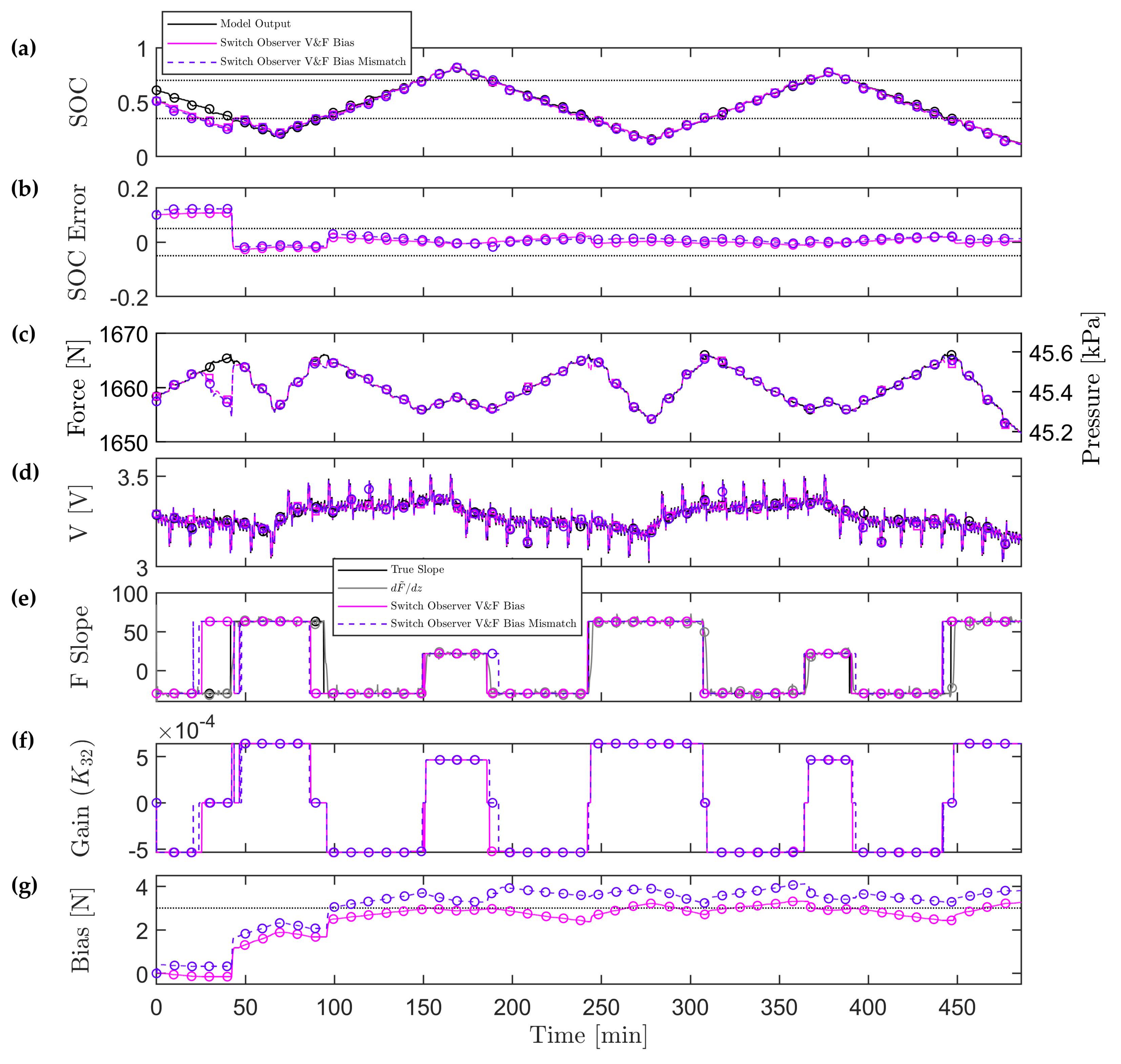
7. Simulation Results with Inflection Point Mismatch in F–SOC and OCV–SOC

In reality, we do not have a “perfect” model that captures the battery data. Moreover, during aging, the capacity loss shifts the inflection points as compared with the fresh cell. Therefore, to simulate a more realistic application model mismatch is included in the F–SOC and OCV–SOC observer by shifting the inflections points $b_L$ and $b_H$ of by −10% (${\widehat{b}}_L$ and ${\widehat{b}}_H$) to represent capacity loss on the negative electrode [15]. During capacity loss, these inflections points shift for both functions of F–SOC and OCV–SOC because they correspond to the electrochemical and mechanical model having the same phase transitions. The aging effect on the swelling as the battery is cycled is that the inflection points will shift by approximately 10%. The proposed V&F bias SOC method will work if the initial unknown bias is within 3 N. The bias estimator will converge to the true value, when the SOC is outside the middle region (where there is a multiplicity of state of charge). A larger error in the initial bias will be “corrected” by visiting 100% or 0% SOC based on the cell voltage feedback. In the middle region ($R_{II}$), the feedback of force error is split between the SOC and bias in the middle region without a strong feedback from the terminal voltage and therefore can have a persistent SOC error. Checking the observer performance under inflection points mismatch due to capacity loss is important since it captures the robustness needed as the battery ages. Therefore, we want to check the performance of the developed Switching Observer V&F Bias under this model mismatch and both voltage and force have −10% inflections points shift. We initialize our simulated “measured” data at 61% SOC. The weights chosen to obtain the gains $K_{1i}$ with $i=$ 1–4 and $K_{2i}$ with $i=$ 1–4 are shown in

Table 4. Estimation Weights for the different sensors using the simulated data with and without model mismatch. V&F Bias fusion of both sensors without mismatch; V&F Bias Mismatch, fusion of both sensors with model mismatch.

Models	Q	R
V&F Bias	$diag(9,0.01,0.005,3)$	diag(50,10,000)
V&F Bias Mismatch	$diag(9,0.01,0.005,3)$	diag(50,10,000)

. The gain $K_{32}$ for feedback of the force error to the SOC state is shown in Figure 7f. The results from the “perfect” model observer (Switch V&F Bias), as shown in Figure 6, are compared with the observer with inflection mismatch (Switch V&F Bias Mismatch).

The SOC estimation using the V measurement and V&F Bias measurement with 10% initial estimation error are shown in Figure 7a. The inflection points in the force with respect to SOC are denoted by the dotted horizontal lines in Figure 7a. As shown in

Table 5. Comparison of the RMSE index for different initial estimate error and different sensors using the simulated data with and without model mismatch. V, terminal voltage; V&F Bias, fusion of both sensors; V&F Bias Mismatch, fusion of both sensors with model mismatch.

Initial SOC Error	Parameters	Observer V&F Bias	Switch Observer V&F Bias Mismatch
+10%	Time to 5% EEB [min]	42.5	42.55
	Max SOC Error [%]	2.79	3.01
	RMSE	0.0327	0.0377
−10%	Time to 5% EEB [min]	8.38	5
	Max SOC Error [%]	2.38	4.31
	RMSE	0.0200	0.0177

, we obtain lower RMSE, faster convergence to the desired SOC estimation error bound (EEB), and smaller absolute SOC error after the force measurement has converged to an SOC error value for the V&F Bias observer compared to V&F Bias Mismatch observer when initialized at $10\%$. For $-10\%$ SOC initialization, the V&F Bias Mismatch observer has lower RMSE and lower time convergence to the desired SOC estimation error bound (EEB) compared to V&F Bias, as shown in Figure 7b. The force bias estimate for V&F Bias Mismatch converges faster to the constant bias value of 3N. Due to this faster convergence, the RMSE and the convergence to the desired SOC estimation error bound (EEB) is lower for the model with mismatch due to the initial condition. In both $-10\%$ and $10\%$ SOC initialization, the maximum absolute SOC error after the force measurement has converged to an SOC error lower for V&F Bias than V&F Bias Mismatch. The non-zero state estimation error is due to the mismatch present in the F–SOC and OCV–SOC function ($b_L\ne c_3$ and $b_H\ne c_5$). To understand this, we need to analyze the error dynamics equation. We know from Section 3 the form of our model and the observer form is given in Equation (12). Therefore, denoting our error as $e=x-\widehat{x}$ and using our model and observer model equations, we obtain the dynamic error equation as

$$\dot{e}=(A-KC)e-K\Delta C\widehat{x}-K\Delta C_0$$

(27)

where $\Delta C=C-\widehat{C}$ and $\Delta C_0=C_0-\widehat{C_0}$. From the dynamic error equation, we notice that the bias error and the SOC error will not converge to 0 due to the terms $-K\Delta C_0$. Therefore, the bias will converge to a value that is not the true value of the drift due to this error, as shown in Figure 7g. The SOC error will converge to a value but it will not converge to 0, as shown in Figure 7b, due to the model mismatch. The magnitude of the estimation error varies depending on the force region we are operating in. The SOC estimation error, due to model mismatch, will grow as the force sensor drift increases due to the terms $-K\Delta C_0$. For the given model tuning and 10% shift in the force curve with respect to SOC, the force-based observer only achieves better SOC estimation than the voltage only case if the uncorrected force sensor drift is less than 3 N initially.

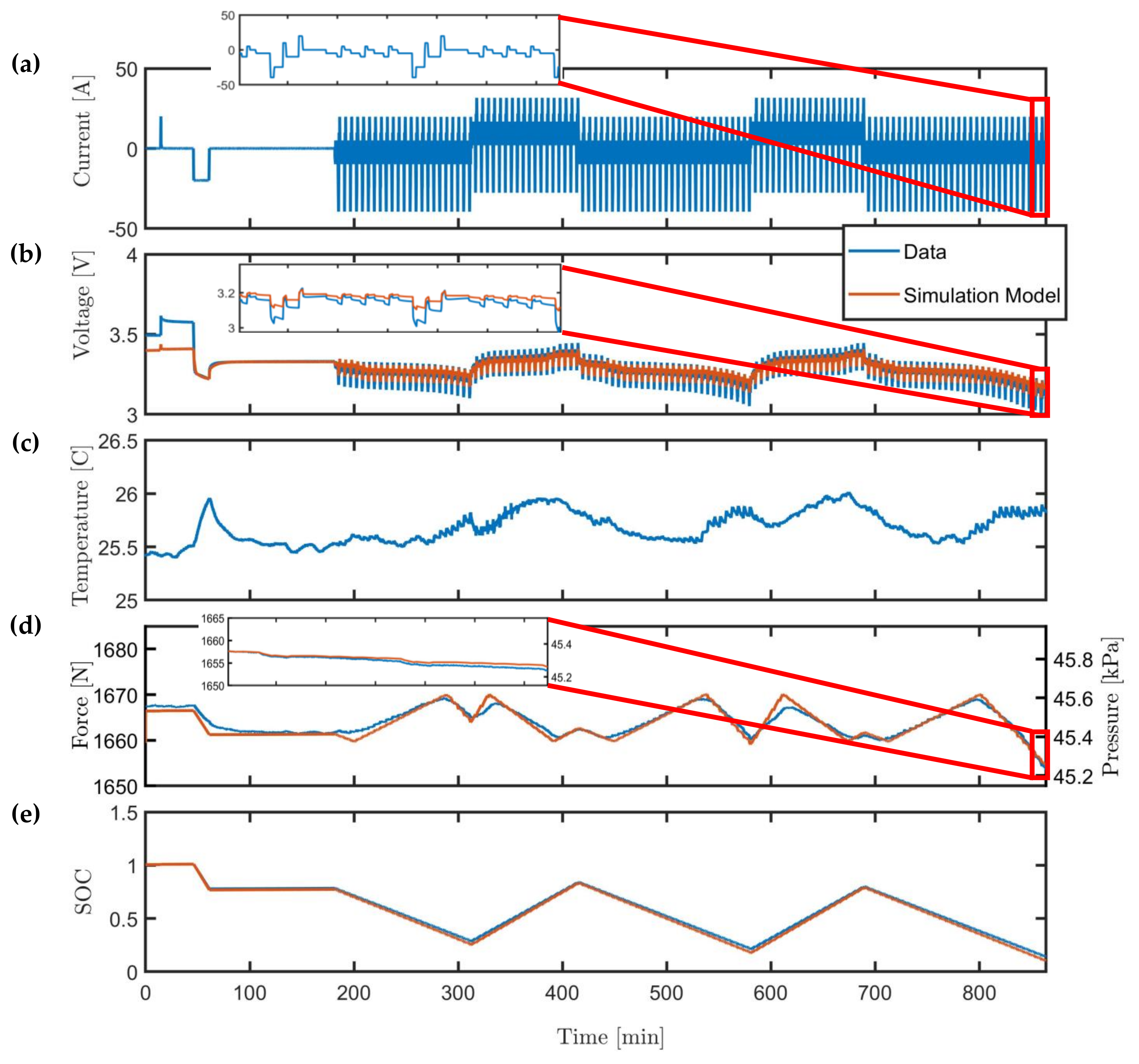
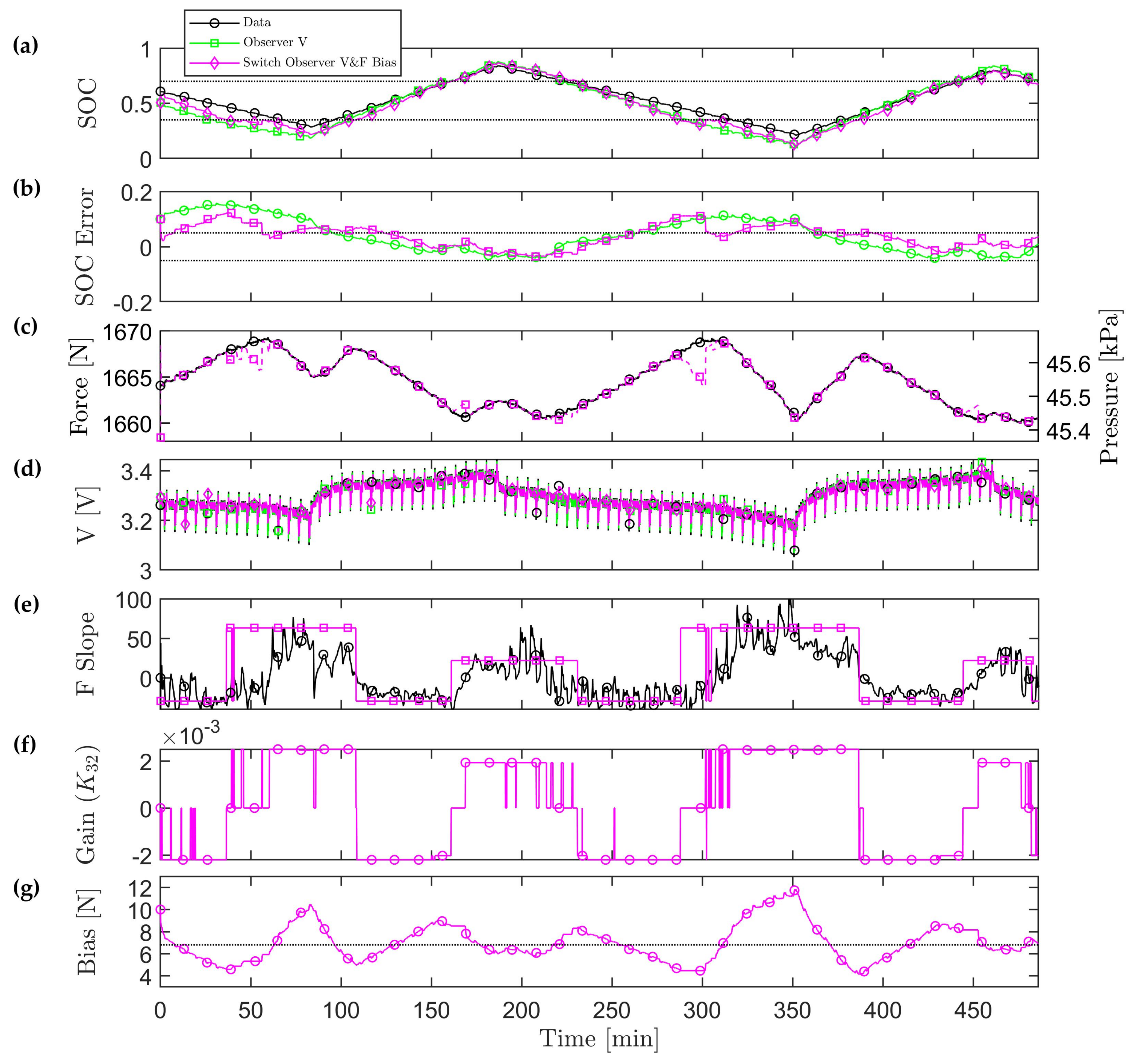
8. Experimental Data Results Using F–SOC and OCV–SOC

With a $10\%$ initial error in our SOC estimate, we obtain the results shown in Figure 8. The observer was initialized to 51% SOC, whereas the true state was 61% SOC, to highlight the performance in the middle SOC region where voltage based techniques are less effective. The current waveform discussed in Section 2 was applied to the battery and the observer. As in the simulated results, the proposed Switch Observer V&F Bias has faster convergence than the SOC estimation based on V alone as shown in Figure 8b. The V&F Bias observer exhibits lower RMSE, faster time convergence to the denoted SOC estimation error bound (EEB), and reduced maximum absolute SOC error, as shown in

Table 6. Comparison of the RMSE index for different initial estimate error and different sensors for data validation. V, terminal voltage; V&F Bias, fusion of both sensors.

Initial SOC Error	Parameters	Observer V	Switch Observer V&F
+10%	Time to 5% EEB [min]	95.5	0.18
	Max SOC Error [%]	11.89	11.79
	RMSE	0.0741	0.0611
−10%	Time to 5% EEB [min]	6.95	6.54
	Max SOC Error [%]	11.89	11.79
	RMSE	0.0594	0.0574

compared to V observer. The bias term oscillates around the estimated bias value of 6.8 N, as shown in Figure 8g. These larger oscillations in the bias could be due to our force data having additional dynamics besides the bias term. According to [13], the force has a dynamic term that is temperature dependent, and the ambient chamber temperature may oscillate within ±1 ${}^{\circ }$C. Therefore, this dynamic term should be added to our force model. There are some large errors in SOC estimation (approximately around 15%) at low SOC. This is due to our piecewise linear (PWL) fit.

In the area near 20% SOC, the PWL fit is less accurately, as shown in Figure 1, which results in increased SOC estimation error of around 10%. To better capture the non-linearity, the piecewise linear approximation could be further divided into more regions to provide a better fit. The weights chosen to obtain the gains $K_{1i}$ with $i=$ 1–4 and $K_{2i}$ with $i=$ 1–4 are shown in

Table 7. Control Weights for the different sensors for data validation: V,terminal voltage; V&F Bias, fusion of both sensors.

Models	Q	R
V	$diag(5,0.1,0.1)$	50
V&F Bias	diag(1,1×10${}^{-2}$,0.09,50)	$R=diag$(50,10,000)

. The gain $K_{32}$ that satisfies sign or is zero is shown in Figure 8f. The bias estimation state is initialized at 10 N.

9. Conclusions

In this paper, a new switching estimator design for a battery with the lithium ion LFP chemistry that integrates the non-monotonic F–SOC relation is proposed, verified by simulation, and validated using experimental data with respect to the SOC estimation accuracy. The estimator is based on switching PWL models that are scheduled according to the identified slope of the F–SOC operating point with a bias state in order to capture the drift exerted by the fixture and battery in our force measurement. Two different sensor scenarios, namely V and V&F Bias fusion, are compared, where it is concluded that the V&F Bias sensor improves the rate of SOC estimator convergence. This is due to the information added from the steeper, hence more informative, F–SOC characteristic than OCV–SOC relation despite large errors in the voltage and force models. The bounds on SOC estimation accuracy depend on the chosen inflection points of the F–SOC function. If they are correct, then the accuracy is better for the observer with both F and V than V only. Our future work will focus on determining if the drift on our force measurement is due to creep exerted by the poron and thermal expansion of the fixture or due to creep exerted by a degraded battery influenced by compressive stresses [32], or a combination of both. The thermal expansion term and swelling dynamic as a function of temperature will be considered. Data from an aged swelling cell will be used with the developed SOC estimator and the State of Health of the battery (SOH) will be estimated through the capacity fade. The inflection point model mismatch on the F–SOC function will be further studied in an aged cell since the inflection points change as the battery degrades or fades. Due to the tight manufacturing tolerances, the variability in thickness should not be a significant contributor to force measurement uncertainty. In terms of aging, the expected variability in the cell expansion is a subject of future studies. Cell-to-cell variability due to aging in the resulting force should also be investigated in future work based on initial findings from [14,15]. Finally, the measured force is the result of all cell’s expansion (summation) in a constrained module, therefore different levels of degradation for individual cells when charged in series would result in smoothing (convolution) of the force sensed on the module-level.

10. Disclaimer

Reference herein to any specific commercial company, product, process, or service by trade name, trademark, manufacturer, or otherwise, does not necessarily constitute or imply its endorsement, recommendation, or favoring by the United States Government or the Department of the Army (DA). The opinions of the authors expressed herein do not necessarily state or reflect those of the United States Government or the DA, and shall not be used for advertising or product endorsement purposes.

References

1. Cheng, K.W.E.; Divakar, B.P.; Wu, H.; Ding, K.; Fai, H. Battery-Management System (BMS) and SOC Development for Electrical Vehicles. IEEE Trans. Veh. Technol. 2011, 60, 76–88. [Google Scholar] [CrossRef]
2. Rahimi-Eichi, H.; Ojha, U.; Baronti, F.; Chow, M.Y. Battery Management System: An Overview of Its Application in the Smart Grid and Electric Vehicles. IEEE Ind. Electron. Mater. 2013, 7, 4–16. [Google Scholar] [CrossRef]
3. Chen, Z.; Fu, Y.; Mi, C. State of Charge Estimation of Lithium-Ion Batteries in Electric Drive Vehicles Using Extended Kalman Filtering. IEEE Trans. Veh. Technol. 2013, 62, 1020–1030. [Google Scholar] [CrossRef]
4. Zubi, G.; Dufo-López, R.; Carvalho, M.; Pasaogluc, G. The lithium-ion battery: State of the art and future perspectives. Renew. Sustain. Energy Rev. 2018, 89, 292–308. [Google Scholar] [CrossRef]
5. Satyavani, T.V.S.L.; Kumar, A.S.; Rao, P.S. Methods of synthesis and performance improvement of lithium iron phosphate for high rate Li-ion batteries: A review. Int. J. Eng. Sci. Technol. 2016, 19, 178–188. [Google Scholar] [CrossRef] [Green Version]
6. Malik, R.; Abdellahi, A.; Ceder, G. A critical review of the Li insertion mechanisms in LiFePO4 electrodes. J. Electrochem. Soc. 2013, 160, A3179. [Google Scholar] [CrossRef]
7. Xiong, R.; He, H.; Sun, F.; Zhao, K. Evaluation on State of Charge Estimation of Batteries With Adaptive Extended Kalman Filter by Experiment Approach. IEEE Trans. Veh. Technol. 2013, 62, 108–117. [Google Scholar] [CrossRef]
8. Zhang, C.; Wang, L.; Li, X.; Chen, W.; Yin, G.; Jiang, J. Robust and Adaptive Estimation of State of Charge for Lithium-Ion Batteries. IEEE Trans. Ind. Electron. 2015, 62, 4948–4957. [Google Scholar] [CrossRef]
9. Mohan, S.; Kim, Y.; Stefanopoulou, A. On Improving Battery State of Charge Estimation Using Bulk Force Measurements. In Proceedings of the ASME 2015 Dynamic Systems and Control Conference, Columbus, OH, USA, 28–30 October 2015. [Google Scholar]
10. Jones, E.M.C.; Silberstein, M.N.; White, S.R.; Sottos, N.R. In Situ Measurements of Strains in Composite Battery Electrodes during Electrochemical Cycling. Exp. Mech. 2014, 54, 971–985. [Google Scholar] [CrossRef]
11. Cannarella, J.; Leng, C.Z.; Arnold, C.B. On the Coupling between Stress and Voltage in Lithium-Ion Pouch Cells. In Proceedings of the SPIE Sensing Technology + Applications Energy Harvesting and Storage: Materials, Devices, and Applications, Baltimore, MD, USA, 5–9 May 2014. [Google Scholar]
12. Oh, K.; Siegel, J.; Secondo, L.; Kim, S.; Samad, N.; Qin, J.; Anderson, D.; Garikipati, K.; Knobloch, A.; Epureanu, B.; et al. Rate Dependence of Swelling in Lithium-Ion Cells. J. Power Sources 2014, 267, 197–202. [Google Scholar] [CrossRef]
13. Mohan, S.; Kim, Y.; Siegel, J.B.; Samad, N.A.; Stefanopoulou, A.G. A phenomenological model of bulk force in a li-ion battery pack and its application to state of charge estimation. J. Electrochem. Soc. 2014, 161, A2222–A2231. [Google Scholar] [CrossRef] [Green Version]
14. Samad, N.A.; Kim, Y.; Siegel, J.B.; Stefanopoulou, A.G. Battery capacity fading estimation using a force-based incremental capacity analysis. J. Electroche. Soc. 2016, 163, A1584–A1594. [Google Scholar] [CrossRef] [Green Version]
15. Mohtat, P.; Lee, S.; Siegel, J.B.; Stefanopoulou, A.G. Towards Better Estimability of Electrode-Specific State of Health: Decoding the Cell Expansion. J. Power Sources 2019, 427, 101–111. [Google Scholar] [CrossRef]
16. PORON® 4701-30 Polyurethane. Available online: https://rogerscorp.com/elastomeric-material-solutions/poron-industrial-polyurethanes/poron-4701-30 (accessed on 26 April 2020).
17. Kim, T.; Qiao, W.; Qu, L. A series-connected self-reconfigurable multicell battery capable of safe and effective charging/discharging and balancing operations. In Proceedings of the 2012 Twenty-Seventh Annual IEEE Applied Power Electronics Conference and Exposition (APEC), Orlando, FL, USA, 5–9 February 2012. [Google Scholar]
18. Shousha, C.M.; McRae, T.; Prodić, A.; Marten, V.; Milios, J. Design and Implementation of High Power Density Assisting Step-Up Converter With Integrated Battery Balancing Feature. IEEE Trans. Emerg. Sel. Top. Power Electron. 2017, 5, 1068–1077. [Google Scholar] [CrossRef]
19. Kim, Y.; Samad, N.A.; Oh, K.Y.; Siegel, J.B.; Epureanu, B.I.; Stefanopoulou, A.G. Estimating State-of-Charge Imbalance of Batteries Using Force Measurements. In Proceedings of the 2016 American Control Conference (ACC), Boston, MA, USA, 6–8 July 2016. [Google Scholar]
20. Huang, W.; Qahouq, J.A.A. Energy sharing control scheme for state-of-charge balancing of distributed battery energy storage system. IEEE Trans. Ind. Electron. 2015, 62, 2764–2776. [Google Scholar] [CrossRef]
21. Knobloch, A.; Kapusta, C.; Karp, J.; Plotnikov, Y.; Siegel, J.B.; Stefanopoulou, A.G. Fabrication of Multimeasurand Sensor for Monitoring of a Li-Ion Battery. J. Electron. Packag. 2018, 140, 031002. [Google Scholar] [CrossRef]
22. Polóni, T.; Figueroa-Santos, M.; Siegel, J.; Stefanopoulou, A. Integration of Non-Monotonic Cell Swelling Characteristic for State-of-Charge Estimation. In Proceedings of the 2018 Annual American Control Conference (ACC), Milwaukee, WI, USA, 27–29 June 2018. [Google Scholar]
23. Lee, S.; Mohtat, P.; Siegel, J.; Stefanopoulou, A. Beyond Estimating Battery State of Health: Identifiability of Individual Electrode Capacity and Utilization. In Proceedings of the 2018 Annual American Control Conference (ACC), Milwaukee, WI, USA, 27–29 June 2018. [Google Scholar]
24. Usabc Electric Vehicle Battery Test Procedures Manual, Appendix j-Detailed Procedure. Available online: https://www.uscar.org/guest/article_view.php?articles_id=74 (accessed on 26 April 2020).
25. Domenico, D.D.; Stefanopoulou, A.; Fiengo, G. Lithium-Ion Battery State of Charge and Critical Surface Charge Estimation Using an Electrochemical Model-Based Extended Kalman Filter. J. Dyn. Syst.-Trans. ASME 2010, 132, 061302. [Google Scholar] [CrossRef]
26. Forman, J.C.; Moura, S.J.; Stein, J.L.; Fathy, H.K. Genetic parameter identification of the Doyle-Fuller- Newman model from experimental cycling of a LiFePO4 battery. In Proceedings of the 2011 American Control Conference, San Francisco, CA, USA, 29 June–1 July 2011. [Google Scholar]
27. Pletcher, D. Electrochemistry: Volume 8; Royal Society of Chemistry: London, UK, 2007. [Google Scholar]
28. Hu, X.; Li, S.; Peng, H. A Comparative Study of Equivalent Circuit Models for Li-Ion Batteries. J. Power Sources 2012, 198, 359–367. [Google Scholar] [CrossRef]
29. Perez, H.E.; Siegel, J.B.; Lin, X.; Stefanopoulou, A.G.; Ding, Y.; Castanier, M.P. Parameterization and Validation of an Integrated Electro-Thermal Cylindrical LFP Battery Model. In Proceedings of the ASME 2012 5th Annual Dynamic Systems and Control Conference Joint with the JSME 2012 11th Motion and Vibration Conference, Fort Lauderdale, FL, USA, 17–19 October 2012. [Google Scholar]
30. Plett, G.L. Battery Management Systems, Volume I: Battery Modeling; Artech House: Boston, MA, USA, 2015. [Google Scholar]
31. Lewis, F.L. Optimal Estimation: With an Introduction to Stochastic Control Theory; Wiley: New York, NY, USA, 1986. [Google Scholar]
32. Peabody, C.; Arnold, C.B. The Role of Mechanically Induced Separator Creep in Lithium-Ion Battery Capacity Fade. J. Power Sources 2011, 196, 8147–8153. [Google Scholar] [CrossRef]
Figure 1. Measured voltage and force for the 20 Ah A123 lithium ion iron phosphate battery cycled under low current rate C / 20 . (a) Measured discharge (blue), charge (red), and average of discharge and charge (black) voltage for a C / 20 cycle. For military robots such as the Packbot shown above, SOC estimation is critical to avoid the robot getting stranded. Lithium ion iron phosphate (LFP) batteries are typically used for operation of this robot due to the high power required. (b) Measured discharge (blue), charge (red), and average of discharge and charge (black) force for the under current rate C / 20 . The experimental battery fixture consists of: (1) load cell (force sensor); (2) movable plate; (3) lithium ion battery; (4) two aluminum end-plates; (5) temperature sensor. For generalization of the results to the other cell sizes, the force measurements can be converted to pressure by diving the force by the surface area of our battery ( A b ), which is the width ( w b = 0.161 m) times the length ( l b = 0.227 m) of the battery, A b = w b × l b m 2 .
Energies 13 02653 g001
Figure 2. Drift in the force sensor can be observed by comparing the force vs. SOC for two C 20 cycles which were conducted two months apart with three cycles done in between them with the same battery. The force measurements have a minimum of 3 N and a maximum of 6 N drift across the entire SOC range. The drift could be caused by thermal expansion of the battery, pad, and fixture [13], capacity change, or a combination of all four throughout the life of the cell and module on which measurements are performed. Adjustments in the fixture and changes in the preload will cause larger changes in measured force but can also be modeled as a sensor drift. For generalization of the results to the other cell sizes, the pressure is shown.
Energies 13 02653 g002
Figure 3. A piecewise linear approximation of the (a) open circuit voltage and (b) cell swelling force was fit to the experimental measured values for the A123 Lithium Iron Phosphate Battery Cell. The gray dots correspond to the average of measured data at each SOC point from the charge and discharge cycles at the C 20 rate (see Figure 1). The orange line represents the PWL fit. The horizontal solid lines represent the inflection points of the cell swelling force. The horizontal dashed black lines represent the inflection points of the cell swelling force used for the developed observers. R I , R I I , and R I I I represent the force slope regions determined by our PWL model. For the PWL force model, we assume b L = c 3 and b H = c 5 since the changes in voltage and force slopes are due to the intrinsic phase transitions in the material of the battery electrodes [15]. Assessment of the SOC estimator robustness is performed by imposing b ^ L b L and b ^ H b H to capture model mismatch for the force and voltage behavior. For generalization of the results to the other cell sizes, the pressure is shown.
Energies 13 02653 g003
Figure 4. Comparison of open loop simulation model results (denoted by the color orange) and experimental measurement of voltage, temperature, force, and SOC obtained from the 20 Ah battery during the Dynamic Stress Test (DST) inside an environmentally controlled chamber set at 25 C ambient conditions. (a) Current profile scaled for the 20 Ah A123 battery. (b) Comparison of the open loop model terminal voltage and measurement. (c) Measured battery temperature. (d) Comparison of the open loop modeled force and measured force. After 30 min of rest, the un-modeled dynamics in force excited by cycling of the cell to decay to zero. For generalization of the results to the other cell sizes, the pressure is shown. (e) Comparison of state of charge (SOC) measurement.
Energies 13 02653 g004
Figure 5. Simulation (without bias in the force measurement) for the Switch Observer V&F developed in our previous work [22]. This figure shows the impact of high gains corresponding to solution of the linear quadratic estimator using Q 1 = diag ( [ 2 , 0.1 , 0.1 ] ) and R = diag ( [ 1 , 1 ] ) with moving windows of length (MW) = 150 and MW = 450. If the gain is lowered by using Q 2 = diag ( [ 2 , 0.1 , 1 e 2 ] ) , as shown by the purple dashed line, the error is decreased by 5% with same 150pt moving window length. (a) Comparison of the simulated state of charge (SOC). (b) Comparison of the state of charge (SOC) error with the dashed lines representing the target ±5% bound. (c) Comparison of the simulated force. For generalization of the results to the other cell sizes, the pressure is shown. (d) Comparison of the true slope with the estimated slope d F ˜ d z and observer output. Due to the greater delay ( δ ) before applying the zero gain for the MW = 450 case, a higher error in SOC estimation occurs during the transition from R I I to R I . (e) Comparison of the feedback gain K 32 from force to SOC based on the switching logic. When the observer and estimated slopes mismatch, the gain is set to zero.
Energies 13 02653 g005
Figure 6. Simulation assuming accurate modeling using Switch Observer V&F Bias observer with an emulated bias of 3 N and 10 % (0.1) initial SOC error. (a) Comparison of the simulated state of charge (SOC). Is clear from the results that Switch Observer V&F without bias estimation diverges from the simulated SOC. Therefore, bias estimation is needed in the developed observer. (b) Comparison of the state of charge (SOC) error with the dashed lines representing the target ±5% bound. SOC errors greater than 20% are obtained with the Switch Observer V&F without bias estimation. It is shown that with bias estimation the SOC error is within the 5% estimation error bound (EEB). (c) Comparison of the simulated force and observer outputs. The bias state permits deviation in the force output, without compromising SOC estimation. For generalization of the results to the other cell sizes, the pressure is shown. (d) Comparison of the simulated terminal voltage. (e) Comparison of the true slope with the estimated slope d F ˜ d z and observer output. (f) Comparison of the feedback gain K 32 from force to SOC based on the switching logic. As shown in region A, denoted by the black dashed horizontal lines, when the observer and estimated slopes mismatch, the gain is set to zero. (g) The observer estimates the bias state which converges to the true bias as shown by the black horizontal dashed lines.
Energies 13 02653 g006
Figure 7. Simulation of the impact of model mismatch in the inflection points of the force vs. SOC curve. A 10% error in b ^ L and b ^ H is tested for the observer (Switch Observer V&F Bias) with an emulated bias of 3 N and 10% (0.1) initial SOC error. (a) Comparison of the simulated state of charge (SOC). (b) Comparison of the state of charge (SOC) error with the dashed lines representing the target ± 5 % bound. The SOC error converges to within the ± 5 % error bound. The largest SOC errors are observed near the switching points denoted by the horizontal dashed lines in Figure 7a. (c) Comparison of the simulated force and observer output. For generalization of the results to the other cell sizes, the pressure is shown. (d) Comparison of the simulated terminal voltage and observer output. (e) Comparison of the true slope with the estimated slope d F ˜ d z and observer output. (f) Comparison of the feedback gain K 32 from force to SOC based on the switching logic. The gain is set to zero when there is mismatch in the estimated slope and that based on the observer SOC. (g) The Bias state estimate converges slowly. The impact of model mismatch in the inflection points of the force vs. SOC curve can be seen by comparing the (Switch Observer V&F Bias Mismatch) and (Switch Observer V&F Bias) which uses the correct value. The accurate observer converges to the true value of 3 N, denoted by the dashed horizontal line whereas mismatch leads to a constant over-estimate of about 1 N.
Energies 13 02653 g007
Figure 8. Experimental validation of the developed observer (Switch Observer V&F Bias) with 10% (0.1) initial SOC error. The offline experimentally measured current, voltage, and force data were fed into the model to assess performance. (a) Comparison of high accuracy coulomb counting based state of charge (SOC) with observer estimates. (b) Comparison of the state of charge (SOC) error with the dashed lines representing the target ± 5 % bound. The observer with force bias state estimation demonstrates better performance. The large error at low SOC for both observers is due to model mismatch the piecewise linear OCV–SOC fit at low SOC. (c) Comparison of measured and estimated force. (d) Comparison of the experimental and observer modeled terminal voltage. (e) Comparison of the estimated slope d F ˜ d z and observer model. (f) Comparison of the feedback gain K 32 from force to SOC based on the switching logic. (g) The Bias state estimate fluctuates around the average value (denoted by the horizontal dashed line). This could be due model mismatch, where the force error is exciting the bias state estimate.
Energies 13 02653 g008