Abstract
Greenhouse gas emission is one of the main environmental issues of today, and energy savings in all industries contribute to reducing energy demand, implying, in turn, less carbon emissions into the atmosphere. In this framework, water pumping systems are one of the most energy-consuming activities. The optimal regulation of pumping systems with the use of variable speed drives is gaining the attention of designers and managing authorities. However, optimal management and operation of pumping systems is often performed, employing variable speed drives without considering if the energy savings are enough to justify their purchasing and installation costs. In this paper, the authors compare two optimal pump scheduling techniques, optimal regulation of constant speed pumps by an optimal ON/OFF sequence and optimal regulation with a variable speed pump. Much of the attention is devoted to the analysis of the costs involved in a hypothetical managing authority for the water distribution system in order to determine whether the savings in operating costs is enough to justify the employment of variable speed drives.
1. Introduction
Energy consumption in Water Distribution Networks (WDNs) and Water Supply Systems (WSS) is typically one of the greatest marginal costs, as they constitute a significant portion of the energy demand. WSSs and WDNs are systems designed to transport water over large areas to the population and they have a significant environmental impact. Indeed, a huge amount of energy consumption and related greenhouse gas emissions are due to pumping systems, and water losses are involved. In the entire water sector, the energy consumption associated to pumping systems represents the largest portion [1], which, in some cases, amounts to 90% [2].
Smart management strategies for pumping stations (e.g., optimal pump regulation) are increasingly attracting the interest of researchers. Moreover, the energy consumed by pumping systems has an environmental impact as well, because it is part of the energy demand and then contributes to the increase in greenhouse gas emissions. Optimal pump scheduling (OPS) can be performed in two ways: with the classical ON/OFF regulation of pumps working at constant speed of by either ON/OFF and pump speed regulation.
In the literature, many efforts have been dedicated to the OPS problem, but the main focus has been on the best kind of optimization model. A linear programing model was employed in [3] to seek the minimum energy consumption by the classic ON/OFF regulation of pumps. A non-linear programming algorithm for the determination of the optimal scheduling of hydro-pumped systems was considered in [4]. Many authors resorted to heuristic approaches to minimize the energy consumption in WDNs or WSSs due to their flexibility and ease of use. A simulated annealing algorithm was used in [5] to determine the optimal operation of water systems (including pumps). An ant colony optimization method was employed in [6] to minimize the energy consumption of pumping systems by determining the optimal ON/OFF time intervals of the pumps. A genetic algorithm was used by [7] to derive the optimal operational rules in WDNs. In [8] a particle swarm optimization algorithm was used to minimize the energy consumption of pumping stations in WDNs. To improve the performance of a heuristic algorithm, hybrid methods were also employed in the minimization of the energy consumption of pumps in WSSs [9].
In all the aforementioned papers, pumps are modelled as constant speed pumps (CSPs), and then an optimal control rule is used to attain the minimum energy consumption is based on the classical ON/OFF pump sequence.
When pumps are modelled as Variable Speed Pumps (VSP), the control rule is based on a rotational speed at which the pumps must operate at a given time, and this is accomplished employing variable speed drives (VSDs). In general, the use of VSDs may lead to over 10% of energy savings with respect to CSPs [10]; however, fewer works have been dedicated to optimal pump regulation through VSDs. A decision support system tool for optimal WDNs operations, including pumping systems, was proposed in [11], while a comparison of different optimization methods for the optimal scheduling of pumps in WDNs with both CSPs and VSPs was presented in [12]. For a more comprehensive review of optimal WDN operations, interested readers may refer to the literature review by [13].
By reducing the energy consumption, VSDs help to reduce the maintenance costs as well. As a matter of fact, a reduction in energy consumption and an improvement in pump performance may lead to a reduction in maintenance and repair costs. Indeed, these costs range from 30% to 70% of the annual energy costs [14], while, according to [15] the energy, purchase/installation and repair/maintenance costs amount to 64%, 9% and 27%, respectively. Therefore, any reduction in the energy consumption and improvement to the pump performance directly results in savings in the aforementioned costs.
In most of the literature related to the optimal regulation of VSPs, the authors still focused on the optimization method adopted and concluded that the energy savings obtained with VSPs was higher than CSPs. However, none of the authors demonstrated if the reduction in energy costs was enough to justify the employment of VSDs, as the purchase and installation such devices entails additional costs. From the data collected by [16], the installation cost of a VSD may vary from 3000 USD for a 5 horsepower (HP) pump, to 45,000 for a 250 HP pump, with a cost per HP that ranges from 600 USD to 200 USD per HP. Consequently, the VSD purchasing cost cannot be justified by the energy savings if the payback period exceeds the lifetime cycle of the pumping system. This latter aspect has not been investigated within the scientific literature on optimal pump operation in WDNs.
In this paper, the results obtained in terms of energy savings by the optimal regulation with VSPs versus CSPs (ON/OFF regulation) are analyzed, and optimizations are carried out by means of a specific Genetic Algorithm (GA) in both cases. The optimal regulation of both CSPs and VSPs is applied to two WDNs from the literature, and the solutions are compared in terms of energy savings and an economic analysis of the solutions is carried out to demonstrate if the use of VSDs is always justified by the increase in energy savings. This last aspect has not been contemplated within the related literature.
2. Problem Description
2.1. Methodology
In this work, the optimal regulation of pumping systems in WDNs is performed with both CSPs and VSPs. The results obtained are compared from an economic point of view to establish whether the additional costs to purchase VSDs is justified. The procedure employed within this manuscript is reported in Figure 1.
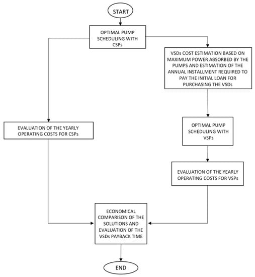
Figure 1.
Flow chart of the proposed procedure.
The optimal scheduling of CSPs is first performed; based on the maximum absorbed power of the pumps, the VSD cost is estimated. The optimal regulation of pumping systems is then performed, considering VSPs. Finally, the costs of the optimal solution with CSPs and VSPs are compared in order to establish if the savings in energy costs obtained with VSPs are enough to justify the additional costs of the purchase and installation of VSDs.
2.2. Working Hypothesis
The procedure described in the previous section is applied to two WDNs taken from the scientific literature. The hypothesis that the WDNs already exist is made, and then the goal of the optimizations is to minimize the total operational cost of the pumping systems. The two cases of study are not real WDNs, although they are realistic, and the pumps used to feed the networks are not commercial. For this reason, it is hard to estimate the maintenance and repair costs of the pumps and of the VSDs as well. Herein, the authors resorted to the literature to estimate the costs for the purchase and installation of the VSDs: the pumps’ maximum absorbed power is first evaluated from the CSP optimization, then the VSD costs are estimated by considering a unitary per horsepower (HP). In addition, the costs for the maintenance and repair of the pumps are assumed to be proportional to the yearly energy cost, as also suggested by the literature. Therefore, the minimization of the energy consumption is equivalent to minimizing all of the operating costs.
2.3. Optimization Problem Formulation
The Optimal Pump Scheduling (OPS) problem consists of seeking a sequence of hourly relative pump speeds, such that minimum energy consumption is achieved during an operating cycle. The relative speed V is defined as the ratio between the pump rotational speed (rpm) and the pump characteristic rotational speed (rpm). In the case of the ON/OFF sequence, the relative speed during the i-th time interval of the day of the j-th pump , meaning that only one (OFF) or zero (ON) can be assumed by the decision variable; when VSD are employed, , where Vmin is the minimum relative speed at which the pump can operate. The feasibility of the solutions is ensured by the hydraulic constraints—that is, adequate network pressure levels, adequate water tank levels and the recovery of water volumes supplied by the tanks at the end of the scheduling horizon. In addition, technical constraints related to the pump operations must be also considered in order to reduce pump maintenance.
The problem can be formulated as follows:
subject to
where: is the number of time intervals into which the scheduling horizon is divided; is the number of pumps; Ce is the total energy cost; γ is the specific weight of water; and are the flow and head, respectively, of the j-th pump during the i-th time interval; is the efficiency (defined as the product of hydraulic, mechanical and volumetric efficiency), of the j-th pump during the i-th time interval; Ci is the energy tariff during the i-th time interval; is the water level within the r-th tank during the i-th time interval; , and are, respectively, the minimum, maximum and initial water level within the tank; and are the number of actuation of the j-th pump and the maximum number of actuation allowed for the j-th pump, respectively.
Equation (1) represents the minimization of the total energy cost expressed as the sum of the energy absorbed by each pump at every operational time interval times its energy tariff. Equations (2) and (3) are the constraints related to the water level within the tanks. It must range between a maximum and a minimum level, to avoid spilling water from the overflow and the tank emptying, respectively. In addition, the water level within the tanks at the end of the scheduling horizon must be at least equal to that at the beginning in order to guarantee that water volume within the tanks does not lessen during the day. Equation (4) is a constraint used to maintain adequate pressure levels within the network. Equation (5) is used to bound the number of pump actuations within the operational cycle, forcing them to be less or equal to a pre-assigned number. This will influence the maintenance cost of the pumps, since the more they are switched on during the scheduling period, the greater the wear will be [17]. Finally, Equation (6) represents a constraint introduced to assure that the maximum discharge lifted by the j-th pump does not exceed the pump operating range (i.e., the maximum discharge according to the pump characteristic curves).
2.4. The Proposed Genetic Algorithm
The proposed GA was implemented in the VB.NET™ environment. It is the same algorithm used by the first author in other works (see [18,19] for more details). The difference between the case of CSP and VSP is only in the decision variable representation: when CSP are considered (ON/OFF only), the decision variables (Vi,j) can assume values that are equal only to zero or one. Therefore, the chromosome is represented by a sequence of 1 bit binary variables of length equal to the number of pumps multiplied by the number of intervals in which the day has been divided (typically 24 h). In the case of VSP, a sequence of 5 bit decision variables is considered to represent the possible values of relative speeds, implying that the chromosome has a length equal to the number of VSPs multiplied by the number of intervals. In particular, each decision variable can assume the value zero plus 25-2, in which the interval [Vmin, 1] is discretized.
Genetic algorithms are designed for unconstrained optimization and, in order to handle constraints, the penalty function method is usually employed. Herein, the same penalty functions described in [18] are used for constraints handling to penalizing solutions that violate Equations (2)–(6).
Finally, the GA was implemented using multipoint crossover (with three cutting points), exponential ranking selection (with parameter equal to 0.05), mutation (with mutation probability equal to 0.01) and the elitist operator (with just one individual preserved from each generation). Equally, the maximum number of generations (equal to 500), was used as stopping criterion, and the number of individuals (candidate solutions) was equal to 100 for each generation.
2.5. Hydraulic Modelling of VSP
The hydraulic solver is based on EPANET2.0™ [20], and it is linked within our program through the dynamic link library (DLL). Given the energy price pattern, daily demand patterns, pump head/flow curves and pump efficiency curves, EPANET2.0™ provides the daily energy cost of each solution as well as the hydraulic conditions (pressure at nodes, links flow, water tank levels, etc.).
In order to model variable speed pump, the EPANET2.0™ software already employs the classical affinity laws, which are:
where , and are, respectively, the j-th pump head, flow and absorbed power during the i-th time interval; while , and are, respectively, the j-th pump head, flow and absorbed power when the pump is running at its characteristic speed (i.e., ).
The only issue is relative to Equation (9), because that affinity law is valid only when the setting speed does not differ more than 15–20% from the characteristic speed. However, as will be specified in the presentation of the two cases of study, the minimum relative speed will not exceed this difference, and then Equation (9) can be adopted herein.
2.6. The Estimation of the Costs
The two cases of study considered herein are taken from the literature, but costs related to the maintenance and repair of the pumping stations are not provided. Furthermore, the costs of purchase and installation of VSDs are required to perform an economic analysis of the solutions. With this aim, the authors resorted to the literature to retrieve the aforementioned costs. By a worldwide investigation of the costs related to the life cycle of a pumping system performed by [15], the energy cost represents 64% of the total, while maintenance and repair costs amount to 27%. Furthermore, to estimate the costs related to purchasing and installing VSDs, the authors referred to the work of [16]. In particular, the VSD costs ranged from 600 USD per horsepower (HP) for small pumps, (e.g., 5 HP), to about 200 USD per HP for pumps up to 250 hp. However, for powers ranging from 30 HP to 250 HP the cost per HP does not vary too much, and can be considered approximately constant and equal to 200 USD/HP. With that being said, in this work, we hypothesize that the costs for maintenance and repair are proportional to the energy cost. This is also consistent with the fact that the more the pump absorbs power, the more it wears (increased heating, increased component wear, etc.), and this is particularly true when the pump works far from its best efficiency point (BEP) (more energy consumption and more pump wear). Therefore, if the energy costs (Ce) represent 64% of the total Life Cycle Costs (LCC), and maintenance and repair costs are 27%, it can be demonstrated that Cmr is about 42.2% of Ce, and this value is consistent with data from the literature [14], according to which maintenance and repair costs range from 30% to 70% of the cost of the energy. To estimate the VSD costs, a constant value of 200 USD/HP is considered, and HP are computed from the power absorbed by the pumps with the ON/OFF regulation, which will be considered the reference condition.
The estimation of the payback period is performed by computing the amortization rate Ar by the well-known formula
where n is the payment period and i is the interest rate. The values n = 10 and i = 0.05 are considered herein, corresponding to . Then, when the VSDs are employed, the difference between the solution with CSP and VSP will be used to justify the purchase and installation cost of the VSDs, to establish if VSDs are convenient. In the latter case, the costs over the years are evaluated as:
where is the cost during the y-th year, are the costs for purchasing and installing VSDs and
are the operating costs.
Because Cy is a function of the energy costs, the minimization of Equation (1) is equivalent to the minimization of the yearly costs.
2.7. Cases of Study
To carry out our analyses, two WDNs were chosen from the literature. These WDNs were chosen because they were the subject of several works dealing with optimal pump scheduling with ON/OFF regulation and they can serve as the starting hypothesis for our work. The first case of study is a WDN, first proposed by [8], while the second and more complex WDN is called Anytown Modified [20]. For these two cases of study, it is assumed that the pumping station plant already exists, and the optimal solutions with CSPs expressed as sequence of optimal ON/OFF are the reference conditions. In particular, the minimum relative speed Vmin at which the pumps can run is 0.8 rpm/rpm for Case 1 and 0.9 rpm/rpm for Case 2. Below this relative speed, the existing pumps cannot deliver sufficient head.
2.7.1. Case 1—Van Zyl et al. (2004) WDN
The first WDN (Case 1) was proposed by [21], and its layout is reported in Figure 2.
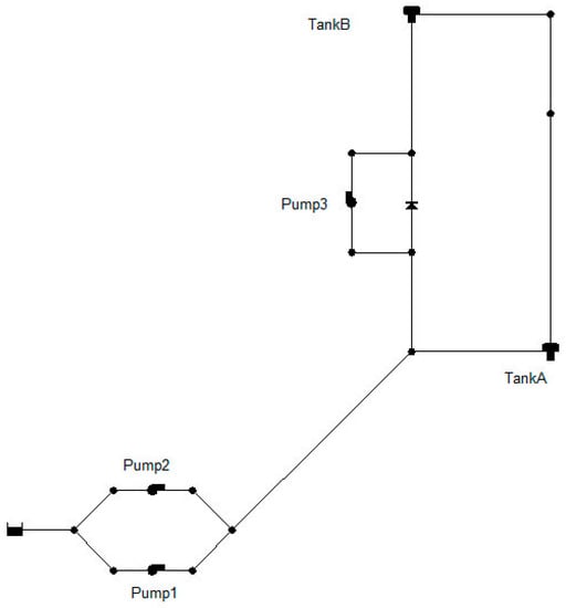
Figure 2.
Case 1—Van Zyl et al. (2004), Water Distribution Network (WDN).
This network is fed by two pumps (Pump 1 and Pump 2), plus one pump acting as a booster (Pump 3), one reservoir, two tanks, 15 pipes and 13 nodes, two of which are demand nodes. The users demand that the two demand nodes follow a daily pattern that is reported in the paper by [21] with all the data concerning the network characteristics (pipe diameter, node elevation, pump characteristic curves, etc.). Interested readers may refer to the cited paper to retrieve all network data, which are not reported herein for the sake of brevity. For Case 1, pump efficiency curves were provided only for Pump 1 and Pump 2, and then VSD were considered only for these two pumps, while Pump 3 works at constant speed. Despite the fact that Case 1 was considered in several papers from the literature [6,21,22], the authors performed an optimization to determine the best solution with ON/OFF regulation, obtaining the best result so far (see Table 1) for this network. The pumps’ ON/OFF patterns are reported in Figure 3 (the histogram when each pump is active).

Table 1.
Comparison of the best literature solutions for Case 1 with ON/OFF regulation.
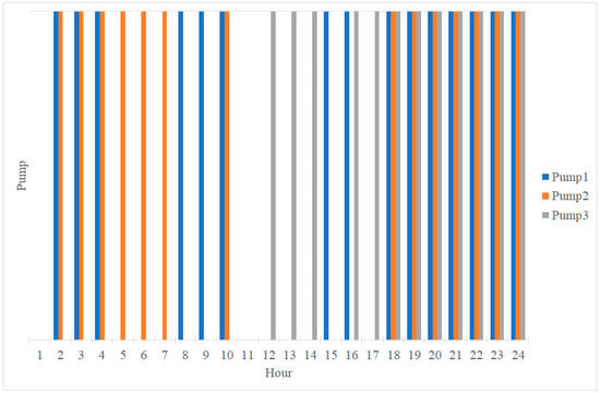
Figure 3.
Best ON/OFF patterns solution.
The results obtained herein with ON/OFF regulation will be used as a reference condition to estimate the costs. The yearly cost for energy purchase is 165,741.85 USD/year, and from the consideration given in Section 2.5, the costs for the maintenance and repair of pumps amount to 69,943.06 USD/year. Therefore, the yearly operating costs are Cop = 235,684.91 USD/year which is considered a constant cost. Following the results of the numerical simulations, it was possible to evaluate the peak power absorbed by the pumps, and then estimate the costs for the VSD, considering a cost of 200 USD per Horsepower (HP), as reported in Table 2.
Table 2.
Variable speed drive (VSD) cost estimation for Case 1.
Therefore, the purchasing of VSDs for Pump 1 and Pump 2 entails an additional cost of 112,032.68 USD for two VSDs.
2.7.2. Case 2—Anytown Modified (ATM) Network
The network was proposed in [23] and it is comprised of 41 pipes, 19 nodes, three storage tanks, a supply source, and three identical pumps in parallel. A schematic of the network is reported in Figure 3.
All data about this network and the problem constraints can be found in [19]. In this case, the best solution obtained in the literature, with CSPs costing 3575.5 USD/day, and the optimal ON/OFF sequence is reported in Figure 4 (again, the histogram when each pump is active).
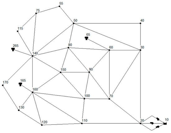
Figure 4.
Case 2—Anytown Modified Network.
Because the pumps are all of the same type, three identical VSDs can be used. From the results obtained by the simulation, it was possible to quantify the maximum energy absorbed, and then estimate the VSD price (Table 3).
Table 3.
VSD cost estimation for Case 2.
Therefore, the total costs for purchasing and installing three VSDs amount to 410,031.50 USD, the yearly energy cost is Ce = 1,305,057.50 USD/year, and the yearly maintenance and repair costs are Cmr = 550,734.27 USD/year, for a total yearly operating cost of Cop = 1,855,791.77 USD/year. The yearly costs are quite high in this case, but the use of VSDs may lower both Ce and Cmr enough to save money.
3. Application and Discussion of Results
In this section, the optimal regulation of pumps is performed by optimizing the sequence of hourly relative pump speeds. The results obtained are discussed in terms of both behavior and economical solutions.
3.1. Application to Case 1
The optimization algorithm is applied to Case 1 to seek the minimum energy consumption during the day. To account for the GA parameter uncertainties, ten optimizations are performed by varying the initial seed from one to 10. The best solution obtained was a 290.36 USD daily energy cost, and the sequence of pump relative speeds is reported in Figure 5.
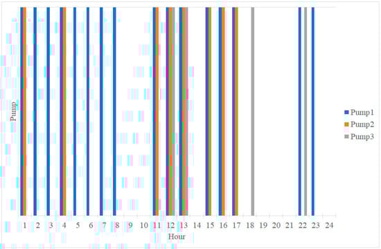
Figure 5.
Optimal ON/OFF sequence of Anytown Modified (ATM) network (Cimorelli et al., 2020).
Upon inspection of Figure 6, it is evident that the number of pump switches were fewer those in the case of CSP. Pump 1 was switched on three times, Pump 2 was switched on once and Pump 3 was also switched on only once, but because they were working at lower relative speeds, they were able to absorb less power. Even though the minimum relative speed Vmin = 0.8 rpm/rpm in this case, according to Equation (9), the power drops down to about 50%, implying huge energy savings [24]. Furthermore, the average efficiency of the pumps is higher in the case of VSDs: with the constant speed pump, the average efficiencies are 75.17%, 76.77% and 85% for Pumps 1, 2 and 3, respectively, while, with VSDs, the average efficiencies are 77.99%, 77.96% and 85% for Pumps 1, 2 and 3, respectively. The annual installment for the purchase and installation of the two VSDs is 14508.75 USD, thus leading to a yearly total cost of Cy = 165,214.30 USD, with a difference of only 575.55 USD with respect to the solution with CSPs. This small difference is due to the fact that, with VSPs, the purchase and installation costs for two VSDs must be considered with an amortization rate given by Equation (11). In Figure 7, the cumulative total and operating costs are reported (left and right panel, respectively).
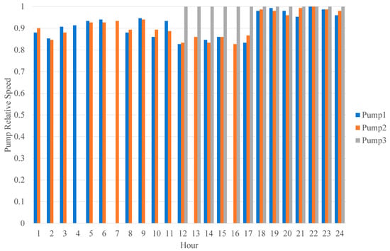
Figure 6.
Hourly sequence of pumps relative speeds for Case 1.
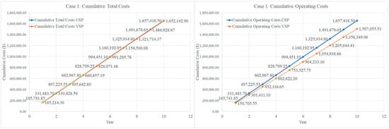
Figure 7.
Case 1: Cumulative total (left) and operating (right) costs with both constant speed pumps (CSPs) and VSPs.
After a period of 10 years, the difference between the cumulative costs is only 5275.53 USD, although the difference between the operating costs (energy, maintenance and repair) is quite large (150,362.99 USD after 10 years). However, to repay the initial loan for the purchase and installation of two VSDs, an amount of 145,087.46 USD is required over the 10-year period. Therefore, the payback time for the two VSDs is 10 years, meaning that the actual money saving occurs from the 10th year onwards, which is a quite long period to wait, leading us to the conclusion that, in this case, VSDs are not particularly convenient, because after 10 years the costs for the maintenance of VSDs usually tends to increase because such period would be close to their life expectancy (10 years on average).
3.2. Application to Case 2
The application of the optimization algorithm to Case 2 was performed by the program 10 times with initial seeds varying from one to 10. The best solution obtained with VSPs is characterized by a daily cost for energy Ce = 3341.60 USD/Day, and it is a noticeable difference given that Vmin = 0.9 rpm/rpm for Case 2. However, according to Equation (9), when a pump is running at 0.9 rpm/rpm of relative speed, the absorbed power drops down to 73%, thus allowing enough of an energy saving. The optimal sequence of relative speeds for the three pumps is reported in Figure 8.
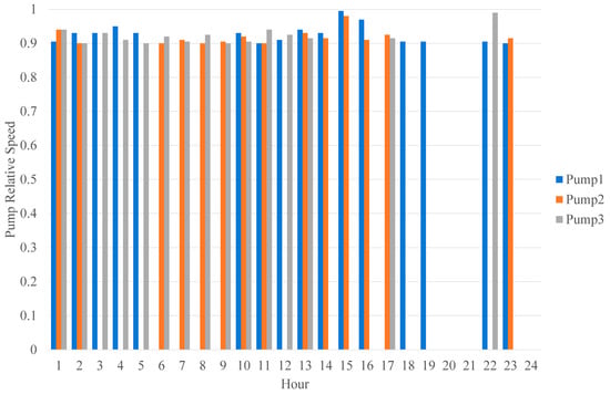
Figure 8.
Optimal sequence of relative pump speeds for Case 2.
In contrast to the previous case, the pumps were switched on more frequently: Pump 1 and 2 were switched on three times and Pump 3 was switched on twice (the maximum number of switches in this case is three per day; see [19]) and, as can be seen from Figure 7, most of the time, the pumps are working close to the minimum relative speed.
In addition, the efficiencies of the pumps when VSDs are employed are higher than constant speed pumps. Indeed, with constant speed pumps, the average efficiency is 58.39%, 56.38% and 58.48% for Pumps 1, 2 and 3, respectively, while, when VSDs are used, the average efficiencies are 60.40%, 58.07% and 58.54% for Pumps 1, 2 and 3, respectively.
In the case of VSPs, the yearly operating costs (Equation (12)) amount to 1,734,390.65 USD/year, while the annual installment required to pay the loan for the initial investment of 410,031.5 USD for the purchase and installation of three VSDs is 53,100.95 USD/year. In a similar manner to Case 1, a cumulative graph of total and operating costs is reported in Figure 9.
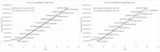
Figure 9.
Case 2: Cumulative total (left) and operating (right) costs with both CSPs and VSPs.
The payback period is 7 years, because the difference between the cumulative total costs is of 546,401.3 USD given that, in order to pay the initial loan in 10 years, a total of 531,009.53 USD is required. In this case, the price of the VSDs can be considered justified despite the fact that the costs related to the three devices is much bigger than in Case 2. However, money saved by employing these devices on the existing pumping system lead to a considerable reduction in the energy consumption during the year, shortening the payback period of the VDSs.
From the results obtained in this case, it is possible to state that the more powerful the pumping system is, the shorter the payback time required to repay the initial loan for the purchase and installation of VSDs is. However, more investigation is needed to confirm the latter outcome. It is worth noting that the pumping systems considered within this work are assumed to already exist, and that the original pumps are retained. If the pumping system was redesigned (meaning that the pumps were changed), VSDs could be more economically convenient. Indeed, in this case, the designer would have the opportunity to choose different pumps, allowing lower relative speeds (typically from one to a minimum speed of 0.5) than 0.85/0.8 (as in the present cases of study). Therefore, the pumps would absorb less power (as can be seen from Equation (9)), implying less energy and maintenance costs. However, this would also imply higher costs for the purchase and installation of new pumps.
4. Conclusions
Saving energy is one of the main goals of all industries, and water pumping systems are proven to be one of the most energy-consuming activities. Therefore, the use of an optimal regulation technique is of great importance in order to reduce energy consumption, with beneficial effects in terms of both economical savings and environmental protection. In this paper, the optimal regulation of an existing pumping system with constant speed pumps (CSPs) and variable speed pumps (VSPs) has been performed. The solutions provided by the two techniques have been compared from both technical and economical points of view. The use of variable speed drives (VSDs) helps to reduce the yearly operating costs (the sum of energy, maintenance and repair costs of the pumping systems), but introduces an additional cost related to the annual installments in order to pay back the initial loan. Therefore, the payback time of the VSDs has been estimated under the assumption that the pumping systems already exist; thus, only the costs for purchasing and installing the VSDs are added to the total yearly costs. From the results obtained, it could be concluded that the savings in the operating costs obtained by employing VSPs do not always justify the costs of the VSDs. In particular, for low-power pumping stations, employing an optimal schedule strategy based on VSPs seems to be less convenient than in the case of more powerful pumping systems. As a consequence, if one chose to employ VSDs in designing pumping stations, attention must be paid to the economical aspect to determine whether or not the price that must be paid for such devices is justified by the savings in energy and management costs. However, the use of VSDs leads to huge energy savings with respect to the case of the ON/OFF switch regulation of constant speed pumps, which, in turn, help to decrease the energy demand and lower the carbon emissions into the atmosphere. For this reason, the results obtained in this paper may change in favor of the use of VSDs if environmental aspects are introduced, even when such devices are not justified economically.
Author Contributions
Conceptualization, L.C. and C.C.; methodology, C.C.; software, L.C.; validation, B.M., and D.P.; formal analysis, L.C.; investigation, C.C.; resources, B.M.; data curation, B.M.; writing—original draft preparation, L.C.; writing—review and editing, C.C.; visualization, D.P.; supervision, D.P.; project administration, B.M. All authors have read and agreed to the published version of the manuscript.
Funding
This research received no external funding.
Conflicts of Interest
The authors declare no conflict of interest.
Nomenclature
amortization rate | |
total cost of energy | |
energy price during the i-th time interval | |
costs for maintenace and repair | |
operational costs | |
costs for purchase and installation of variable speed drives (VSDs) | |
total cost during the y-th year | |
water level within the r-th tank during the i-th time interval | |
minimum water level of the r-th tank | |
maximum water level of the r-th tank | |
initial water level of the r-th tank | |
head of the j-th pump at the characteristic rotational speed | |
head of the j-th pump during the i-th time interval | |
number of switch on of the j-th pump | |
maximum number of switch on allowed for the j-th pump | |
power absorbed by the j-th pump at its characteristic speed | |
power absorbed by the j-th pump at the i-th time interval | |
pumped discharge of the j-th pump at its characteristic rotational speed | |
pumped discharge of the j-th pump at the i-th time interval | |
relative rotational speed of the j-th pump at the i-th time interval | |
minimum relative rotational speed | |
specific weight of water | |
efficiency of the j-th pump during the i-th time interval |
References
- Lam, K.L.; Kenway, S.; Lant, P. Energy use for water provision in cities. J. Clean. Prod. 2017, 143, 699–709. [Google Scholar] [CrossRef]
- Karassik, I.J.; Messina, J.P.; Cooper, P.; Heald, C.C. Pump Handbook; McGraw-Hill: New York, NY, USA, 2001. [Google Scholar]
- Pasha, M.F.K.; Lansey, K. Strategies to Develop Warm Solutions for Real-Time Pump Scheduling for Water Distribution Systems. Water Resour. Manag. 2014, 28, 3975–3987. [Google Scholar] [CrossRef]
- Zhang, K.; Zhao, Y.; Cao, H.; Wen, H. Multi-scale water network optimization considering simultaneous intra- and inter-plant integration in steel industry. J. Clean. Prod. 2018, 176, 663–675. [Google Scholar] [CrossRef]
- Goldman, F.E.; Mays, L.W. The application of simulated annealing to the optimal operation of water systems. In Proceedings of the 26th Annual Water Resources Planning and Management Conference, Tempe, AZ, USA, 6–9 June 2000. [Google Scholar]
- López-Ibáñez, M.; Prasad, T.D.; Paechter, B. Ant Colony Optimization for Optimal Control of Pumps in Water Distribution Networks. J. Water Resour. Plan. Manag. 2008, 134, 337–346. [Google Scholar] [CrossRef]
- Savic, D.; Bicik, J.; Morley, M.S. A DSS generator for multiobjective optimisation of spreadsheet-based models. Environ. Model. Softw. 2011, 26, 551–561. [Google Scholar] [CrossRef]
- Candelieri, A.; Perego, R.; Archetti, F. Bayesian optimization of pump operations in water distribution systems. J. Glob. Optim. 2018, 71, 213–235. [Google Scholar] [CrossRef]
- Luna, T.; Ribau, J.; Figueiredo, D.; Alves, R. Improving energy efficiency in water supply systems with pump scheduling optimization. J. Clean. Prod. 2019, 213, 342–356. [Google Scholar] [CrossRef]
- Hashemi, S.S.; Tabesh, M.; Ataeekia, B. Ant-colony optimization of pumping schedule to minimize the energy cost using variable-speed pumps in water distribution networks. Urban Water J. 2013, 11, 335–347. [Google Scholar] [CrossRef]
- Nowak, D.; Krieg, H.; Bortz, M.; Geil, C.; Knapp, A.; Roclawski, H.; Böhle, M. Decision Support for the Design and Operation of Variable Speed Pumps in Water Supply Systems. Water 2018, 10, 734. [Google Scholar] [CrossRef]
- Abdallah, M.; Kapelan, Z. Fast Pump Scheduling Method for Optimum Energy Cost and Water Quality in Water Distribution Networks with Fixed and Variable Speed Pumps. J. Water Resour. Plan. Manag. 2019, 145, 04019055. [Google Scholar] [CrossRef]
- Mala-Jetmarova, H.; Sultanova, N.; Savic, D. Lost in optimisation of water distribution systems? A literature review of system operation. Environ. Model. Softw. 2017, 93, 209–254. [Google Scholar] [CrossRef]
- Makaremi, Y.; Haghighi, A.; Ghafouri, H.R. Optimization of Pump Scheduling Program in Water Supply Systems Using a Self-Adaptive NSGA-II; a Review of Theory to Real Application. Water Resour. Manag. 2017, 31, 1283–1304. [Google Scholar] [CrossRef]
- Bloch, H.P.; Budris, A.R. Pump User’s Handbook: Life Extension; Fairmont Press: Lilburn, GA, USA, 2004. [Google Scholar]
- Saidur, R.; Mekhilef, S.; Ali, M.; Safari, A.; Mohammed, H.A. Applications of variable speed drive (VSD) in electrical motors energy savings. Renew. Sustain. Energy Rev. 2012, 16, 543–550. [Google Scholar] [CrossRef]
- Lansey, K.E.; Awumah, K. Optimal Pump Operations Considering Pump Switches. J. Water Resour. Plan. Manag. 1994, 120, 17–35. [Google Scholar] [CrossRef]
- Cimorelli, L.; Morlando, F.; Cozzolino, L.; D’Aniello, A.; Pianese, D. Comparison Among Resilience and Entropy Index in the Optimal Rehabilitation of Water Distribution Networks Under Limited-Budgets. Water Resour. Manag. 2018, 32, 3997–4011. [Google Scholar] [CrossRef]
- Cimorelli, L.; D’Aniello, A.; Cozzolino, L. Boosting Genetic Algorithm Performance in Pump Scheduling Problems with a Novel Decision-Variable Representation. J. Water Resour. Plan. Manag. 2020, 146, 04020023. [Google Scholar] [CrossRef]
- Rossman, L.A. EPANET 2: Users Manual; U.S. Environmental Protection Agency: Cincinnati, OH, USA, 2000.
- Van Zyl, J.; Savic, D.; Walters, G. Operational Optimization of Water Distribution Systems Using a Hybrid Genetic Algorithm. J. Water Resour. Plan. Manag. 2004, 130, 160–170. [Google Scholar] [CrossRef]
- De Paola, F.; Fontana, N.; Giugni, M.; Marini, G.; Pugliese, F. An Application of the Harmony-Search Multi-Objective (HSMO) Optimization Algorithm for the Solution of Pump Scheduling Problem. Procedia Eng. 2016, 162, 494–502. [Google Scholar] [CrossRef]
- Rao, Z.; Salomons, E. Development of a real-time, near-optimal control system for water-distribution networks. J. Hydroinform. 2007, 9, 25–38. [Google Scholar] [CrossRef]
- De Marchis, M.; Milici, B.; Volpe, R.; Messineo, A. Energy Saving in Water Distribution Network through Pump as Turbine Generators: Economic and Environmental Analysis. Energies 2016, 9, 877. [Google Scholar] [CrossRef]


© 2020 by the authors. Licensee MDPI, Basel, Switzerland. This article is an open access article distributed under the terms and conditions of the Creative Commons Attribution (CC BY) license (http://creativecommons.org/licenses/by/4.0/).