Abstract
Atmospheric stability has been studied for decades. There are several methodologies that evolved over the years. In this study, a special experimental meteorological mast that has been erected to a complex site has been used to calculate dimensionless Obukhov length (, dimensionless momentum (), and heat coefficients (). The results are compared with the ones from average value approaches: Richardson number, flux-profile (F-P) relations, and wind shear exponent methods. The results show that the estimated values, using the bulk Richardson number, get along well with the reference within the neutral and stable regimes. F-P relations and wind shear exponent methods result in the best agreement for stable and neutral regimes. Nevertheless, average oriented methods are not reliable for the other regimes.
1. Introduction
The boundary layer theory dates back to the 19th century and is used in topics related to the motion of the fluids such as atmospheric boundary layer, distinctive properties of turbulence, and eddies. In order to obtain the necessary parameters of the boundary layer characteristics, a measurement campaign is crucial. In the current decade, data collection is made either through a conventional meteorological mast or new generation remote sensing tools (e.g., Lidars). The data processing is performed to calculate values such as Monin–Obukhov length, heat flux, Richardson number, flux-profile functions, and so on. It is known that thermal and mechanical forces affect the eddy motion—which determines the thickness of the atmospheric boundary layer, studied by [1]. Halstead considers logarithmic wind velocity profile (maximum at ground and minimum at boundary layer (BL) thickness) for the different lapse rates and obtains a stability term for the velocity profile [2]. Holzman investigated the effect of stability on evaporation and coined an expression using Prandtl’s mixing length approach to calculate it [3]. Monin and Obukhov used mixing length height to represent surface layer (SL) height since, in their approach, L is obtained by using constant flux assumption. They also prove that Richardson number gradient goes to the same value with inverse Obukhov length on the ground. Deriving Austausch coefficient for different types of temperature conditions, which is used for presenting wind shear and heat rate, they showed that it depends on the mixing height and Richardson number [4]. Knowing that Richardson number is a function of stability and roughness, the authors suggested so many relations [5,6,7,8,9,10,11,12,13,14,15,16,17]. The difference between those given studies lies in the location where the study is carried out, since the type of the field and wind profile of the given locations differ from each other, and the coefficient of the empirical relations does too. However, it can be concluded that the degree of the proposed equations is the same for most of them. Usage of the different types of sensors increased with time. The authors revealed that sonic temperatures differ from those obtained by the thermocouples [18,19,20,21]. Schotanus proposed that heat and moisture variables can be obtained by using sonic anemometers by applying the Bowen ratio and energy balance method. Kaimal and Gaynor derived sonic and virtual temperature equations where corrections are based on horizontal wind speed, vapor pressure of water, and absolute pressure.
In this study, a comparison between estimated by using Monin-Obukhov similarity theory (MOST) and Richardson number and wind shear exponent is given. In literature, similar works are carried out by [22,23,24,25], and it seems that, depending on the terrain, different results may be obtained. Wind shear exponent is another way to find stability classes, by [26,27,28,29], where only wind speed measurements are available.
The stability analysis concept hinges on two parameters: scaled velocity and temperature profile. Air motion is upward if the dominant force is buoyancy, while vertical motion is strongly damped out under extreme stability condition and moves horizontally within the inversion. Using both velocity and temperature scales, Obukhov length is used as a criterion of the air stability. Since the 3D measurements may be unavailable at any field study, 2D measurements should be performed for an analysis: Richardson method, wind shear exponent, flux-profile (F-P) relation, etc. Using the data from the previously installed masts equipped with the only cup anemometers and wind vanes (vertical velocity, temperature gradient, and humidity are absent), those approaches to perform stability are biased. However, these sorts of approaches provide benefits of the data. In this study, we performed the Monin–Obukhov similarity theory, MOST, for the 12-month measurement campaign and compared the mixing lengths obtained by the Richardson method. The aim was to carry out MOST on complex terrain, since it has been mostly performed on flat terrain (Høvsøre, KANSAS, Arctic Ocean data sets). Roughness affects the speed and temperature profile near the surface; and the diabatic factor, used in logarithmic wind profile equation, becomes the function of roughness and length scale near the surface or on the surface. Performing the analysis only for flat terrain, bias is expected for the complex terrain. Lastly, we obtained the consistent ranges of stability to perform Richardson or wind shear exponent methods for the given complex terrain.
1.1. MOST with Three-Dimensional High Frequency Data
Monin–Obukhov Similarity Theory, MOST, is one of the most common theories such as Mixed-Layer similarity, Local similarity, Rossby-Number similarity, and so on. It is restricted by the surface layer, since further Mixed-Layer and other theories are valid. It depends on constant flux approximation, that is, flux values vary up to 10% of their magnitudes [30]. Stability term, , function of the height and dimensionless Obukhov length, used for estimating velocity, is a crucial parameter since it links L to the velocity profile. To find length scale, no matter if it is surface, mixed, or convective, one should use an appropriate empirical formula and calculate it [4,16,31]. The Monin–Obukhov length is calculated as
where is friction velocity and calculated as . is buoyancy term where T is temperature. In addition, is the basis for the vertical heat flux, where is virtual potential temperature and w is vertical component of the velocity. Virtual potential temperature is obtained by using or formula depending on the air saturation. r terms are related with the air–water ratio, so that, and are water-vapor saturation mixing ratio and liquid water mixing ratio, respectively [30].
We used several types of sensors, given in Table 1, to estimate L, Richardson and other parameters for comparison. For the sake of the aim, we perform different types of methods: estimating directly by using sonic measurements, using Richardson method, Flux–Profile relations, and wind shear. We chose MOST as the reference method since it is the most comprehensive theory compared to the others. Vertical component of the velocity can be taken by sonic anemometers. On the other hand, sonic anemometers are deficient in not measuring the humidity to calculate virtual potential temperature. The authors suggest corrections in terms of humidity and the crosswind factors [18,32,33].

Table 1.
IZTECH 100 m met mast properties.
1.2. Richardson Method
Richardson number has several types in terms of usage, flux, gradient, and bulk Richardson number. Ri number is very important since it can be used for determining the status of the flow, whether the flow will be laminar or turbulent; and it relates with [16], which can be used in Pasquill and Turner classification systems. Here, we used Bulk Richardson number, calculated as [30],
where , since velocity is zero at aerodynamic roughness height (where the velocity is zero). , which can be approximated as . , where the virtual potential temperatures are measured at and . The Richardson method enables us to use an empirical relation to find [16], such as
where there are many suggested and values in literature such as 0.74 for , 10 for [5,16], and so on. Equations (3) and (4) are used for negative and positive numbers, respectively [16]. We used 10 and 5 for and , as in [24]. These values are studied by many researchers; and the findings are as follows: is estimated as 12 for the stability ranges between −0.012 and 0.012, by [34]. In a different study, was calculated as 6.78, where , while it is 10.89 where [35]. and values are suggested to be and [36]. Since Grachev’s study was made on the sea surface and our terrain is complex, suggested values yield to the errors for values in our study.
1.2.1. Flux-Profile Relations
Dimensionless wind shear, , dim-less lapse rate, , and dim-less humidity gradient, are terms used in similarity studies valid under the surface layer. and are used for linking Richardson number and , in a way that [5]
where is eddy diffusivity ratio, . The name of the profile comes from the shape of the data distribution, where: depending on the stability region, its shape is approximated as those said profile functions. Dimensionless wind shear can be expressed as , while dim-less lapse rate is expressed as under unstable air condition, where and are the fitted parameters of the case studies. For the stable region, both of them were stated by a linear formula. Other expressions, such as and that is constant, are also suggested [5,17]. In a SHEBA case study, profile functions are stated as power of values for the extreme cases [12]. It concluded that , are for very extreme cases. Integrating and universal stability term, , is obtained, which is the key parameter merging profiles (velocity and temperature) and air stability.
1.2.2. Wind Shear Method
A wind shear exponent is found by performing a power-law assumption in which wind velocity changes with vertical height exponentially, that is,
where m stands for the wind shear exponent. Here, anything related with heat is out of the equation, but it is known that stability affects velocity. Therefore, how much this equation works is a good question. There are studies which links the wind shear exponent with surface roughness and the stability term [26,27,37,38,39]. The wind shear exponent, m, is used for categorizing air stability depending on its range [40,41], and the last study is the one which shows the Ri number and shear exponent relation [27]. In the following table, a summary of that aforementioned parameter is given.
A more detailed table can be found in [42] where stability classes are compared by using , wind shear exponent, and SODAR stability parameters (turbulent kinetic energy, TKE, and turbulent intensity, I).
2. Experimental Setup
IZTECH 100 m meteorological mast has been founded where the coordinates are N and E, given in Figure 1. The elevation from the sea level is 52 m, and the location area of the meteorological mast is steeper, so it is not flat terrain. Measurement data were collected from December 2017 to December 2018. The sampling rate of the mast is 1 Hz, and the equipment is shown in Table 1.
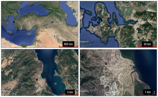
Figure 1.
The location of the IZTECH met mast.
Figure 1 reveals the location of the study from different scales. Table 1 shows the mounted equipment, mast’s properties, and sensor heights.
There are four cup anemometers, two ultrasonic sensors, three wind vanes, three humidity/temperature sensors, and two pressure sensors on the mast. Depending on the sensor height and sensor type, boom and rod geometries vary. Orientation angle also varies for each sensor; and its adjustments are made by considering rod and boom, which distort the airflow.
3. Results
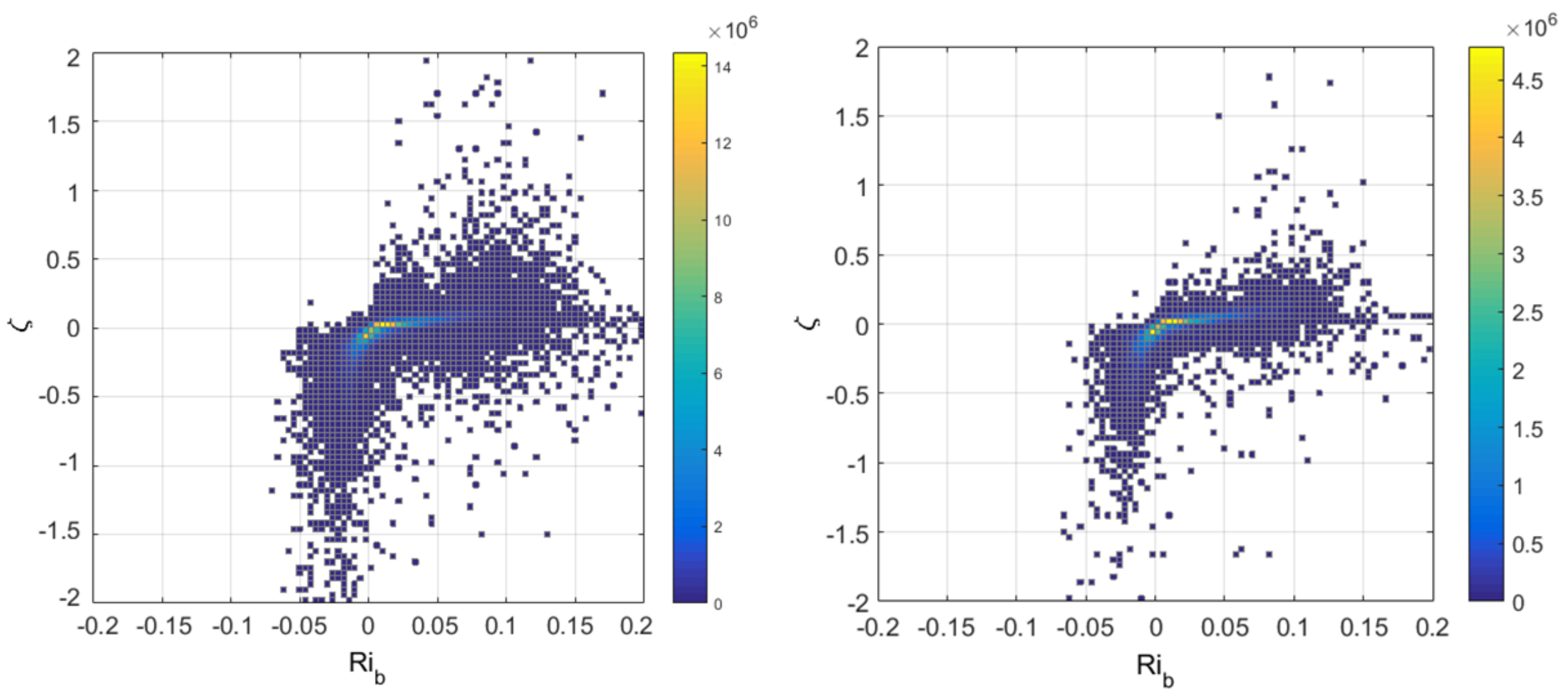
In this study, we performed several types of approaches to estimate such as direct measurements of fluxes by using ultrasonic sensors, by using bulk Richardson number, and parameters, and wind shear exponents. MOST with the ultrasonic measurements gives the best results, so it is selected as a reference. Firstly, and distribution is shown in Figure 2. This histogram emphasizes the pattern of these two parameters for the limited range—to avoid extreme cases. was applied for the . The bin color is related to data frequency (the lighter it becomes, the more frequent it becomes). Since the time scale is a distinctive feature for turbulent fluxes, we performed the analyses for two different cases (10 min and 30 min).
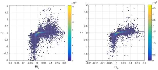
Figure 2.
Distribution of and for two different time scales of 10 min (to the left) and 30 min (to the right).
Most of the data distributed linearly in the neutral regions is given in and scattered as the instability increases, which is the same in both cases. values are put in Equations (3) and (4); and empirical results are obtained, as shown in Figure 3. As another fitting parameter, m and n values can be obtained for our study, which enables us to check if it gives similar results for the other sites with similar geologic conditions. Figure 2 shows the distribution of and . Yellow segments are the densest parts located near zero where linear characteristics can be observed. A quadratic relation takes place for the stable part up to 0.2, which is a critical point of .
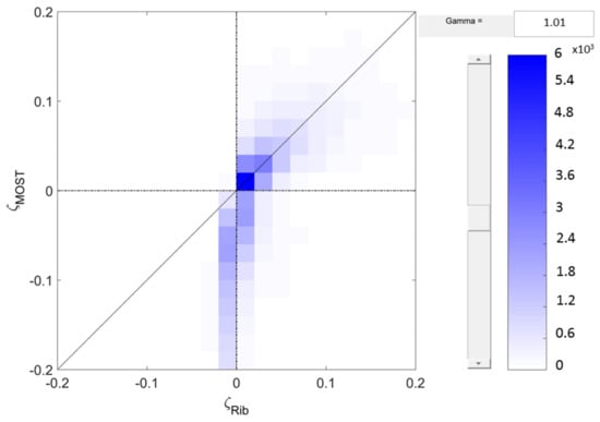
Figure 3.
evaluated by direct measurements and obtained from averaged values compared directly.
Gamma is to adjust the blur and color density directly related to the data collection. We calculated by using empirical formulae in between of [−0.2, 0.2], as our findings disagree with the reference values by the increasing instability. This figure shows the coherence of two parameters where the is underestimated in unstable and very unstable regions—which resulted from the temperature difference and humidity—while both parameters get along well between neutral and stable regions.
Figure 4 shows the distribution of the sensible heat flux at 10 m. In both illustrations, similarity mostly occurs in between stable and neutral regions, whereas there is an inconsistency for the positively sensible heat fluxes. In an unstable part of the left graph, near the neutral region, a scatter of the is small, while the opposite type of distribution is observed in the unstable zone. In the second figure on the right, it shows that a little change in the negative can result in a quite large change in the sensible heat flux and a sudden of increment in observed values in the convective zone. In MOST, kinematic fluxes are nothing but a covariance of the velocity and temperature parameters. The same method is used when the friction velocity wants to be found. In the following, how the friction velocity is distributed, depending on the stability, is given.
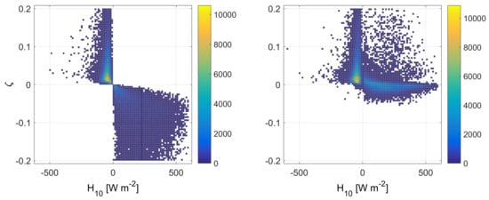
Figure 4.
Comparison of the sensible heat fluxes obtained with MOST and , respectively.
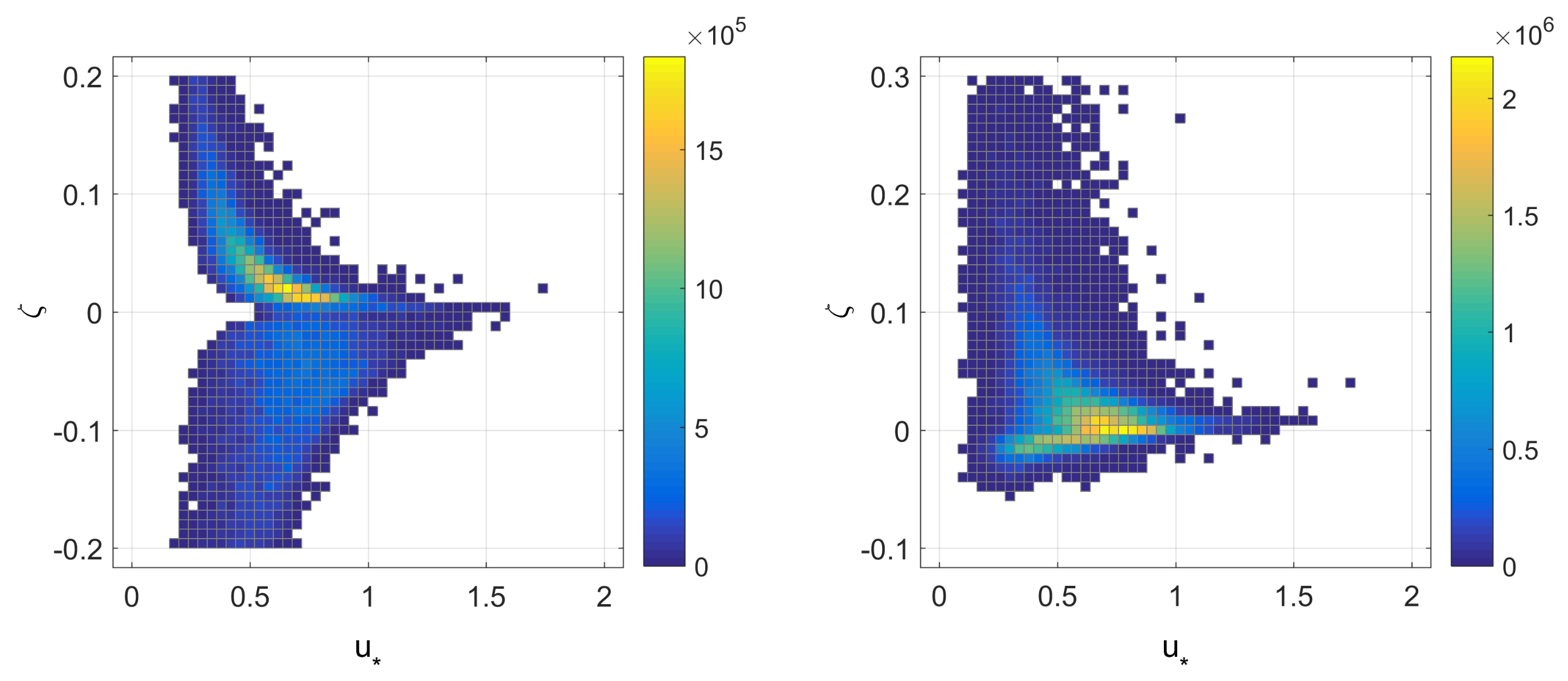
How the friction velocity is affected by stability can be seen in Figure 5. Both figures agree with the results that friction velocity becomes maximum in a neutral region and gets smaller under the instability conditions. The most frequent value of the is found as and in MOST and , respectively. It can be observed that, after a near-neutral region, the distribution doesn’t continue within the unstable region in Figure 5 (right). However, both figures show the same characteristics within stable and neutral regions. Particularly, in the near-neutral region, the most recurrent value is almost identical for both of them. Even it is given as and near , the range of distribution is quite large with respect to the rest of the values, which shows that the covariance of kinematic flux reach their maximum here. In addition, all of the velocity components vary on a large scale, where can reach almost 2 m/s. In the convective layer, the vertical velocity becomes dominant, and horizontal components get undetectable by increasing upward air motion. Thus, the covariances of the parameters also get decreased and result in small . The same tendency occurs within the stable regime where the horizontal components are much larger than the vertical speed component, which takes us to the same result of finding small values. The additional observation is as given previously; the distribution ends in a near-neutral or weak convective regime where the is near –0.05 estimated by . This fact enables us to say that the suggested method can detect an unstable region up to the weak convective layer that ends near . However, both methods give a very similar distribution pattern up to that point. can also be used in estimation of the profile functions that are dimensionless momentum and heat parameters, and . All of these parameters mentioned are linked to each other by empirically, Equation (5). If the velocity and temperature gradients are known, dimensionless momentum and heat can be calculated. To calculate those parameters, we use wind speed and temperature gradients, as given in [8].

Figure 5.
and distribution for two different approaches. was calculated with MOST on the (left) and on the (right) illustration.
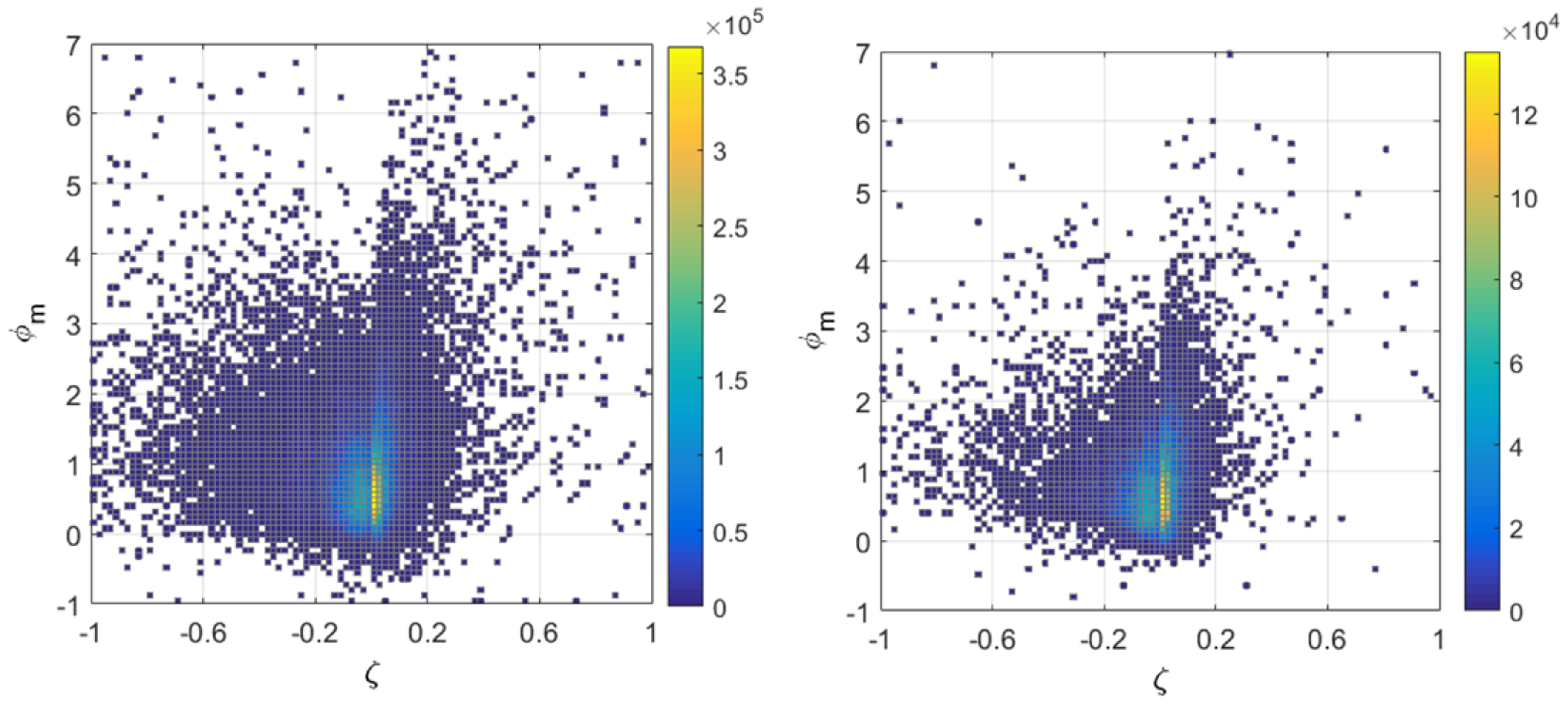
Figure 6 contains our samples as 10 min of means and discretized values. Comparing the discretized samples with the Businger and Höngström profiles, we see that the biggest difference occurs in the unstable region again. On the other hand, they get along well up to the very stable region. We also looked at the histogram of the and to see the distribution of the parameters for two different time periods (10 min and 30 min).
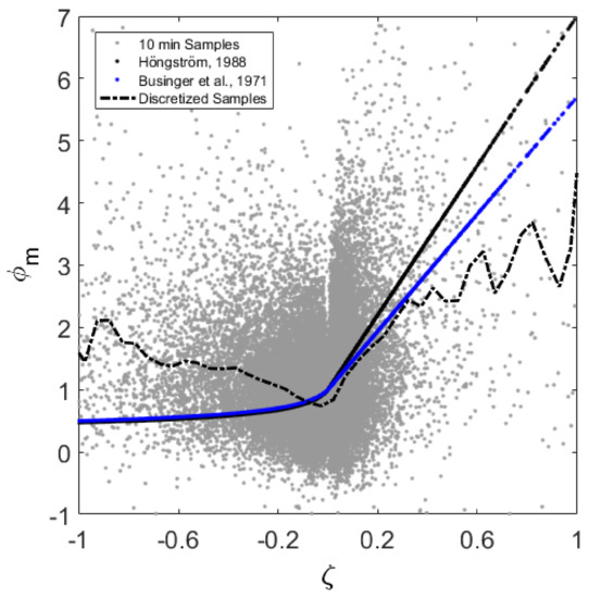
Figure 6.
and relation with a comparison of theoretical values.
It is not enough to show the relationship between and with only average values since extreme values can alter the results even when their frequency is small. Therefore, Figure 7 provides a more insightful perspective by giving the distribution of the two parameters for two different time scales. It reveals that is collected between zero and one as the goes to zero for both time scales. Another observation is that values increase much rapidly within the stable region compared to the unstable one in both time scales. The wind shear exponent is one of the recommended methods, and can be used when the temperature measurements are not available. Exponential parameter is calculated between 10–52 m and 30–76 m, and is compared to for 30 min samples.

Figure 7.
Distribution of the and by using two different time scales of 10 min and 30 min, respectively.
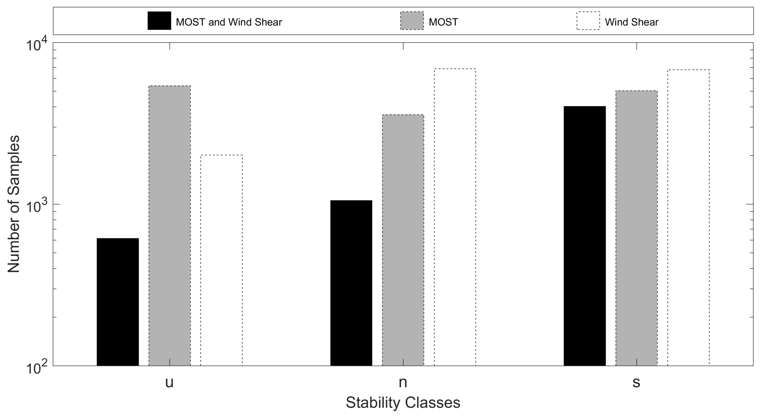
Figure 8 shows that m distributed between 0 and 0.2 in very unstable (convective) regions according to the first plot on the left, but there isn’t a similar behavior in the other one. The abrupt change in the pattern originated by jet stream at 52 m. As the goes to 0, mostly recurrent values occur near 0.2. The patterns differ according to their length and density in both figures, despite their similarity. There are conflicts among the samples where the negative m values are expected on the left side of the short dashed line. To see more clearly, we collected all the bins according to their limits and made another comparison, given in Figure 9. Black bars stand for the agreement of both methods, while gray and white ones with dashed lines represent MOST and wind shear exponent, respectively.
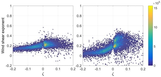
Figure 8.
and wind shear exponent (m) distribution for 30 min samples.

Figure 9.
Comparison of the two different types of stability classification methods.
In the unstable regime, a shear exponent underestimates the sample numbers with respect to the MOST and the agreed number of the samples by both methods near 600. The MOST underestimates the sample number in the neutral regime where the agreed number is 1000. The agreement within the neutral regime is higher than the one from an unstable regime. Final regime, stable region, gives the most consistent results for both methods. The sample number from both methods’ intersection is almost equal to the ones obtained by MOST. Figure 9 gives all the sample numbers where the density is not take into account. Thus, depending only on this illustration and making a judgement is not easy. Even the observations in Figure 9 show disagreement in the neutral region; this is originated by not considering the frequency again. On the contrary, Figure 8 indicates that the densest part of the distribution is located near the zero. Therefore, both of the Figure 8 and Figure 9 are used to conclude that a shear exponent can be used in stability analysis within the neutral and stable regimes.
4. Discussion
All of the stability related parameters (, , , and m) have been investigated among different stability regions. However, extreme instability conditions are generally excluded in results by the reason of inadequacy of MOST. It is observed that upward heat flux is the most crucial phenomenon for a convective regime. To filter our results, sensible heat fluxes in the range of [−10, 10] [W m] were excluded, since it is not possible to detect those fluxes accurately in that given range. In the unstable regime, vertical disturbances occur, different characteristic air layers are mixed and finally cease. When this disturbance fades away, our findings agree well with those in the literature [8,25,35,40,42]. and distribution have a similar pattern to those within the literature for a restricted region [25,30]. Nevertheless, the density gradually decreases as the instability increases, especially in the unstable region. Time intervals also have an effect on the sample distribution, as given in Figure 2. In addition, a 30 min time scale produces less scattered distribution, by capturing the larger scale of the parameters, with respect to the other one. After calculating empirical , consistency couldn’t be obtained in the unstable region. Virtual temperature differences between two altitudes result in this miscalculation because of those measurements produced by a temperature/humidity sensor at 3 m and a sonic at 10 m. Corrections are made for the sonic temperatures by using the principles from [18,21]. Sensible heat flux is calculated by using the covariance of the vertical speed and virtual potential temperature. A large scatter is observed in Figure 4 (right), since the used in evaluation of . It has been shown that bulk heat flux is inadequate for estimating for the convective regime [25]. However, almost identical distribution is observed in the neutral and stable regimes. Kinematic heat and momentum fluxes can be easily affected from surface characteristics (roughness). If the range of measured values vary on a large scale in the reference time scale (10 min or 30 min), their fluctuations also show the same behavior that resulted in big covariance values for the momentum and heat fluxes. The biggest range of the is observed in a neutral regime. For the dimensionless momentum and heat parameters, discretized samples—to represent those points with their mean—are compared to well-known profiles. Here, there is an increment in the in the convective region, which was expected to become constant. Therefore, looking at only Figure 6 would be a mistake in terms of comparison. A histogram of these two parameters enable us to make a better comparison by revealing the frequency of the samples. Contrary to scatter plot, Figure 7 shows the rapid change of in the stable region. The densest part of the is the range of [0, 1] where, depending on the time interval, density varies. The weighted average of the samples should be used rather than the average values which are altered by extreme points easily. Figure 7 puts forward the importance of the samples density. The final suggested method, wind shear exponent, has reached very extreme stability conditions. Reliability reaches the higher shear exponents in the 2nd plot at the right side of the Figure 8. In the restricted area between [−0.2, 0.2], the densest part of the distribution exists. Both of the methods point at the same stability classes as the density increases. Critical m value was given as 0.2 for the neutral region in Table 2, where the highest frequency exists also for the . Figure 9 gives a measure of consistency between the shear exponent and , where the best scenario is that a shear exponent works well under neutral conditions. The conflict happens mostly under the very stable regime, which is even worse than the convective regime. Here, the questions of where all the suggested empirical relations work, and under which classes, are answered. For a complex site with similar geologic conditions to ours, reliability and limitations for the parameters are investigated. The critical point is that the vertical heat motion dominates the findings, and it has to be corrected as much as possible.

Table 2.
Stability classification with wind shear exponent [40].
5. Conclusions
The question of how to make benefits from the data coming from the conventional meteorological mast has always been important. Average value-oriented approaches from the literature are applied to the time-series obtained by our measuring campaign. The reason for doing that was to see whether average-oriented methods give favorable results in a complex site. All given approaches are insufficient in the convective layer due to the domination of the vertical disturbances in the region. Both the Richardson and wind shear exponent methods underestimate the in that region, while the dimensionless velocity, , is overestimated. The distribution of and shows that the densest parts are in good agreement with the ones from literature [5,8]. The principal for obtaining profile functions is well explained in [8] and also used in this study. Friction velocity and velocity gradient affect the and a large scatter of the is produced. Unlikely, in the stable regime, both the means and frequency agree well with the reference profiles [5,8] up to the very stable regime. Another underestimation is done in the very-stable zone using the wind shear exponent. For the dimensionless momentum, values are higher than the ones from the literature, which yields a different pattern. Histograms, which are prepared considering two different time scales, provide a better understanding of the distribution of the parameters and fix the mismatch given in the previous sentence. Thus, using the weighted average of the distribution eliminates the effect of the extreme values. The scenario at the beginning (providing benefits from the data obtained in the absence of new generation measurement tools) becomes real under those conditions where the stability classes are: neutral and stable. Reliability of these aforementioned methods can also be seen in our results.
Author Contributions
All authors have read and agree to the published version of the manuscript. Conceptualization, F.B.; methodology, F.B.; validation, F.T.; formal analysis, F.T.; investigation, F.B and F.T.; resources, F.B.; data curation, F.T.; writing–original draft preparation, F.B. and F.T.; visualization, F.T.; supervision, F.B.; project administration, F.B.; funding acquisition, F.B. All authors have read and agreed to the published version of the manuscript.
Funding
Funded by the Scientific and Technological Research Council Of Turkey (TÜBITAK); 215M384.
Acknowledgments
This project has been a part of the ERANET+ project, the New European Wind Atlas (NEWA). We would like to thank to our project partners for the collaboration and the Scientific and Technological Research Council Of Turkey (TÜBITAK) for funding our project.
Conflicts of Interest
The authors declare no conflict of interest.
References
- Taylor, G.I. Statistical theory of turbulence. Proc. R. Soc. Lond. Ser. A Math. Phys. Sci. 1935, 151, 421–444. [Google Scholar] [CrossRef]
- Halstead, M. A stability-term in the wind-gradient equation. Eos Trans. Am. Geophys. Union 1943, 24, 204–208. [Google Scholar] [CrossRef]
- Holzman, B. The influence of stability on evaporation. Ann. N. Y. Acad. Sci. 1943, 44, 13–18. [Google Scholar] [CrossRef]
- Monin, A.; Obukhov, A. Basic laws of turbulent mixing in the surface layer of the atmosphere. Contrib. Geophys. Inst. Acad. Sci. USSR 1954, 151, e187. [Google Scholar]
- Businger, J.A.; Wyngaard, J.C.; Izumi, Y.; Bradley, E.F. Flux-profile relationships in the atmospheric surface layer. J. Atmos. Sci. 1971, 28, 181–189. [Google Scholar] [CrossRef]
- Grachev, A.A.; Andreas, E.L.; Fairall, C.W.; Guest, P.S.; Persson, P.O.G. The critical Richardson number and limits of applicability of local similarity theory in the stable boundary layer. Bound.-Layer Meteorol. 2013, 147, 51–82. [Google Scholar] [CrossRef]
- Sorbjan, Z.; Grachev, A.A. An evaluation of the flux–gradient relationship in the stable boundary layer. Bound.-Layer Meteorol. 2010, 135, 385–405. [Google Scholar] [CrossRef]
- Högström, U. Non-dimensional wind and temperature profiles in the atmospheric surface layer: A re-evaluation. In Topics in Micrometeorology. A Festschrift for Arch Dyer; Springer: New York, NY, USA, 1988; pp. 55–78. [Google Scholar]
- Yang, K.; Tamai, N.; Koike, T. Analytical solution of surface layer similarity equations. J. Appl. Meteorol. 2001, 40, 1647–1653. [Google Scholar] [CrossRef]
- Dellwik, E.; Jensen, N.O. Flux–profile relationships over a fetch limited beech forest. Bound.-Layer Meteorol. 2005, 115, 179. [Google Scholar] [CrossRef]
- Grachev, A.; Fairall, C.; Bradley, E. Convective profile constants revisited. Bound.-Layer Meteorol. 2000, 94, 495–515. [Google Scholar] [CrossRef]
- Grachev, A.A.; Andreas, E.L.; Fairall, C.W.; Guest, P.S.; Persson, P.O.G. SHEBA flux–profile relationships in the stable atmospheric boundary layer. Bound.-Layer Meteorol. 2007, 124, 315–333. [Google Scholar] [CrossRef]
- Byun, D.W. On the analytical solutions of flux-profile relationships for the atmospheric surface layer. J. Appl. Meteorol. 1990, 29, 652–657. [Google Scholar] [CrossRef]
- Arya, S. Parametric relations for the atmospheric boundary layer. Bound.-Layer Meteorol. 1984, 30, 57–73. [Google Scholar] [CrossRef]
- Foken, T.; Skeib, G. Profile measurements in the atmospheric near-surface layer and the use of suitable universal functions for the determination of the turbulent energy exchange. Bound.-Layer Meteorol. 1983, 25, 55–62. [Google Scholar] [CrossRef]
- Golder, D. Relations among stability parameters in the surface layer. Bound.-Layer Meteorol. 1972, 3, 47–58. [Google Scholar] [CrossRef]
- Dyer, A.; Hicks, B. Flux-gradient relationships in the constant flux layer. Q. J. R. Meteorol. Soc. 1970, 96, 715–721. [Google Scholar] [CrossRef]
- Schotanus, P.; Nieuwstadt, F.; De Bruin, H. Temperature measurement with a sonic anemometer and its application to heat and moisture fluxes. Bound.-Layer Meteorol. 1983, 26, 81–93. [Google Scholar] [CrossRef]
- Dias, N.; Gonçalves, J.; Freire, L.; Hasegawa, T.; Malheiros, A. Obtaining potential virtual temperature profiles, entrainment fluxes, and spectra from mini unmanned aerial vehicle data. Bound.-Layer Meteorol. 2012, 145, 93–111. [Google Scholar] [CrossRef]
- Liu, H.; Peters, G.; Foken, T. New equations for sonic temperature variance and buoyancy heat flux with an omnidirectional sonic anemometer. Bound.-Layer Meteorol. 2001, 100, 459–468. [Google Scholar] [CrossRef]
- Kaimal, J.; Gaynor, J. Another look at sonic thermometry. Bound.-Layer Meteorol. 1991, 56, 401–410. [Google Scholar] [CrossRef]
- Essa, K.S. Estimation of Monin–Obukhov length using Richardson and bulk Richardson number. In Proceedings of the Second Conference on Nuclear and Particle Physics (NUPPAC-99), Cairo, Egypt, 13–17 November 2000; Volume 711. [Google Scholar]
- Zoumakis, N.; Kelessis, A. On the theoretical relationship between the Monin–Obukhov stability parameter and the bulk Richardson number. Il Nuovo Cimento C 1993, 16, 1–7. [Google Scholar] [CrossRef]
- Peña, A.; Gryning, S.E.; Hasager, C.B. Measurements and Modelling of the Wind Speed Profile in the Marine Atmospheric Boundary Layer. Bound.-Layer Meteorol. 2008, 129, 479–495. [Google Scholar] [CrossRef]
- Peña, A.; Hahmann, A.N. Atmospheric stability and turbulence fluxes at Horns Rev—An intercomparison of sonic, bulk and WRF model data. Wind Energy 2012, 15, 717–731. [Google Scholar] [CrossRef]
- DeMarrais, G.A. Wind-speed profiles at Brookhaven National Laboratory. J. Meteorol. 1959, 16, 181–190. [Google Scholar] [CrossRef]
- Heald, R.; Mahrt, L. The dependence of boundary-layer shear on diurnal variation of stability. J. Appl. Meteorol. 1981, 20, 859–867. [Google Scholar] [CrossRef]
- Sutton, O. The problem of diffusion in the lower atmosphere. Q. J. R. Meteorol. Soc. 1947, 73, 257–281. [Google Scholar] [CrossRef]
- Touma, J.S. Dependence of the wind profile power law on stability for various locations. J. Air Pollut. Control Assoc. 1977, 27, 863–866. [Google Scholar] [CrossRef]
- Stull, R.B. An Introduction to Boundary Layer Meteorology; Springer Science & Business Media: New York, NY, USA, 2012; Volume 13. [Google Scholar]
- Gryning, S.E.; Batchvarova, E.; Brümmer, B.; Jørgensen, H.; Larsen, S. On the extension of the wind profile over homogeneous terrain beyond the surface boundary layer. Bound.-Layer Meteorol. 2007, 124, 251–268. [Google Scholar] [CrossRef]
- Burns, S.; Horst, T.; Jacobsen, L.; Blanken, P.; Monson, R. Using sonic anemometer temperature to measure sensible heat flux in strong winds. Atmos. Meas. Tech. 2012, 5, 2095–2111. [Google Scholar] [CrossRef]
- Kaimal, J.C.; Finnigan, J.J. Atmospheric Boundary Layer Flows: Their Structure and Measurement; Oxford University Press: Oxford, UK, 1994. [Google Scholar]
- Deardorff, J.W. Dependence of air-sea transfer coefficients on bulk stability. J. Geophys. Res. 1968, 73, 2549–2557. [Google Scholar] [CrossRef]
- Grachev, A.; Fairall, C. Dependence of the Monin–Obukhov stability parameter on the bulk Richardson number over the ocean. J. Appl. Meteorol. 1997, 36, 406–414. [Google Scholar] [CrossRef]
- Holtslag, M.; Bierbooms, W.; Van Bussel, G. Estimating atmospheric stability from observations and correcting wind shear models accordingly. In Journal of Physics: Conference Series; IOP Publishing: Bristol, UK, 2014; Volume 555, p. 012052. [Google Scholar]
- Panofsky, H.; Blackadar, A.; McVehil, G. The diabatic wind profile. Q. J. R. Meteorol. Soc. 1960, 86, 390–398. [Google Scholar] [CrossRef]
- Irwin, J.S. A theoretical variation of the wind profile power-law exponent as a function of surface roughness and stability. Atmos. Environ. 1979, 13, 191–194. [Google Scholar] [CrossRef]
- Essa, K.S.; Embaby, M.; Etman, S.M. A notional variation of the wind profile power-law exponent as a function of surface roughness and stability. In Proceedings of the 4th Conference on Nuclear and Particle Physics, Guildford, UK, 29–30 March 2004. [Google Scholar]
- Van den Berg, G. Wind turbine power and sound in relation to atmospheric stability. Wind Energy 2008, 11, 151–169. [Google Scholar] [CrossRef]
- Walter, K.; Weiss, C.C.; Swift, A.H.; Chapman, J.; Kelley, N.D. Speed and direction shear in the stable nocturnal boundary layer. J. Sol. Energy Eng. 2009, 131, 011013. [Google Scholar] [CrossRef]
- Wharton, S.; Lundquist, J.K. Assessing atmospheric stability and its impacts on rotor-disk wind characteristics at an onshore wind farm. Wind Energy 2012, 15, 525–546. [Google Scholar] [CrossRef]
© 2019 by the authors. Licensee MDPI, Basel, Switzerland. This article is an open access article distributed under the terms and conditions of the Creative Commons Attribution (CC BY) license (http://creativecommons.org/licenses/by/4.0/).


