An Evaluation Method of Brittleness Characteristics of Shale Based on the Unloading Experiment

Abstract

Shale reservoir has an initial unloading effect during the natural uplift and erosion process, which causes the shale brittleness to change, affecting the design of the fracturing scheme. To consider this, the axial compression loading and confining pressure unloading experiment of shale is carried out, and then the influence of unloading rate on the mechanical parameters, failure characteristics, and the brittleness of rock are analyzed. What is more, a new evaluation method of brittleness characteristics that take the unloading effect into consideration is proposed. The conclusions are as follows: (1) The unloading rate has a weakening effect on the mechanical parameters, such as the destructive confining pressure and the residual strength of the samples. (2) The failure characteristics of shale specimens are a single shear failure in an oblique section under low unloading rate, and multiple shear zones accompanied with bedding fracture under high unloading rate. (3) The brittleness of shale samples is well verified by the brittleness index $B_{d1}$ and $B_{d2}$ during the loading path; nevertheless, it has shortage at the unloading path. This paper proposes a new brittleness evaluation method which can consider the influence of the different unloading rates and unloading points. Furthermore, there is a nice characterization between the brittleness damage and this method.

1. Introduction

In recent years, with the further steady growth of gross domestic products, people’s demand for energy has become increasingly intense, and the exploration and development of various unconventional energy sources have been gradually advancing. As a kind of clean, efficient, low-carbon unconventional natural gas mineral energy source, shale gas has tremendous reserves and vast distribution regions in China [1,2]. At present, China’s shale gas exploration and exploitation are in a stage of rapid development, with various development wells obtaining high-yield natural gas streams, showing favorable prospects for shale gas exploration and exploitation [3]. What is more, China has drilled more than 600 shale gas wells from 2011 to 2016, and shale gas is projected to account for more than 40% of the country’s total natural gas production by 2040, which would make China the second-largest shale gas producer in the world after the United States [4].

With the transition of historical time, the shale reservoir has experienced a multi-period geological structure movement, and the formation has experienced the exfoliation and uplift, that is, the local reservoir has undergone the natural unloading process [5,6]. For instance, marine shale in southern China has undergone multi-stage tectonic movements, including land mass cracking-discretization-polymerization, local uplift and erosion, complex storage conditions, and shale gas control factors and richness in different regions [7]. The law of enrichment is unclear. These problems restrict the exploration and exploitation of marine shale gas in China, whose exploration potential and favorable targets of shale gas need to be implemented. The southern marine shale in some parts of China has a self-generated, self-storing, and self-covering mode of accumulation, so the rock is both a reservoir and a cap rock [8]. Therefore, the indoor triaxial unloading mechanical test of shale and the in-depth study of the mechanical properties of rock are of great significance for the evaluation of regional brittleness, airtightness as well as the exploration and development of shale gas.

Many scholars at home and abroad have conducted in-depth research on the mechanical unloading properties of rocks and the evaluation of caprock brittleness and tightness. From the perspective of rock mechanics and numerical simulation, Dewhurst et al. [9] and Lewis et al. [10] discussed the closure of cap rock, respectively. Hermanrud et al. [11], Teige et al. [12], Ogata et al. [13], and Shukla et al. [14] considered that cap thickness, stress, porosity water, saturation, crack occurrence, etc., are related to caprock leakage. Ingram et al. [15] proposed that the uplifting and denudation process would cause the cap rock to transform from plastic to brittle, and at the same time convert from effective closure to leakage.

Therefore, the uplift and erosion of the cap layer are of great significance to the mechanical properties of the caprock. Moreover, it is necessary to carry out the study of the unloading mechanics of the rock. Regarding the mechanical unloading properties of rock, Swansson and Brown [16] studied the fracture development of several kinds of rocks under the unloading path and built special test equipment to control the path effectively. Shimamoto [17] discovered and proposed a new method of the confining pressure unloading test, and analyzed the rock friction strength under different confining pressures. Viktorov et al. [18] detected the wave velocity of rock mass before and after unloading and finds that the longitudinal wave velocity of rock mass decreases after unloading, and the wave velocity changes with time. Lau and Chandler [19] found that the test under the unloading path was more consistent with the engineering practice, and the rock mechanics parameters measured by this test were more accurate. Huang et al. [20] studied the macroscopic and microscopic fracture characteristics of the unloading rupture surface of marble and explained the failure mode from the perspective of fracture, which provided the reference for Jinping Hydropower Station.

In terms of the different rocks, Huang et al. [21], Zhang et al. [22], and Lv et al. [23] analyzed the unloading strength of mudstone, limestone, and granite, respectively. Based on the prediction of rock burst and rock mass safety, Wu et al. [24] investigated the application of rock mass rapid unloading model and applied this model to the engineering. He et al. [25] examined the fracture mechanism of rock under multiaxial stress from the perspective of auxiliary systems such as scanning electronic microscopy (SEM) and acoustic emission (AE) technology, which had a particular reference value for on-site observation. Huo et al. [6] carried out the triaxial unloading mechanics test of mud shale under different confining pressures, and the lateral compression coefficient was proposed to evaluate the tightness of the caprock.

The above studies have carried out unloading tests and sealing evaluation studies on marble, limestone, mudstone, and sandstone from different angles; however, there are few articles published on the mechanical properties of shale under different unloading rates. In the process of exploration and development, block evaluation, as well as block optimization of marine shale in the south, it is necessary to consider that the shale reservoir undergoes multiple stages of the geological movement, the fault is relatively developed, the structural characteristics are different, and the storage conditions are much more complicated. Moreover, due to the tectonic shift, the shale block undergoes natural exfoliation erosion and reservoir uplift, that is, there are natural unloading effects at different rates [7].

Based on this aspect, the three-axis unloading test of shale under high confining pressure is carried out. From the perspective of the exploration of unconventional gas, oil, and rock unloading mechanics, the mechanical properties and damage characteristics of shale under different unloading rates are analyzed. What is more, the brittleness evaluation method based on the unloading elastic modulus $E_U$ and total elastic modulus $E_T$ are proposed, brittleness index $B_{d1}$ and $B_{d2}$ are further optimized, and the rock brittleness characteristics under different unloading rate tests are evaluated by the parameters $B_{U1}$ and $B_{U2}$, whose feasibility is well verified. These parameters are the technical parameters related to exploration and mining in later block optimization, and the evaluation of shale reservoir sealing and block optimization.

2. Sample Preparation and Test Design

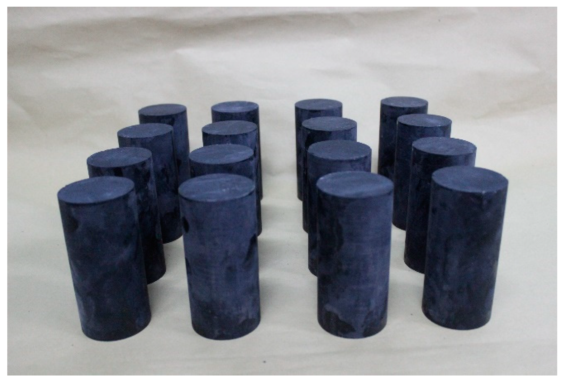
2.1. Triaxial Sample Preparation

The test samples were taken from the fresh outcrop black shale in Jiangkou, Wulong, Chongqing, in China, which is a natural extension of the southern marine shale gas reservoir in Fuling district. The samples were drilled in parallel with the bedding direction, and the cores were sealed and stored in a wax seal to prevent the contact from the air. Then the same rock block was drilled and processed into a standard sample of 50 × 100 mm, perpendicular to the bedding plane in the laboratory, to meet the requirements of the international rock mechanics test procedures [26]. As shown in Figure 1, the diameter tolerance was less than 0.2 mm, the unevenness of the end faces was less than 0.05 mm, and the vertical deviation of the end face from the axis was controlled within ±0.25°.

In order to further ensure the homogeneity of the rock samples and reduce the individual differences between them, the rock samples with initial cracks and initial damage were removed by visual observation. Additionally, the rock samples with significant differences in density and wave velocity, beyond 20% of the average value, were removed, and the effective screening of rock samples was realized to meet the accuracy requirements of rock mechanics tests.

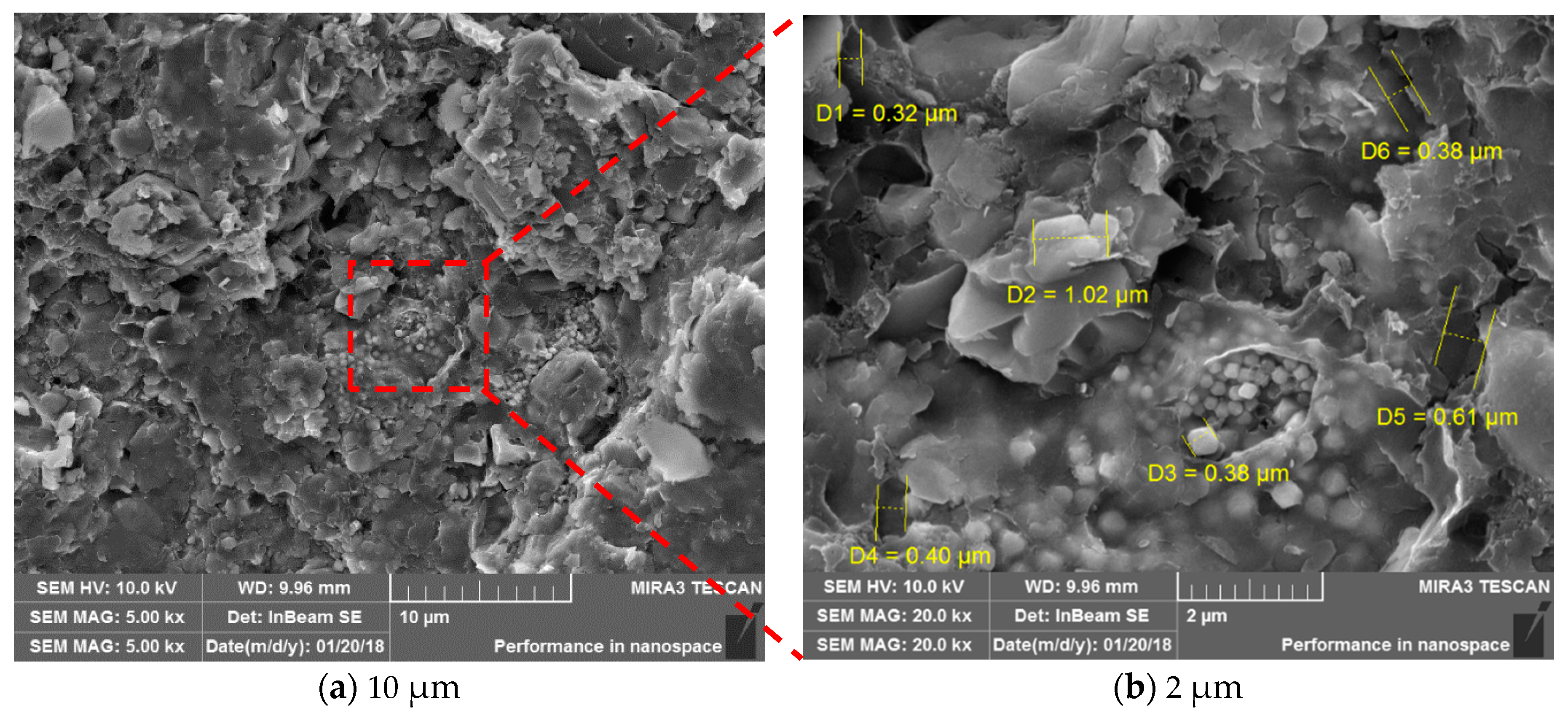
2.2. Basic Physical Properties of Shale

Before the shale triaxial unloading experiment, the basic physical properties of the shale were tested. Figure 2 shows the shale mineral diffraction pattern from the X-ray diffraction (XRD), and the primary minerals in the shale can be found as follows. The quartz was 55.9%, illite was 13.11%, albite was 13%, montmorillonite was 8.14%, calcite was 3.77%, pyrite was 3.74%, and dolomite was 2.34%.

The content of brittle minerals in the shale mineral composition is a significant factor determining the gas bearing, airtightness, and fracture ability of shale reservoirs. Generally, if the content of quartz and calcite in the shale is high, the brittleness pf the sample is stronger, and cracks are easily generated under the action of external force. In the process of geological evolution, natural unloading, such as uplifting and denudation, may cause shale gas leakage, which severely affects reservoir brittleness [27].

Figure 3 is a microscopic electron micrograph of the shale after magnifying 5000 times and 20,000 times, and the rock samples are characterized by pores of 10 and 2 μm, respectively. The pore size range was between 0.32 and 1.02 μm, and the shale gas was retained in the pores in the adsorption state, which was necessary to study the reservoir in depth and screen the exploration and development of favorable blocks. Therefore, it was of great significance to carry out indoor rock mechanics tests and to understand the mechanical properties of shale.

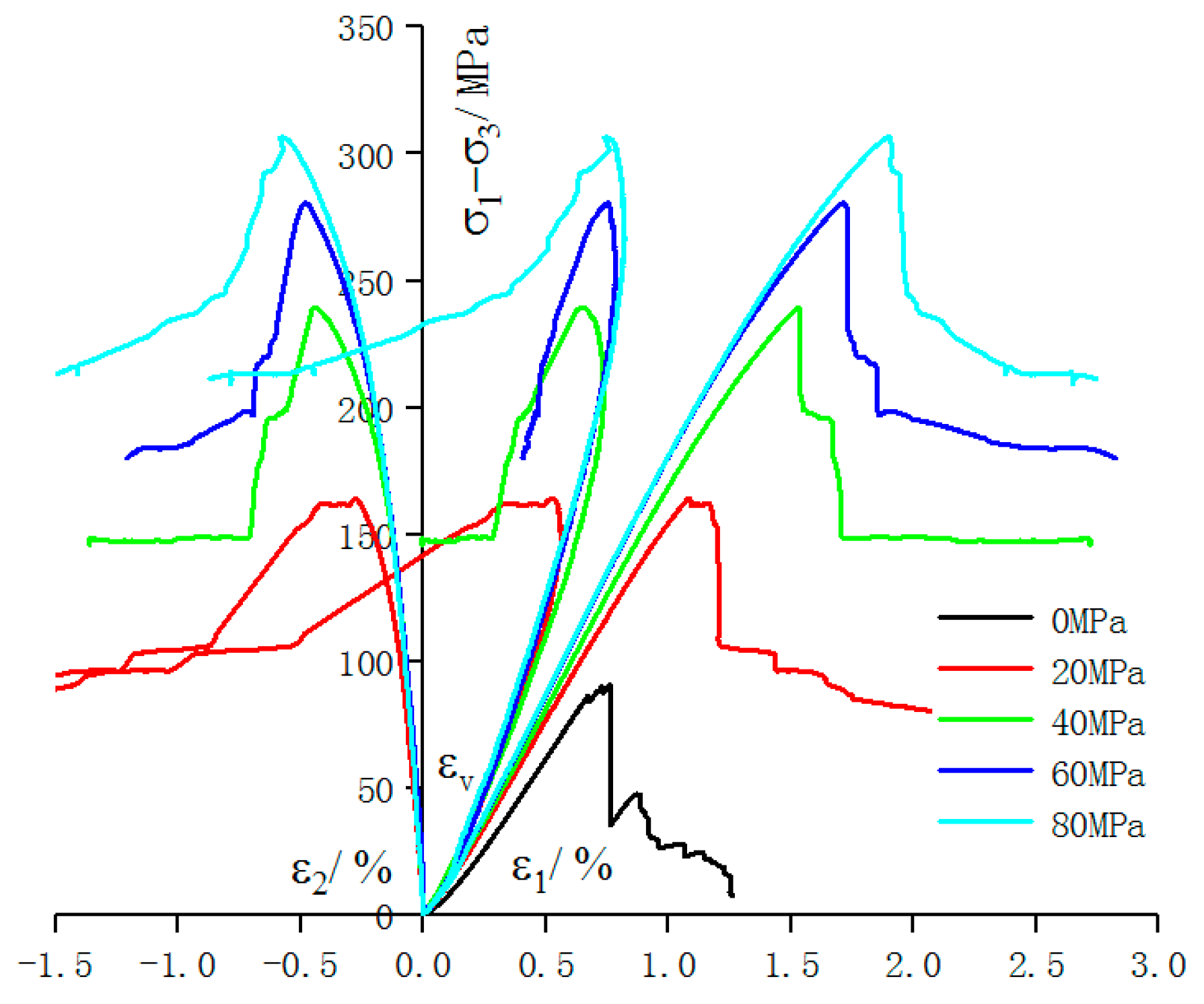
2.3. Conventional Triaxial Compression Test of Shale

Before designing the unloading triaxial compression experiment of shale, we needed to obtain the basic mechanical parameters of shale under conventional triaxial compression in advance to create the experimental unloading parameters. For this reason, the MTS (Mechanics Test System) 815.03 rock triaxial test system was adopted, and the principle of it is shown in Figure 4.

The testing machine comprises a loading part, a testing part, and a control part, whose control part includes a test assistant, a static test software, multifunctional test software, and a function generator control. It can achieve a fully automatic triaxial loading and measurement with full digital control. Based on this system, a conventional triaxial compression test with confining pressures of 0, 20, 40, 60, and 80 MPa was carried out, and the axial strain displacement control method was adopted with the loading rate of 0.001 mm/s.

Figure 5 is a triaxial stress–strain curve of the shale samples, ${\epsilon }_1$ represents axial strain, ${\epsilon }_2$ represents radial strain and ${\sigma }_1-{\sigma }_3$ represents axial pressure. It can be concluded from the curve that the peak strength and residual strength of the shale sample increase remarkably with the increase of confining pressure, and the elastic modulus and axial strain also increase gradually. The Mohr–Coulomb strength criterion is used to measure the peak strength and confining pressure from Figure 6.

$${\sigma }_1=k{\sigma }_3+b$$

(1)

After the curve is fitted, the following equation can be obtained. In Equation (1), $k$ and $b$ are the strength coefficients, which can be expressed by the internal friction angle and cohesion:

$$b=2c\cos \phi /(1-\sin \phi )$$

(2)

$$\begin{array}{c}k={\tan }^2(45°+\phi /2)\\ \phi ={35.36}^{°},c=27.34\mathrm{MPa}\end{array}$$

(3)

where the internal friction angle $\phi$ of the rock sample is 35.36°, and the cohesion $c$ is 27.34 MPa, indicating that the shale sample meets the Mohr–Coulomb strength criterion and has a good linear correlation with it. On this basis, the shale three-axis unloading test under different unloading rate conditions was carried out.

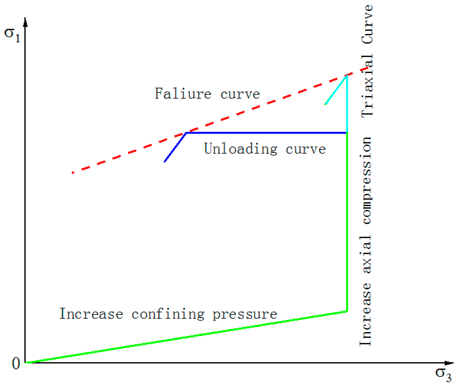
2.4. Unloading Test Plan

It can be seen in Figure 6 that under the confining pressure of 60 MPa, the shale sample has no obvious yielding characteristic when the deviatoric stress reaches 80% of the peak intensity, which is 280 MPa. Therefore, 60 MPa is selected as the unloading confining pressure [7], and the stress point at 80% of the peak strength is selected as the unloading point, that is, 224 MPa. The confining pressure was unloaded at a rate of 0.05, 0.1, 0.5, and 1.0 MPa/s, respectively, while maintaining the maximum principal stress the same until the sample was destroyed, reaching the peak of unloading, and then the experiment was stopped after the apparent stress step appeared. The changing of stress during unloading is shown in Figure 7. In particular, the part of the curve with the confining pressure in Figure 8 is a schematic diagram, highlighting the unloading curve. The slope of the real process should be 45°, and the maximum principal stress and the confining pressure increase in proportion.

3. Analysis of Test Results

3.1. Analysis of Unloading Experiment

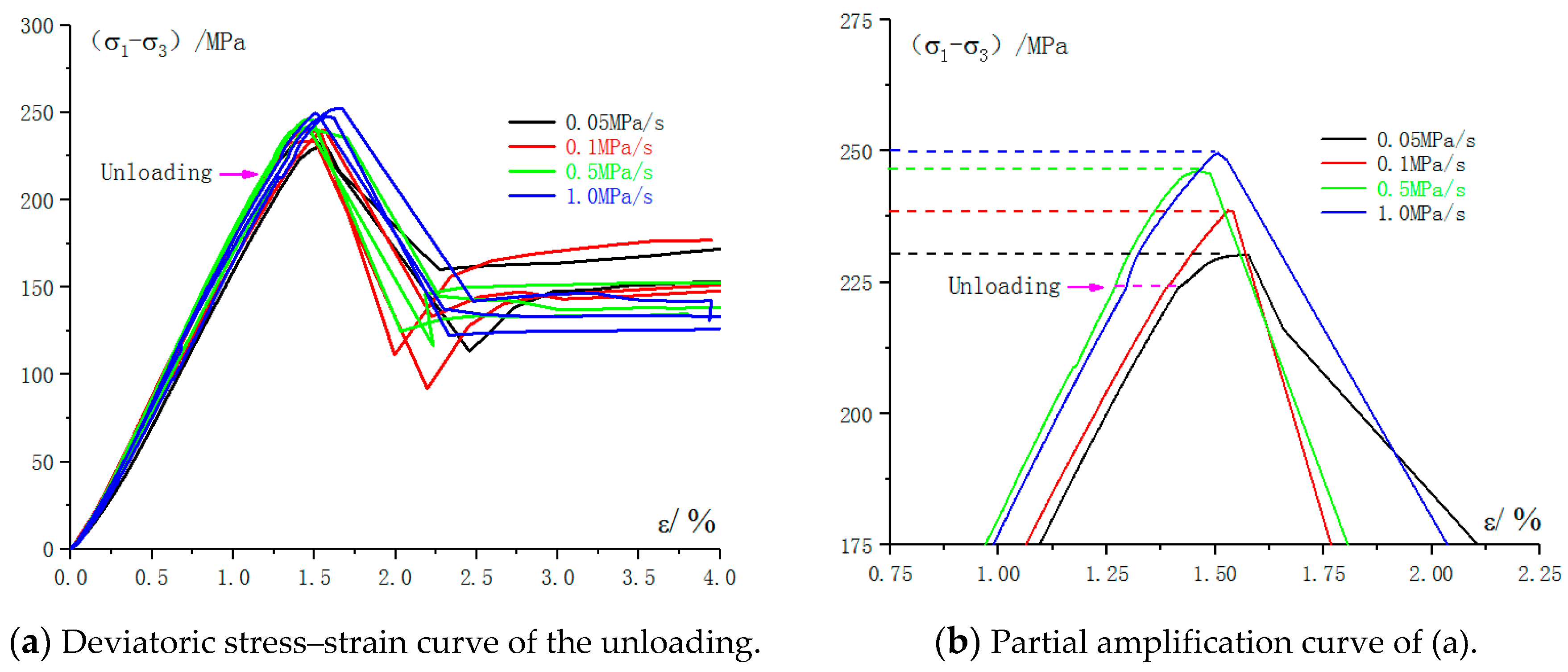
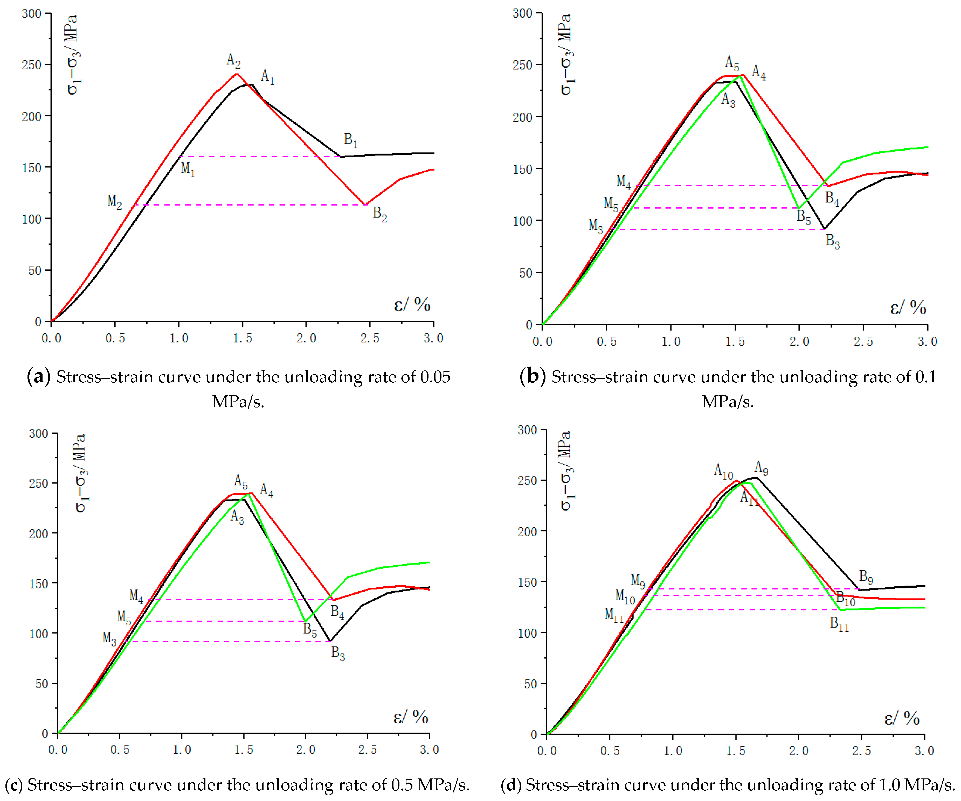
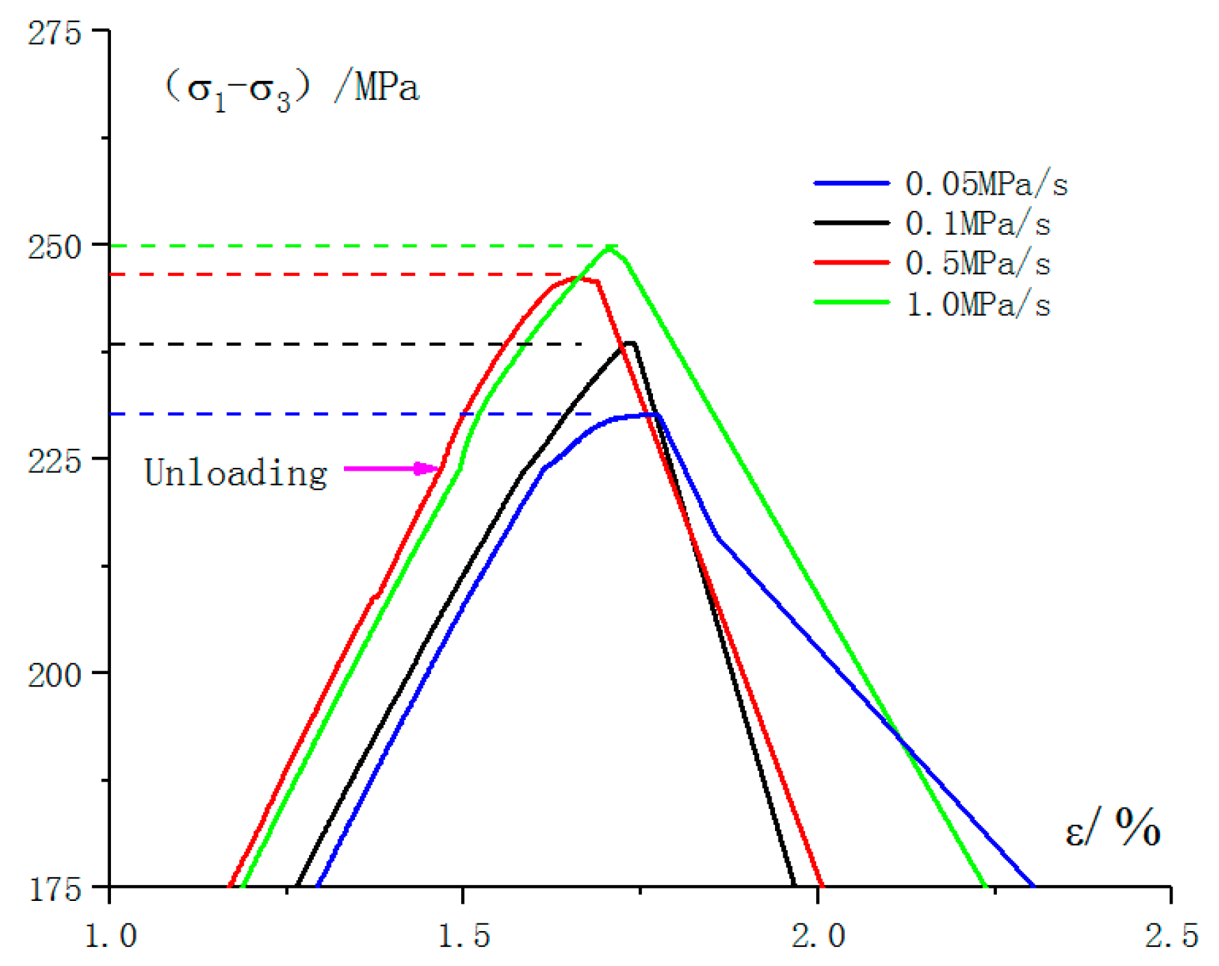
3.1.1. Stress–Strain Curve Analysis of Unloading

As shown in Figure 8, the different unloading rate deviatoric stress–strain curves of shale under 60 MPa confining pressure could be divided into compaction section, loading section, unloading section, peak section, and residual section. The compaction stage of shale was more apparent and shows that it had initial damage. Due to the continuous impact of high confining pressure and deviatoric stress, the shale produced noticeable elastic deformation, and the slope tended to be stable after the curve began to enter the loading section. Then at the unloading point, there was a significant unloading section, the curve showed a small amplitude deflection once again, and reached the peak section. It finally entered the residual section and stopped the test.

Before the unloading point, the stress–strain curves of the shale samples were in the elastic stage. After the unloading point, the stress–strain curve showed a significant deflection, deviated from the original straight-line segment, and entered into the next straight-line segment. The slope of the segment was smaller than the initial slope, that is, the deformation modulus of the rock sample decreased. As the deviatoric stress continued to increase, the curve deviated from the second straight line segment and entered the yielding stage. The axial strain also increased further and then came the peak section. The peak value of the shale stress was different under the condition of unloading rate, and the deformation and failure were more rapid than the conventional triaxial test. The deviatoric stress dropped sharply, and the stress slightly increased before the stress–strain curve reached the residual strength, especially at the unloading rate of and 0.5 MPa/s. Due to the increase of the unloading rate, the shale ruptured rapidly, and the confining pressure was too late to crush the broken shale, causing the deviatoric stress to drop too much. Then the broken shale was gradually pressed by the confining pressure, and the deviatoric stress slowly rose to reach the residual strength. Then, the deviatoric stress appeared to be the obvious stress step, the axial strain increased further, and the residual strength at different unloading rates showed a significant difference. The slope was relatively low at 0.05 MPa/s, relatively high at 1.0 MPa/s, and entered into the straight section again. The strength did not change significantly until the end of the test; at last, the test system was stopped.

As shown in

Table 1. Experimental plan and related parameters.

Serial Number	Density g/cm3	ε1	ε2	ε3	σ3 (MPa)	$\mathit{v}*(\mathbf{MPa}/\mathbf{s})$	$\mathbf{lg}(\mathbf{v}*)$	${({\mathit{\sigma }}_1-{\mathit{\sigma }}_3)}_{\mathbf{max}}^{*}\left(\mathbf{MPa}\right)$	$\mathbf{l}\mathbf{g}({({\mathit{\sigma }}_1-{\mathit{\sigma }}_3)}_{\mathbf{max}}^{*})$	${({\mathit{\sigma }}_1-{\mathit{\sigma }}_3)}^{*}\left(\mathbf{MPa}\right)$	$\mathbf{lg}({({\mathit{\sigma }}_1-{\mathit{\sigma }}_3)}^{*})$	${\mathit{\sigma }}_3^{*}\left(\mathbf{MPa}\right)$	$\mathbf{lg}({\mathit{\sigma }}_3^{*})$
RF-1-15	2.54	1.78	0.22	1.33	60	0.05	−1.3	229.73	2.36	165.86	2.22	54.27	1.74
RF-4-11	2.51	1.70	0.27	1.16	60	0.05	−1.3	239.61	2.38	151.70	2.18	44.39	1.65
RF-2-6	2.52	1.68	0.30	1.07	60	0.1	−1	233.42	2.39	148.08	2.17	50.79	1.71
RF-3-3	2.52	1.86	0.38	1.11	60	0.1	−1	239.82	2.38	145.49	2.16	44.92	1.65
RF-4-2	2.52	1.74	0.27	1.19	60	0.1	−1	238.48	2.38	174.39	2.24	46.11	1.66
RF-2-5	2.52	1.64	0.36	0.92	60	0.5	−0.3	241.51	2.38	137.32	2.14	43.09	1.63
RF-3-4	2.53	1.62	0.40	0.81	60	0.5	−0.3	240.82	2.38	151.60	2.18	43.57	1.64
RF-3-5	2.53	1.69	0.34	1.02	60	0.5	−0.3	246.22	2.39	132.95	2.12	38.64	1.59
RF-2-2	2.52	1.95	0.45	1.05	60	1.0	0	252.00	2.40	142.00	2.15	32.76	1.52
RF-2-9	2.52	1.73	0.28	1.17	60	1.0	0	249.63	2.40	132.95	2.12	35.11	1.55
RF-4-5	2.53	1.83	0.51	0.82	60	1.0	0	247.88	2.40	125.00	2.10	36.69	1.57

, the unloading rate had a significant effect on the axial strain, radial strain, and peak stress. For axial strain ${\epsilon }_1$, as the unloading rate increased, the average, from small to large, rate was 1.7335, 1.7529, 1.648, and 1.837. Although there was a fluctuation, the overall increasing trend was still obvious. When the unloading rate $v^{*}$ was 1.0 MPa/s, the average value of axial strain reached 1.837%, which was 6.0% higher than 0.05 MPa/s, and the peak value increased by 1.952%. In terms of radial strain, there was a significant increase with the increase in rate. The average value at different rates was 0.2459, 0.316, 0.3662, and 0.4212. The shale tended to rapidly increase in the radial strain under high rate, with an increase of 71.2% compared to 0.05 MPa/s, which was a huge change compared to the increase of 6.0% in axial strain. That is, under unloading conditions, the radial strain increased much more than the axial strain. In terms of volumetric strain, it was 1.246, 1.1253, 0.9157, and 1.102. The volumetric strain showed a decreasing trend with the increase of the unloading rate, which was gradually weakened by the expansion effect.

In the Table 1, $v*$ represents the unloading rate, MPa/s; $\lg (v^{*})$ represents the logarithm of unloading rate; ${({\sigma }_1-{\sigma }_3)}_{\max }$ represents the maximum axial pressure, MPa; $\lg ({({\sigma }_1-{\sigma }_3)}_{\max })$ represents the logarithm of maximum axial pressure; ${({\sigma }_1-{\sigma }_3)}^{*}$ represents the residual stress, MPa; $\lg ({({\sigma }_1-{\sigma }_3)}^{*})$ represents the logarithm of residual stress; ${\sigma }_3^{*}$ represents the failure confining pressure, MPa; $\lg {\sigma }_3^{*}$ represents the logarithm of failure confining pressure.

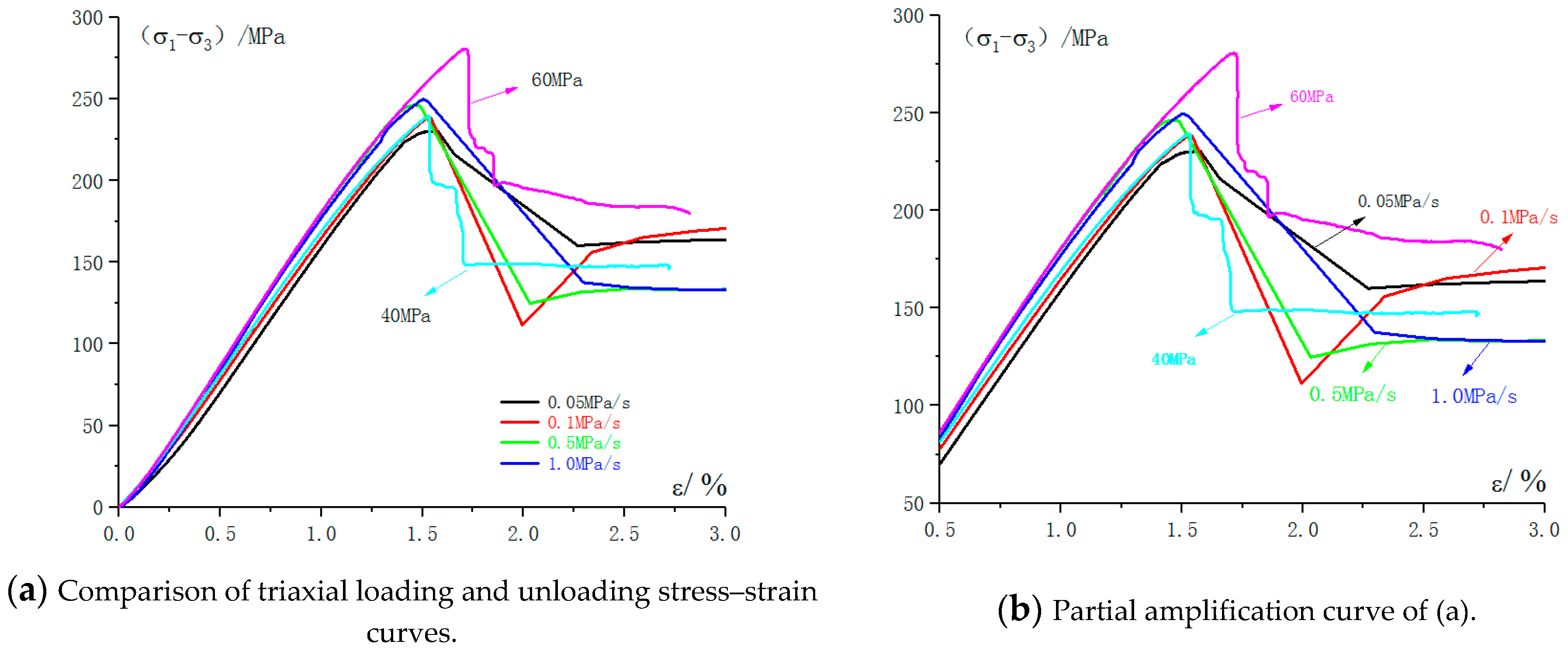
3.1.2. Comparative Study on the Stress–Strain Curves of Loading and Unloading

The deviatoric stress–strain curves of the 40 and 60 MPa confining pressures in the full-process stress–strain curve of Figure 5 of shale are extracted, and the typical deviatoric stress–strain curves at four unloading rates are selected, which is shown in Figure 9.

The unloading stress–strain curve of the 60 MPa confining pressure in Figure 9 shows that it is between the 40 MPa confining pressure and the 60 MPa confining pressure of the triaxial loading test. The stress–strain curve under loading and unloading are entirely different after the peak point. During the triaxial loading test, the peak intensity is higher, and the curve drop rate is faster, the partial stress falls by a large piece when the axial stress changes are tiny. Under the unloading conditions, the peak strength of shale is reduced significantly. At the unloading rate of 0.05 and 0.1 MPa/s, the peak intensity is very close to the peak intensity of 40 MPa loading curve. At the unloading rate of 0.5 and 1.0 MPa/s, the peak intensity is slightly higher than the peak intensity of the 40 MPa loading and less than the peak intensity of the 60 MPa loading. At the same time, the residual strength of the unloading is also reduced. At the unloading rate of 0.05 and 0.1 MPa/s, the residual strength is about 160 MPa, which is higher than the residual strength of 40 MPa loading curve and less than the 60 MPa loading curve. While the unloading rate is 0.5 and 1.0 MPa/s, the residual strength is only about 140 MPa, which is lower than the residual strength under 40 MPa confining pressure, and the curve drop rate is also weakened. That is to say, compared with the loading curve, the unloading has a noticeable weakening effect on the peak strength and residual strength of shale samples. At the same time, there is an excellent relationship between the weakening mechanical parameters and the unloading rate.

3.2. Influence of Unloading Rate on Shale Mechanical Parameters

The peak strength ${({\sigma }_1-{\sigma }_3)}_{\max }$ and residual stress ${({\sigma }_1-{\sigma }_3)}^{*}$ are essential parameters in hydraulic fracturing mining. They are important indicators that cannot be ignored in regional airtightness evaluation. As shown in Table 1, the critical analysis of this paper is as follows.

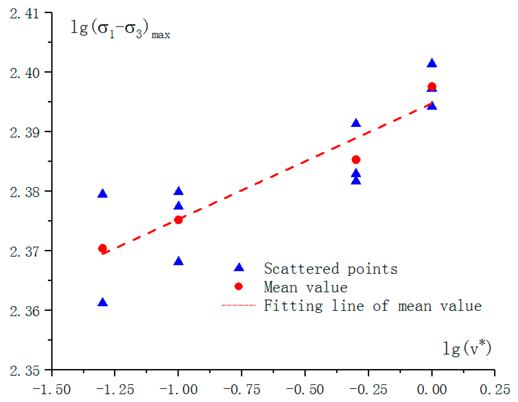
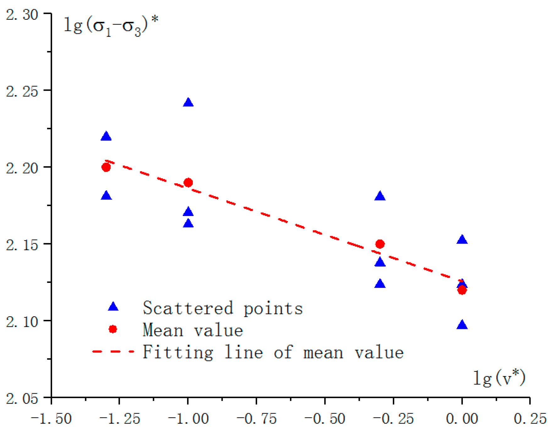
3.2.1. Effect of Unloading Rate on Peak Intensity

Figure 10 is a graph of peak intensity versus unloading rate. Although the peak intensity is discrete, the total increases with the increase of the unloading rate. Under the condition of high unloading rate, the deformation of the shale lags behind the stress, and the partial deformation is too late when the stress reaches a significant value. Thus, the shale exhibits a higher unloading bias stress. In Figure 10, $\log ({\mathrm{v}}^{*})$ and $\lg {({\sigma }_1-{\sigma }_3)}_{\max }$ has a significant linear relationship, and are fitted as follows.

$$\lg {({\sigma }_1-{\sigma }_3)}_{\max }=0.019\lg ({\mathrm{v}}^{*})+2.395,R^2=0.95$$

(4)

$${({\sigma }_1-{\sigma }_3)}_{\max }={({\mathrm{v}}^{*})}^{0.019}+248.31$$

(5)

The fitting curve shows that $\lg {({\sigma }_1-{\sigma }_3)}_{\max }$ and $\log ({\mathrm{v}}^{*})$ has a significant linear correlation, and the mean is better distributed on the upper and lower sides of the curve. The southern marine shale experienced multiple periods of uplift and erosion, and the shale reservoir gradually discharged once and again. The faster the reservoir is lifted, the higher the deviatoric stress of the internal accumulation, which may be more detrimental to the next exploration and development.

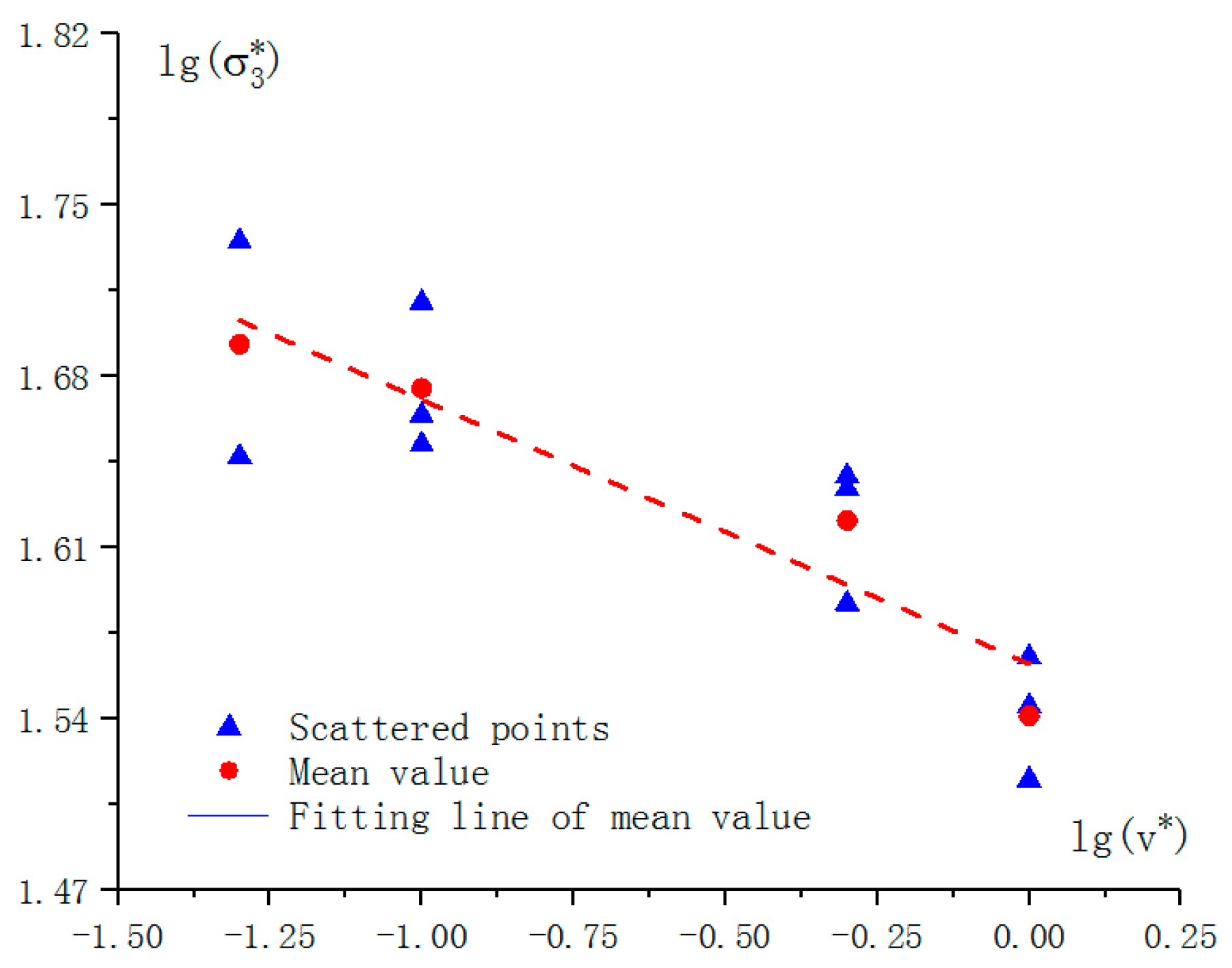
3.2.2. Influence of Unloading Rate on Destructive Confining Pressure

With the increase of the unloading rate $v^{*}$, the destructive confining pressure ${\sigma }_3^{*}$ decreases obviously, which is shown in Figure 11. In the geological process, the destructive confining pressure usually corresponds to the overlying stress, which means the overlying stress is becoming smaller and smaller. These parameters are fitted as follows.

$$\lg ({\sigma }_3^{*})=-0.108\lg ({\mathrm{v}}^{*})+1.562,R^2=0.91$$

(6)

$${\sigma }_3^{*}={(v^{*})}^{-0.108}+36.475$$

(7)

It can be concluded from the fitting curve that ${\sigma }_3^{*}$ and $v^{*}$ have a significant linear negative correlation, and the mean is also better distributed on the upper and lower sides of the curve. As the unloading rate increases, the performance of the confining pressure is gradually reduced.

3.2.3. Effect of Unloading Rate on Residual Stress

Using the data processing method of 3.2.1, as shown in Figure 12, the residual stress $({\sigma }_1-{\sigma }_3{)}^{*}$ and the unloading rate $v^{*}$ are closely related. With the increase of $v^{*}$, the residual strength gradually decreases, indicating that $v^{*}$ has a weakening effect to the shale, although the data has a discrete type, the mean has a distinct linear relationship and fits it as follows.

$$\lg {({\sigma }_1-{\sigma }_3)}^{*}=-0.061\lg ({\mathrm{v}}^{*})+2.126,R^2=0.974$$

(8)

$${({\sigma }_1-{\sigma }_3)}^{*}={(v^{*})}^{-0.0611}+164.48$$

(9)

Figure 12 shows that with the increase of unloading rate, the mechanical parameters of shale significantly changed, and the residual stress decreased dramatically. The residual stress can reflect the residual strength of the shale reservoir after the geological movement and the hydraulic fracturing during the development process. It is of great significance for the settlement of the site, the deformation of the ground, and the study of the disaster mechanism of shale gas exploration and development.

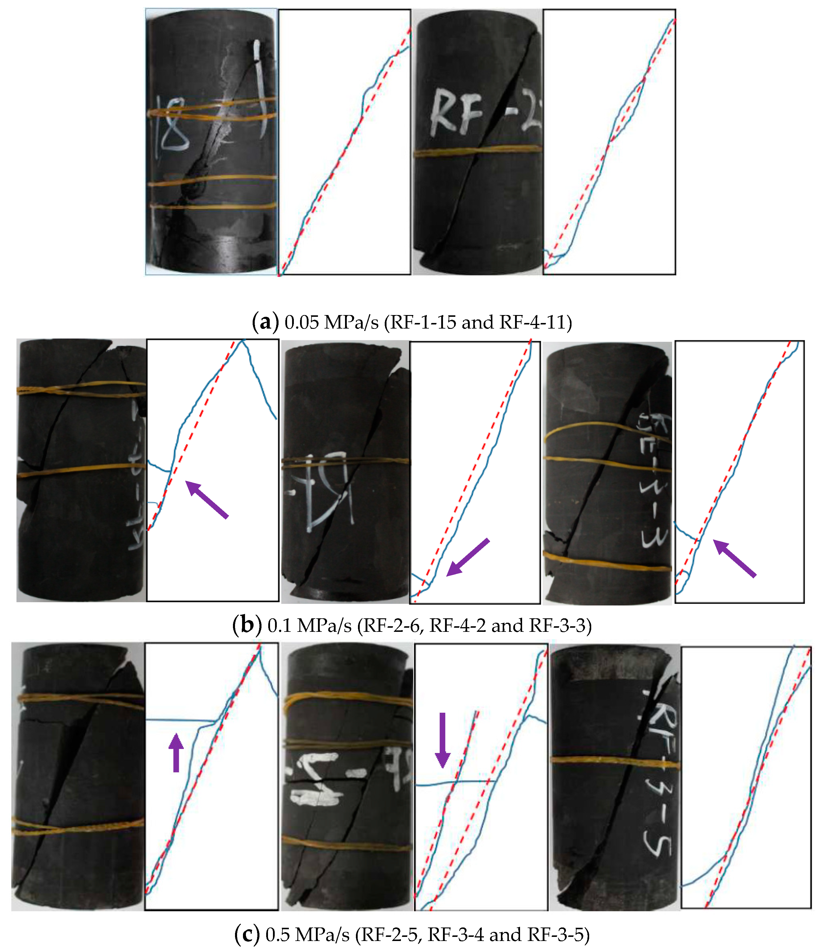
3.3. Influence of Unloading Rate on Shale Failure Characteristics

In Figure 13, it shows that the failure modes of the shale triaxial unloading test at different unloading rates, corresponding to the samples in Table 1, which can be concluded that the shale failure pattern and the unloading rate $v^{*}$ have a great relationship.

When $v^{*}$ is 0.05 MPa/s, the failure mode of the rock is milder and the damage is more uniform. Based on a typical single bevel shear failure, the shear surface runs through the entire shale, which has visible friction marks.

When $v^{*}$ is 0.1 MPa/s, the shale fracture morphology began to become complicated. In addition to the oblique section shear failure, fine cracking begins to occur, concentrated on the edge of the shear band. As shown by the arrows in Figure 13b, several tiny cracks perpendicular to the shear band appear and penetrate the entire cleaved surface to form a macroscopic network of cracks. According to the analysis, due to the increase of the unloading rate, the weak structural surface inside the shale sample is opened in the vertical direction under the action of shearing force, forming a small part of local cracking.

When $v^{*}$ is 0.5 MPa/s, the rupture characteristics tend to be apparent, and the central shear zone still runs through the entire shale sample. At the same time, at the height of one third and one half of the sample, 0°, that is, the crack of the bedding plane occurs. With the further increase of the unloading rate, the bedding plane is also cracked due to the local tension stress resulted from the accelerated rate. There are secondary lateral distribution cracks between the fracture surfaces, and the shale fracture grid tends to be complicated. In the RF-2-5 sample, the sample at the intermediate position, a secondary shear band appears. Although a macroscopic crack is formed, the through slit is not formed.

When $v^{*}$ is 1.0 MPa/s, with the primary shear zone, the frequency of the secondary non-penetrating shear band increases, and as the unloading rate increases gradually, the weak layer and the structural plane continue to crack, showing the simultaneous shearing of the three shear bands. There are secondary shear bands parallel to the main shear zone, horizontal cracks parallel to the bedding seam, and cracks perpendicular to the primary shear zone. These cracks cause the instability and destruction of the shale as a whole and eventually form a complex fracture network, which quickly leads to the leakage of shale gas during geological changes and affects its exploration and development.

4. Discussion of Rock Brittleness

4.1. Evaluation of Rock Brittleness

The brittleness of shale can significantly affect the stability of the borehole wall and the fracturing effect during on-site development. It is a crucial indicator for evaluating the mechanical properties of the reservoir and is an essential basis for selecting the perforation reconstruction layer and designing the fracturing technology [28]. The establishment of brittleness indicators will help to analyze the brittleness of shale further.

At present, scholars at home and abroad have proposed a variety of methods based on energy, hardness, mineral composition, logging curve, expansion inflection point, pump pressure curve, debris content, fracture toughness, tensile strength ratio, full stress–strain curve, etc. The brittleness evaluation methods are summarized in

Table 2. Research table of brittleness evaluation methods from domestic and foreign scholars.

Method	Equation	Description	Resource
Pressing ratio	$B_1={\sigma }_c{\sigma }_t/2$	Mean of the product of uniaxial compressive strength ${\sigma }_c$ and tensile strength ${\sigma }_t$.	Altindag [29]
Pressing ratio	$B_2={({\sigma }_c{\sigma }_t/2)}^{1/2}$	The function of uniaxial compression ${\sigma }_c$ and tensile strength ${\sigma }_t$ ratio.	Altindag [29]
Pressing ratio	$B_3={\sigma }_c/{\sigma }_t$	The ratio of uniaxial compressive strength ${\sigma }_c$ to tensile strength ${\sigma }_t$.	Hucka and Das [30]
Pressing ratio	$B_4=({\sigma }_c-{\sigma }_t)/({\sigma }_c+{\sigma }_t)$	The function of uniaxial compression and tensile strength ratio.	Hucka and Das [30]
Hardness test	$B_5=(H_m-H)/K$	$H$ is the macro hardness and $H_m$ is the micro hardness.	Honda and Sanada [31]
Hardness, fracture test	$B_6=HE/K_{IC}{}^2$	$H$ is a hardness coefficient, $E$ is Young’s modulus, and $K_{IC}$ is the fracture toughness.	J. B. Quinn and G. D. Quinn [32]
Hardness, fracture test	$B_7=H/K_{IC}$	$H$ is a hardness coefficient, $E$ is Young’s modulus, and $K_{IC}$ is the fracture toughness.	Lawn and Marshall [33]
Hardness test	$B_8=K_{IC}/({\sigma }_y{h}^{1/2})$	$K_{IC}$ is the fracture toughness, ${\sigma }_y$ is the yield stress, and $h$ is the characteristic size of the sample.	Bazant and Kazemi [34]
Bazant curve	$B_9=E{G}_F/{\sigma }_t{}^2$	The ratio of elastic energy to fracture energy, $G_F$ is the fracture energy, $E$ is elastic modulus, and ${\sigma }_t$ is Hllebrgorg characteristic length value.	Bazant and Kazemi [34]
Cohesion-weakening-friction-strengthening (CWFS) model	$B_{10}=({\epsilon }_f{}^p-{\epsilon }_c{}^p)/{\epsilon }_c{}^p$	${\epsilon }_f^p$ and ${\epsilon }_c^p$ is the plastic strain when the friction strength and cohesive force reaches the final limit value, respectively.	Hajiabdolmajid et al. [35]
Penetration test	$B_{11}=P_{dec}/P_{inc}$	The ratio of incremental load to decay load.	Copur [36]
Penetration test	$B_{12}=F_{\max }/P$	The ratio of the maximum impact load to the penetration depth.	Yagiz [37]
Impact test	$B_{13}=S_{20}$	Percentage of fine debris less than 11.2 mm in diameter.	Blindheim and Bruland [38]
Impact test	$B_{14}=q{\sigma }_c$	$q$ is the percentage that less than 0.6 mm of debris and ${\sigma }_c$ is uniaxial compressive strength.	Protodyakonov [39]
Mohr stress circle	$B_{15}=\sin \phi$	Sinusoidal value of internal friction angle.	Hucka and Das [30]
Mohr stress circle	$B_{16}={45}^{\circ }+\phi /2$	The function of the internal friction angle.	Hucka and Das [30]
Mineral composition analysis	$B_{17}=(W_{qtz}+W_{carb})/W_{total}$	The ratio of brittle mineral content to total mineral content.	Rickman et al. [40]
Mineral composition analysis	$B_{18}=\frac{w_{qtz}}{w_{total}}\times 100\%$	The ratio of quartz to total mineral content.	Jarvie [41]
Energy dissipation, stress–strain curve	$B_{19}=\frac{d{W}_r}{d{W}_e}$	The ratio of rupture energy per unit volume consumption to elastic energy released internally.	Heng et al. [42]
Stress–strain curve	$\begin{array}{l}{B}_{20}=({\epsilon }_{BRIT}-{\epsilon }_n)/({\epsilon }_m-{\epsilon }_n)\\ +\alpha C{S}_{BRIT}+\beta C{S}_{BRIT}+\eta \end{array}$	The sum of the peak strain index and the post-peak curve shape index.	Li et al. [43]
Stress–strain curve	$B_{21}=W_r/W$	The ratio of recoverable strain energy to total energy.	Hucka and Das [30]
Stress–strain curve	$B_{22}=A_2/A_1$	$A_1$ is the area under the oblique line of the peak intensity point with the deformation modulus as the slope and $A_2$ is the area under the loading curve.	Aubertin et al. [44]
Stress–strain curve	$B_{23}=\alpha {\sigma }_c{\epsilon }_f/({\sigma }_t{\epsilon }_b)$	${\sigma }_c$ is uniaxial compressive strength, ${\sigma }_t$ is tensile strength, ${\epsilon }_f$ and ${\epsilon }_b$ is a pre-peak and a post-peak strain, respectively, and $\alpha$ is adjustment parameter.	Feng et al. [45]
Stress–strain curve	$B_{24}={\epsilon }_{1i}$	${\epsilon }_{1i}$ is an unrecoverable axial strain when the specimen is broken, it is brittle when ${\epsilon }_{1i}$ < 3%, brittle plasticity when ${\epsilon }_{1i}$ at 3%–5%, and plasticity when ${\epsilon }_{1i}$ > 5%.	George [46]
Stress–strain curve	$B_{25}=\overline{E}+\overline{\nu }$	The ratio of normalization of elastic modulus and Poisson.	Rickman et al. [40]
Stress–strain curve	$B_{26}={\epsilon }_r/\epsilon$	The ratio of recoverable strain ${\epsilon }_r$ to total strain $\epsilon$.	Hucka and Das [30]
Stress–strain curve, Fracture test	$B_{27}=L{\sigma }_t{}^2/E{G}_F$	The ratio of elastic energy to fracture energy, $G_F$ is the fracture energy, $E$ is elastic modulus, and ${\sigma }_t$ is characteristic length value.	Bazant and Kazem [34]
Stress–strain curve	$B_{28}=({\tau }_p-{\tau }_r)/{\tau }_p$	${\tau }_p$ is the peak strength and ${\tau }_r$ is the residual strength.	Bishop [47]
Stress–strain curve	$B_{29}=({\epsilon }_p-{\epsilon }_r)/{\epsilon }_p$	The function of is peak strain ${\epsilon }_p$ and residual strain ${\epsilon }_r$.	Ajiabdolmajid and Kaiser [35]
Stress–strain curve	$B_{30}=d{W}_r/d{W}_e=(E-M)/M$	The ratio of fracture damage energy to pre-peak elastic strain energy after rock rupture peak.	Stavrogin and Tarasov [48]
Stress–strain curve	$B_{31}=\frac{{\tau }_p-{\tau }_r}{{\tau }_p}\frac{\lg \left|k_{ac(\mathrm{AC})}\right|}{10}$	${\tau }_p$ is the peak strength, ${\tau }_r$ is the residual strength, and $k_{ac(\mathrm{AC})}$ is the slope of different peak intensity points to the drop point, respectively.	Zhou et al. [49]
Stress–strain curve	$\begin{array}{l}{B}_{32}=\alpha \exp \left[\frac{{\epsilon }_B-{\epsilon }_A}{({\sigma }_r+{\sigma }_3-2\mu {\sigma }_3)/\mathrm{E}-{\epsilon }_A}\right]\\ +\beta (1-{\sigma }_r/{\sigma }_a)+\gamma \left[1-\exp (\mathrm{M}/\mathrm{E})\right]\end{array}$	${\sigma }_a$ is the peak strength, ${\sigma }_r$ is the residual strength, ${\epsilon }_A$, ${\epsilon }_B$, and ${\epsilon }_M$ are the axial strain and $\alpha +\beta +\gamma =1$.	Hou et al. [27]
Stress–strain curve	$\begin{array}{l}{B}_{33}=\exp \left[\frac{{\epsilon }_B-{\epsilon }_A}{({\sigma }_r+{\sigma }_3-2\mu {\sigma }_3)/\mathrm{E}-{\epsilon }_A}\right]\\ \times (1-{\sigma }_r/{\sigma }_a)\times \left[1-\exp (\mathrm{M}/\mathrm{E})\right]\end{array}$	${\sigma }_a$ is the peak strength, ${\sigma }_r$ is the residual strength, and ${\epsilon }_A$, ${\epsilon }_B$, and ${\epsilon }_M$ is the axial strain.	Hou et al. [27]

as a total of 33 kinds. Most of their research results are based on their respective research purposes and are used in their respective fields. Based on the stress–strain curve, this paper comprehensively compares several brittleness evaluation methods and attempts to explore their application under unloading conditions.

Hou et al. [27] combine brittleness and stress drop coefficient $P$, softening modulus $M$, and brittle drop coefficient $R$:

$$R=-({\epsilon }_B-{\epsilon }_A)/({\epsilon }_M-{\epsilon }_A)$$

(10)

$$M=({\sigma }_a-{\sigma }_r)/({\epsilon }_A-{\epsilon }_B)$$

(11)

$$P=({\sigma }_a-{\sigma }_r)/{\sigma }_a$$

(12)

where ${\sigma }_a$ represents the peak intensity of the sample at point A, ${\sigma }_r$ represents the residual strength of the sample at point B, and ${\epsilon }_A$, ${\epsilon }_B$, ${\epsilon }_M$ represent the axial strain of the sample at points A, B, and M, respectively in Figure 14.

Then the brittleness index $B_1$, $B_2$, $B_3$ are defined, and the normalization is done:

$$B_1=exp(-R)$$

(13)

$$B_2=({\sigma }_{\mathrm{a}}-{\sigma }_r)/{\sigma }_{\mathrm{a}}$$

(14)

$$B_3=1-exp(M/E)$$

(15)

Comprehensive evaluation coefficient $B_{d1}$ and $B_{d2}$ are proposed (i.e., in

Table 3. Table of detailed parameters of shale sample brittleness.

	Confining Pressure	0	20	40	60	80
Parameters
${\epsilon }_B$		0.76	1.21	1.71	1.86	2.37
${\epsilon }_A$		0.76	1.16	1.53	1.72	1.91
$E$		11.10	16.09	17.38	18.82	18.83
${\sigma }_r$		35.58	106.18	149.83	196.79	216.49
${\sigma }_3$		0.00	20.00	40.00	60.00	80.00
$\mu$		0.24	0.18	0.17	0.21	0.23
${\sigma }_A$		90.58	162.42	239.33	280.45	306.60
$M$		−1375.00	−117.17	−52.34	−60.63	−19.34
$B_1$		1.00	1.01	1.02	1.01	1.04
$B_2$		0.61	0.35	0.37	0.30	0.29
$B_3$		1.00	1.00	0.95	0.96	0.64
$B_{d1}$		0.87	0.78	0.78	0.76	0.66
$B_{d2}$		0.61	0.35	0.36	0.29	0.20

):

$$B_{d1}=\alpha B_1+\beta B_2+\gamma B_3$$

(16)

$$B_{d2}=B_1\times B_2\times B_3$$

(17)

where $\alpha +\beta +\gamma =1$, $\alpha$, $\beta$, $\gamma$ represents the weights in the total brittleness index $B_1$, $B_2$, $B_3$, respectively, and can be valued according to the same standard, or may be based on the focus of the project and the different purposes of the research.

Combined with the triaxial stress–strain curve of the samples in Figure 5, and when $\alpha =\beta =\gamma =1/3$ is selected, then the following table can be developed.

It can be seen that the brittleness of the shale sample is well characterized by the brittleness index $B_{d1}$ and $B_{d2}$, and they decrease continuously with the increase of confining pressure, which plays a proper role in the characterization with the failure of samples in the 3.3-page. Additionally, compared with $B_{d1}$, the numerical range of $B_{d2}$ is more extensive, and the high brittleness characteristics of shale samples under uniaxial compression can be highlighted, which proves the useful application of the method in triaxial loading test.

4.2. Evaluation of Brittleness during Unloading

4.2.1. Existing Brittleness Evaluation Method

It is equally important to evaluate the brittleness under unloading conditions. The method of the same literature [28] is used to select the peak intensity point $A_1$ to $A_{11}$, the residual unloading rate $B_1$ to $B_{11}$, the residual intensity point, and the intersection with the elastic section $M_1$ to $M_{11}$, which is shown in Figure 15:

After a large number of parameter calculations,

Table 4. Evaluation form of shale unloading brittleness index.

	No.	1	2	3	4	5	6	7	8	9	10	11
Parameters
${\sigma }_A$		230.26	240.44	233.42	239.82	238.61	241.51	240.82	246.22	252.00	249.63	247.88
${\sigma }_B$		160.10	113.15	91.95	133.20	111.36	144.95	116.54	120.80	142.00	137.48	122.59
${\sigma }_M$		160.10	113.15	91.95	133.20	111.36	144.95	116.54	120.80	142.00	137.48	122.59
${\epsilon }_A$		1.57	1.45	1.51	1.54	1.57	1.45	1.47	1.46	1.67	1.51	1.57
${\epsilon }_B$		2.27	2.46	2.19	2.22	1.99	2.27	2.23	2.03	2.48	2.30	2.33
${\epsilon }_C$		1.01	0.65	0.55	0.74	0.69	0.79	0.71	0.71	0.81	0.77	0.77
$E$		17.81	17.74	18.44	18.28	16.69	18.52	17.56	18.07	17.35	18.16	17.03
$u$		0.21	0.27	0.29	0.26	0.27	0.32	0.26	0.25	0.24	0.23	0.25
$M$		−10.02	−12.60	−20.80	−15.68	−30.30	−11.78	−16.35	−22.00	−13.58	−14.20	−16.49
$B_1$		1.00	1.00	1.00	1.00	1.00	1.00	1.00	1.00	1.00	1.00	1.00
$B_2$		0.30	0.53	0.61	0.44	0.53	0.40	0.52	0.51	0.44	0.45	0.51
$B_3$		0.43	0.51	0.68	0.58	0.84	0.47	0.61	0.70	0.54	0.54	0.62
$B_{d1}$		0.58	0.68	0.76	0.67	0.79	0.62	0.71	0.74	0.66	0.66	0.71
$B_{d2}$		0.13	0.27	0.41	0.26	0.45	0.19	0.31	0.36	0.24	0.24	0.31

can be obtained. The first row 1–11 of the table corresponds to the 11 unloading curves in Figure 16, and each curve is divided into three points: M, A, and B. Where point A is the peak point of the stress–strain curve, representing the maximum intensity of the pattern at the time of unloading; point B is the brittle drop point, representing the residual intensity after the peak; and point M is the intersection of the parallel line of the point B and the elastic section. Furthermore, ${\sigma }_A$, ${\sigma }_B$, ${\sigma }_M$, respectively correspond to the stress values of points A, B, and M in Figure 16, whose unit is MPa. ${\epsilon }_A$, ${\epsilon }_B$, ${\epsilon }_M$ represents the axial strain values of three points: A, B, and M, respectively, whose unit is %. $E$ is the elastic modulus, whose unit is Gpa. $\mu$ is the Poisson’s ratio, dimensionless. $M$ is softening modulus, dimensionless. $B_1$, $B_2$, $B_3$ are different brittleness indicators, dimensionless. $B_d$ is the comprehensive evaluation coefficient, dimensionless.

At four unloading rates, the elastic modulus is relatively close, fluctuating between 16.69 and 18.52, and the average values are 17.78, 17.80, 18.05, and 17.51 GPa, respectively. Poisson’s ratio is also relatively close, fluctuating between 0.21 and 0.32, the average values are 0.24, 0.27, 0.28, and 0.24, respectively.

According to the above table, the brittleness index $B_{d1}$ shows a trend of increasing first and then decreasing. The average values at the four unloading rates are 0.63, 0.74, 0.69, and 0.68, respectively, and the brittleness fluctuates significantly under the same unloading rate, such as the unloading rate 0.05 MPa/s, it is 0.58 and 0.68, respectively. The obtained discrete type of $B_{d1}$ is higher, which is inconsistent with the brittleness of the fractured specimen. The brittleness index $B_{d2}$ also shows a trend of increasing first and then decreasing. The average values at the four unloading rates are respectively 0.24, 0.27, 0.28, and 0.24, the gap is small, and the brittleness of shale samples under unloading conditions cannot be characterized. According to the analysis of this paper, the stress path segment from the unloading point to the deviatoric stress is ignored during the calculation, as shown in Figure 16.

Combined with Figure 10, it can be concluded that the unloading stress–strain curve of the 60 MPa confining pressure is between the 40-0 MPa confining pressure of the triaxial loading. The peak intensity during loading is higher, and the curve is dropped faster. When the dropping rate is faster, the axial strain changes are small, the partial stress falls by a significant amount, and the absolute value of the softening modulus $M$ is higher. Under the unloading condition, the peak strength of the shale is reduced obviously, the residual strength of the unloading is also reduced, and the curve drop rate is also weakened, which shows that the absolute value of the softening modulus $M$ is lower. That is, under the unloading conditions, the $M$ value cannot accurately reflect the softening modulus of the sample. Moreover, the brittleness index evaluation method in [27] only considers the deformation modulus $E$ in the elastic deformation stage, and does not take into account the deformation modulus change after the unloading point. Therefore, the method is suitable for the triaxial loading test and does not apply to the evaluation of rock brittleness at different unloading rates with the same confining pressure.

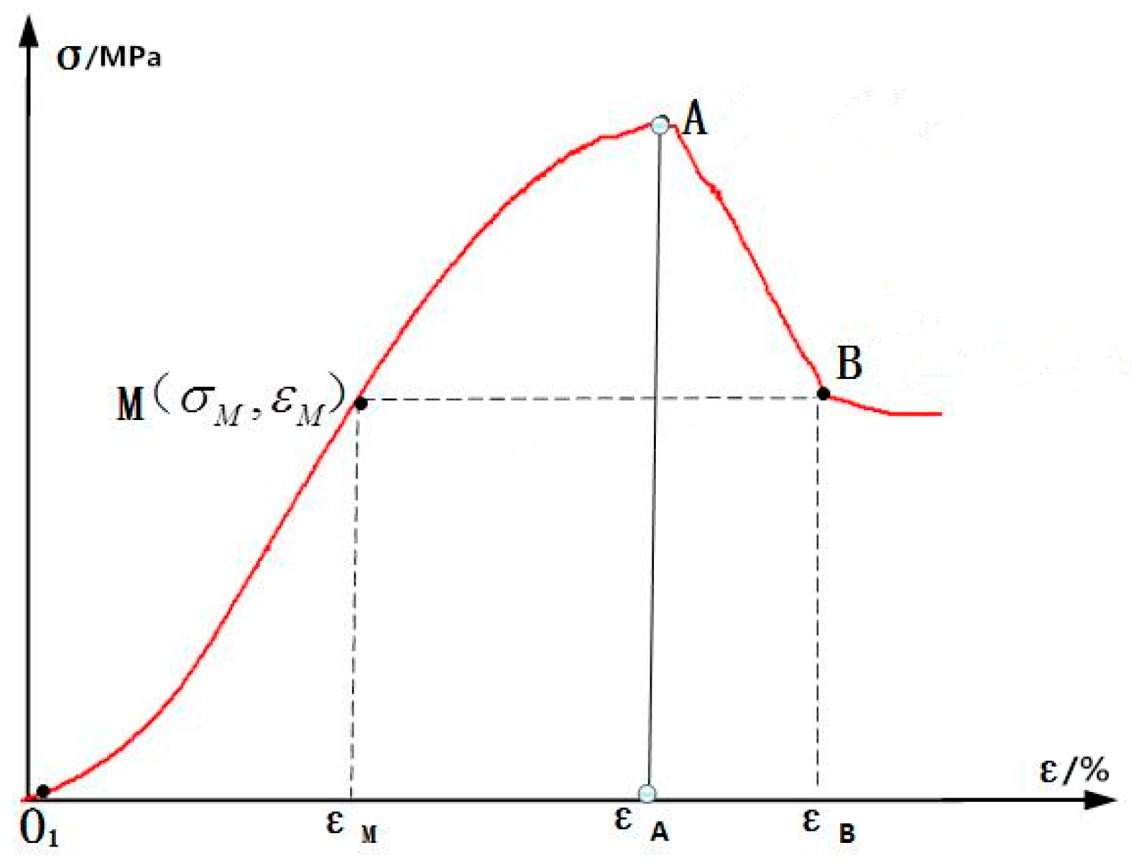
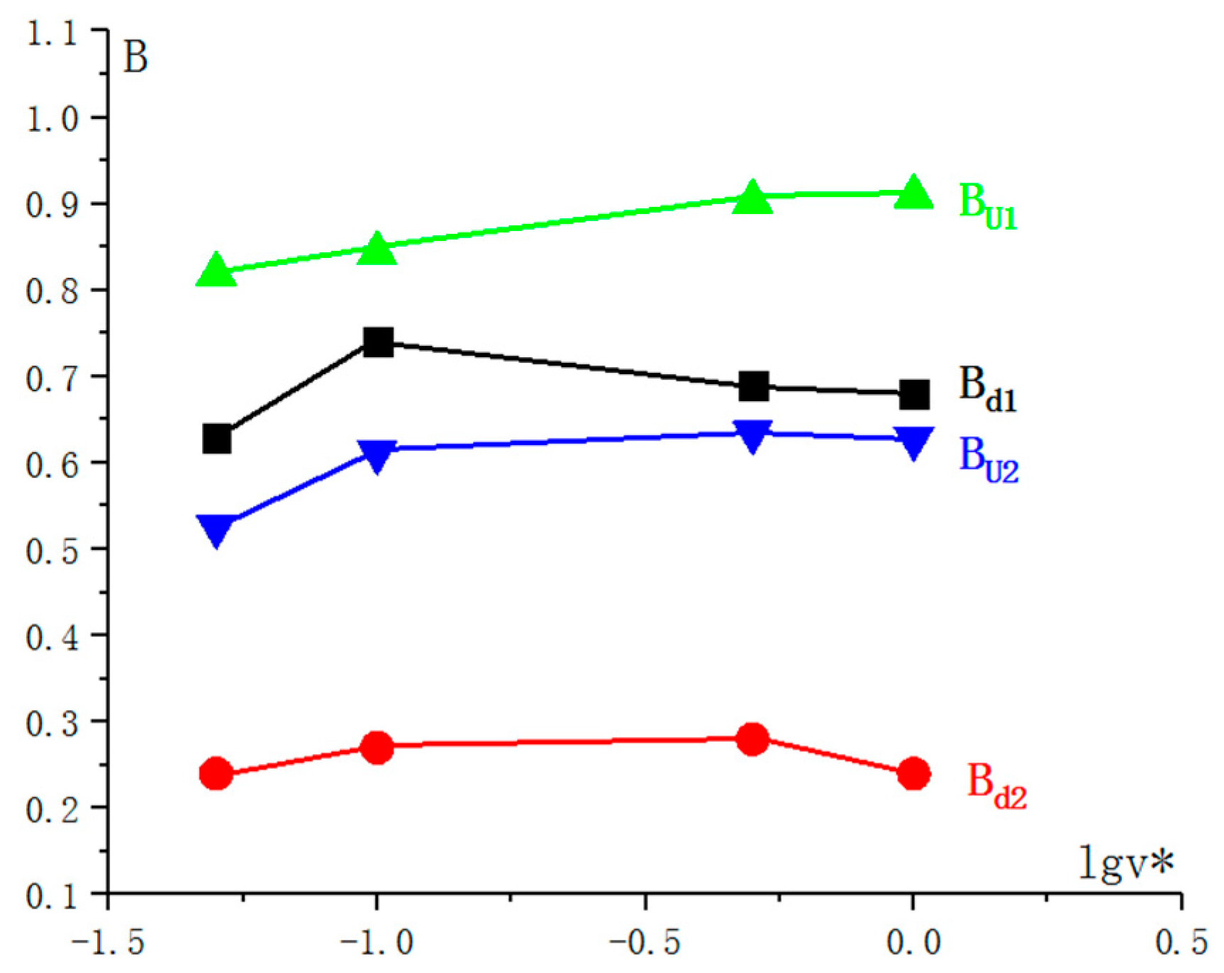
4.2.2. Proposal of Brittleness Evaluation Method Considering Unloading Conditions

Aiming at the above problems, the author proposes a brittleness evaluation method based on the unloading stress–strain curve. This method can consider the influence of different unloading rates on shale brittleness characteristics under the same confining pressure condition, and can be related to reservoir geology to analyze the brittleness of the reservoir further, providing a basis for the mining of preferred high brittle blocks and hydraulic fracturing.

After the unloading point in Figure 16, the magnitude of the deviatoric stress changes significantly at different unloading rates. Therefore, let the unloading point be U, them the unloading deformation modulus $E_U$ is proposed, which is taken from the amount of change between the deviatoric stress and the axial strain, between the peak point A and the unloading point U, that is, the discontinuous line at the unloading point in Figure 17 to the discontinuous line at the peak of the respective rate, which is:

$$E_U=({\sigma }_A-{\sigma }_U)/({\epsilon }_A-{\epsilon }_U)$$

(18)

where ${\sigma }_A$, ${\sigma }_U$ represents the intensity of the unloading point A and the peak point U, respectively, and ${\epsilon }_A$, ${\epsilon }_U$ represents the axial deformation of the point A and the point U, respectively. By calculation, the following table can be obtained (the sample number in the table omits the previous RF).

As the unloading rate increases in

Table 5. Unloading elastic modulus parameter table.

No.	1-15	4-11	2-7	3-3	4-2	2-5	3-4	3-5	2-2	2-9	4-5
$E_U$/GPa	15.74	38.73	22.59	26.50	41.25	44.90	58.40	50.50	42.68	65.38	52.60

, there is a significant increase from the lowest of 15.74 to 65.38 GPa in $E_U$. Therefore, the total elastic modulus based on both loading and unloading is proposed:

$$E_T=\varphi E+\gamma E_U$$

(19)

where $E_T$ is the total elastic modulus that considered both the loading and unloading, $E$ is the elastic modulus of the elastic section before the unloading point, $E_U$ is the unloading elastic modulus, $\varphi$ and $\gamma$ are the composite coefficient, and $\varphi +\gamma =1$. Then the Equation (18) is substituted into (19), and Equation (20) can be got.

$$E_T=\varphi E+\gamma ({\sigma }_A-{\sigma }_M)/({\epsilon }_A-{\epsilon }_M)$$

(20)

Because $M$ and $E$ are covered by $B_3$ in the literature [28] and $E$ is also covered in $B_1$, $B_1$, $B_2$ and $B_3$ are not independent. So they cannot be fitted to $B_{d1}$ and $B_{d2}$, then $B_3$ is deleted and $E_T$ is imported, and the brittleness evaluation index $B_{U1}$ and $B_{U2}$, which consider the loading and unloading part, can be established.

$$B_{U1}=\alpha \cdot exp\left\{\frac{\left[\varphi E+\gamma ({\sigma }_A-{\sigma }_M)/({\epsilon }_A-{\epsilon }_M)\right]\times ({\epsilon }_B-{\epsilon }_A)}{{\sigma }_r+{\sigma }_3-2\mu {\sigma }_3-\left[\varphi E+\gamma ({\sigma }_A-{\sigma }_M)/({\epsilon }_A-{\epsilon }_M)\right]{\epsilon }_A}\right\}+\beta \cdot (1-\frac{{\sigma }_r}{{\sigma }_A})$$

(21)

$$B_{U2}=exp\left\{\frac{\left[\varphi E+\gamma ({\sigma }_A-{\sigma }_M)/({\epsilon }_A-{\epsilon }_M)\right]({\epsilon }_B-{\epsilon }_A)}{{\sigma }_r+{\sigma }_3-2\mu {\sigma }_3-\left[\varphi E+\gamma ({\sigma }_A-{\sigma }_M)/({\epsilon }_A-{\epsilon }_M)\right]{\epsilon }_A}\right\}\times (1-\frac{{\sigma }_r}{{\sigma }_A})$$

(22)

where $\varphi +\gamma =1$, $\alpha +\beta =1$, the value of $\varphi$ and $\gamma$ can fully consider the size of the unloading rate and the difference of the unloading point and the value of $\alpha$ and $\beta$ can measure the different effects of stress and strain on the brittleness. Under the same confining pressure condition, ${\sigma }_3$ is generally a fixed value, $E$ is the elastic modulus of the elastic section before the unloading point, $\mu$ is the Poisson’s ratio of the pattern, and the remaining parameters can be read in the stress–strain curve.

4.2.3. Verification of the Brittleness Method and Comparison with Others

In the unloading test of this paper, due to the discrete difference of some samples, it has a small range of fluctuations of $E$, but $E_U$ has a more significant influence on the peak strength and brittleness of the unloading, so $\varphi$ is taken as 0.4 and $\gamma$ is taken as 0.6, which are more suitable for the actual situation during unloading. Then $\alpha$ and $\beta$ are both taken as 0.5, and $E_T$ can be calculated, as shown in

Table 6. Table of total elastic modulus.

No.	1-15	4-11	2-7	3-3	4-2	2-5	3-4	3-5	2-2	2-9	4-5
$E_T$/GPa	16.57	30.33	20.93	23.21	31.43	34.35	42.06	37.53	32.55	46.49	38.37

.

Then $E_T$ can be substituted into Equations (21) and (22), and the brittleness index $B_{U1}$ and $B_{U2}$ can be got.

From the comparison of the new methods and Hou’s method in Figure 17 and

Table 7. Table of the brittleness indicator parameter.

No.	1-15	4-11	2-7	3-3	4-2	2-5	3-4	3-5	2-2	2-9	4-5
$B_{U1}$	0.688	0.950	0.893	0.789	0.846	0.836	0.993	0.880	0.842	0.947	0.937
$B_{U2}$	0.326	0.725	0.716	0.504	0.617	0.508	0.759	0.637	0.545	0.649	0.692

, we can easily obtain that there are fluctuations between $B_{U1}$ and $B_{U2}$, which means they cannot characterize the brightness of the shale during the unloading. The average value of $B_{U1}$ and $B_{U2}$ can be calculated and obtained at each unloading rate, the average values of $B_{U1}$ at 0.05, 0.1, 0.5, and 1.0 MPa/s are: 0.819, 0.843, 0.903, and 0.909, respectively. It has a good brittleness characterization with the unloading damage and parameter changes in Chapter 3, and the feasibility of the brittleness evaluation method is verified. The average values of $B_{U2}$ at 0.05, 0.1, 0.5, and 1.0 MPa/s are 0.526, 0.612, 0.635, and 0.628. As the unloading rate increases, the overall trend of $B_{U2}$ shows an upward trend and there is a small fluctuation at the unloading rate of 1.0 MPa/s. $B_{U2}$ can also characterize the rock sample at different unloading rates, but it is weaker than the characterization of $B_{U1}$.

5. Conclusions

In this paper, the axial compression loading and confining pressure unloading test is carried out under the confining pressure of 60 MPa. The relationship between the unloading rate and the mechanical characteristics of the shale is discussed, also the brittleness of shale under the unloading path are analyzed. The following conclusions are obtained:

(1)

With the increase of unloading rate $v^{*}$, the axial strain and radial strain increases, the radial strain is more significant, and the volumetric strain is reduced gradually, which shows that the dilatancy is weaker. The unloading rate has a strengthening effect on the peak deviatoric stress and has a weakening effect on the residual deviatoric stress and the confining pressure, and there is a typical linear relationship between them. The modulus of elasticity decreases and the logarithm of the peak intensity has a significant linear relationship with the logarithm of the strain rate.

(2)

When $v^{*}$ is 0.05 MPa/s, the shale failure mode is mild, which is a typical single slope shear failure. When $v^{*}$ is 1.0 MPa/s, the shale fracture morphology is more complicated, the shear fracture surface is increased, and some bedding surface cracks. There are fine vertical distribution cracks between the fracture surfaces, and the shale fracture is sufficient, which shows the simultaneous development of multiple shear zones and synchronous cracking inside the layers, resulting in the overall instability of the shale.

(3)

The brittleness evaluation methods are summarized as a total of 33 kinds, and the brittleness of shale samples is well characterized by the brittleness index $B_{d1}$ and $B_{d2}$ during the loading process, they decrease continuously with the increase of confining pressure, which plays a good role in the characterization of the uniaxial failure and the triaxial failure. What is more, compared with $B_{d1}$, the numerical range of $B_{d2}$ is larger, and the high brittleness characteristics of shale samples under uniaxial compression can be highlighted, which proves the effective application of the method in triaxial loading test.

(4)

Aiming at the shortage of $B_{d1}$ and $B_{d2}$ during the unloading process, this paper proposes a brittleness evaluation method based on the unloading stress–strain curve, which can consider the influence of different unloading rates, and there is a good brittleness characterization between the unloading damage and parameter changes of $B_{U1}$ and $B_{U2}$. This can be related to reservoir geology to analyze the brittleness of the reservoir further, providing a basis for the mining of preferred high brittle blocks and hydraulic fracturing.

The following research will continue to focus on the unloading rate, explore the shale unloading test at different bedding angles under different confining pressure conditions, and deeply explore the shale unloading mechanism.

References

1. Guo, X.S. Rules of two-factor enrichment for marine shale gas in Southern China—Understanding from the Longmaxi formation shale gas in Sichuan basin and its surrounding area. Acta Geol. Sin. 2014, 88, 1209–1218. (In Chinese) [Google Scholar] [CrossRef]
2. Lyu, Q.; Ranjith, P.G.; Long, X.P.; Ji, B. Experimental investigation of mechanical properties of black shales after CO2-water-rock interaction. Materials 2016, 9, 663. [Google Scholar] [CrossRef] [PubMed]
3. Kim, K.; Choe, J. Hydraulic Fracture Design with a Proxy Model for Unconventional Shale Gas Reservoir with Considering Feasibility Study. Energies 2019, 12, 220. [Google Scholar] [CrossRef]
4. Energy Information Administration. Shale Gas Production Drives World Natural Gas Production Growth. 2016. Available online: https://www.eia.gov/todayinenergy/detail.php?id=27512 (accessed on 15 August 2016).
5. Huo, L.; Yang, C.H.; Liu, J.X.; Mao, H.J.; Huang, W.G. Experimental research on the failure of mudstone cap rock of Western Hubei-Eastern Chongqing suffered uplift and erosion. Chin. J. Undergr. Space Eng. 2018, 14, 33–42. (In Chinese) [Google Scholar]
6. Huo, L.; Yang, C.H.; Mao, H.J.; Liu, J.X.; Yuan, X.S. Experimental research on mechanical properties of western Hubei-Eastern Chongqing carbonaceous shale cap rock under unloading stress path. Chin. J. Rock Mech. Eng. 2016, a0135, 2898–2906. (In Chinese) [Google Scholar] [CrossRef]
7. Cao, C.R.; Han, C.H.; Zheng, D.R. Impact of structural changes on reservoir preservation. Mar. Geol. Quat. Geol. 2003, 23, 95–98. (In Chinese) [Google Scholar] [CrossRef]
8. Li, J.Q.; Gao, Y.Q.; Hua, C.X.; Xia, Z.L. Enlightenment from the experience of shale gas exploration in North America to the establishment of an evaluation system for marine shale gasification area in South China. Pet. Geol. Recovery Effic. 2014, 21, 23–27. (In Chinese) [Google Scholar] [CrossRef]
9. Dewhurst, D.N.; Hennig, A.L. Geomechanical properties related to top seal leakage in the Carnarvon Basin, Northwest Shelf, Australia. Pet. Geosci. 2003, 9, 255–263. [Google Scholar] [CrossRef]
10. Lewis, H.; Olden, P.; Couples, G.D. Geomechanical simulations of top seal integrity. Nor. Pet. Soc. Spec. Publ. 2002, 11, 75–87. [Google Scholar] [CrossRef]
11. Hermanrud, C.; Bols, H.M.; Teige, G.M. Seal failure related to basin-scale processes. AAPG Hedberg Series 2005, 1975, 13–22. [Google Scholar] [CrossRef]
12. Teige, G.M.; Hermanrud, C.; Kløvjan, O.S.; Eliassen, P.E.; Løseth, H.; Gading, M. Evaluation of caprock integrity in the western (high-pressured) haltenbanken area—A case history based on analyses of seismic signatures in overburden rocks. Nor. Pet. Soc. Spec. Publ. 2002, 11, 233–242. [Google Scholar] [CrossRef]
13. Ogata, K.; Senger, K.; Braathen, A.; Tveranger, J. Fracture corridors as seal-bypass systems in siliciclastic reservoir-cap rock successions: Field-based insights from the Jurassic Entrada Formation (SE Utah, USA). J. Struct. Geol. 2014, 66, 162–187. [Google Scholar] [CrossRef]
14. Shukla, R.; Ranjith, P.G.; Choi, S.K.; Haque, A.; Yellishetty, M.; Hong, L. Mechanical behaviour of reservoir rock under brine saturation. Rock Mech. Rock Eng. 2013, 46, 83–93. [Google Scholar] [CrossRef]
15. Ingram, G.M.; Urai, J.L. Top-seal leakage through faults and fractures: The role of mudrock properties. Geol. Soc. Lond. Spec. Publ. 1999, 158, 125–135. [Google Scholar] [CrossRef]
16. Swansson, S.R.; Brown, W.S. An observation of loading path independence of fracture in rock. Int. J. Rock Mech. Min. Sci. Geomech. Abstr. 1971, 8, 277–281. [Google Scholar] [CrossRef]
17. Shimamoto, T. Confining pressure reduction experiments: A new method for measuring frictional strength over a wide range of normal stress. Int. J. Rock Mech. Min. Sci. Geomech. Abstr. 1985, 22, 227–236. [Google Scholar] [CrossRef]
18. Viktorov, S.D.; Kochanov, A.N. Investigation into the processes of rock sample unloading after blast loading. J. Min. Sci. 2004, 40, 160–164. [Google Scholar] [CrossRef]
19. Lau, J.S.O.; Chandler, N.A. Innovative laboratory testing. Int. J. Rock Mech. Min. Sci. 2004, 41, 1427–1445. [Google Scholar] [CrossRef]
20. Huang, R.Q.; Huang, D. Experimental research on affection laws of unloading rates on mechanical properties of Jinping marble under high geostress. Chin. J. Rock Mech. Eng. 2010, 29, 21–33. (In Chinese) [Google Scholar]
21. Huang, X.; Liu, Q.S.; Liu, B.; Liu, X.W.; Pan, Y.C.; Liu, J.P. Experimental study on the dilatancy and fracturing behavior of soft rock under unloading conditions. Int. J. Civ. Struct. Eng. 2017, 15, 1–28. [Google Scholar] [CrossRef]
22. Zhang, L.M.; Wang, Z.Q.; Shi, L. Experimental study of hard rock failure characteristic under unloading condition. Chin. J. Rock Mech. Eng. 2011, 30, 1230–1236. (In Chinese) [Google Scholar] [CrossRef]
23. Lv, Y.H.; Liu, Q.S.; Jiang, H. Study of mechanical deformation characteristics of granite in unloading experiments of high stress. Rock Soil Mech. 2010, 31, 337–344. (In Chinese) [Google Scholar] [CrossRef]
24. Wu, F.Q.; Liu, J.Y.; Liu, T.; Zhuang, H.Z.; Yan, C.G. A method for assessment of excavation damaged zone (EDZ) of a rock mass and its application to a dam foundation case. Eng. Geol. 2009, 104, 254–262. [Google Scholar] [CrossRef]
25. He, M.C.; Miao, J.L.; Feng, J.L. Rock burst process of limestone and its acoustic emission characteristics under true-triaxial unloading conditions. Int. J. Rock Mech. Min. Sci. 2010, 47, 286–298. [Google Scholar] [CrossRef]
26. Hatheway, A.W. The complete ISRM suggested methods for rock characterization, testing, and monitoring: 1974–2006. Environ. Eng. Geol. 2009, 15, 47–48. [Google Scholar] [CrossRef]
27. Hou, Z.K.; Yang, C.H.; Wei, X.; Wang, L.; Wei, Y.L.; Xu, F.; Wang, H. Experimental study on the brittle characteristics of Longmaxi formation shale. J. China Coal Soc. 2016, 41, 1188–1196. (In Chinese) [Google Scholar] [CrossRef]
28. Hou, Z.K.; Yang, C.H.; Wang, L.; Xu, F. Evaluation Method of Shale Brittleness Based on Indoor Experiments. J. Northeast. Univ. Nat. Sci. 2016, 37, 1496–1501. (In Chinese) [Google Scholar] [CrossRef]
29. Altindag, R. The evaluation of rock brittleness concept on rotary blast hold drills. J. S. Afr. Inst. Min. Metall. 2002, 102, 61–66. [Google Scholar]
30. Hucka, V.; Das, B. Brittleness determination of rocks by different methods. Int. J. Rock Mech. Min. Sci. Geomech. Abstr. 1974, 11, 389–392. [Google Scholar] [CrossRef]
31. Honda, H.; Sanada, Y. Hardness of coal. Fuel 1956, 35, 451–461. [Google Scholar]
32. Quinn, J.B.; Quinn, D.G. Indentation brittleness of ceramics: A fresh approach. J. Mater. Sci. 1997, 32, 4331–4346. [Google Scholar] [CrossRef]
33. Lawn, B.; Marshall, D. Hardness, toughness, and brittleness: An indentation analysis. J. Am. Ceram. Soc. 1979, 62, 347–350. [Google Scholar] [CrossRef]
34. Azant, Z.P.; Kazemi, M.T. Determination of fracture energy, process zone length and brittleness number from size effect, with application to rock and concrete. Int. J. Fract. 1990, 44, 111–131. [Google Scholar] [CrossRef]
35. Hajiabdolmajid, V.; Kaiser, P. Brittleness of rock and stability assessment in hard rock tunneling. Tunn. Undergr. Space Eng. 2003, 18, 35–48. [Google Scholar] [CrossRef]
36. Copur, H. Theoretical and Experimental Studies of Rock Cutting with Drag Bits Toward the Development of a Performance Prediction Model for Roadheaders. Ph.D Thesis, Colorado School of Mines, Golden, CO, USA, 1999. [Google Scholar]
37. Yagiz, S. An investigation on the relationship between rock strength and brittleness. In Proceedings of the 59th Geological Congress of Turkey, Ankara, Turkey, 20–24 March 2006; MTA General Directory Press: Ankara, Turkey, 2006. [Google Scholar]
38. Blindheim, O.T.; Bruland, A. Boreability testing. Nor. TBM Tunn. 1998, 30, 29–34. [Google Scholar]
39. Protodyakonov, M.M. Mechanical properties and drillability of rocks. In Proceedings of the 5th Symposium Rock Mechanics, University of Minnesota, Minneapolis, MN, USA, May 1962. [Google Scholar]
40. Rickman, R.; Mullen, M.J.; Petre, J.E.; Grieser, W.V.; Kundert, D. A practical use of shale petrophysics for stimulation design optimization: All shale plays are not clones of the Barnett Shale. In Proceedings of the SPE Annual Technical Conference and Exhibition, Denver, CO, USA, 21–24 September 2008; Society of Petroleum Engineers: Denver, CO, USA, 2008. [Google Scholar]
41. Jarvie, D.M.; Hill, R.J.; Ruble, T.E.; Pollastro, R.M. Unconventional shale-gas systems: The Mississippian Barnett Shale of north-central Texas as one model for thermogenic shale-gas assessment. AAPG Bull. 2007, 91, 475–499. [Google Scholar] [CrossRef]
42. Heng, S.; Yang, C.H.; Li, Z.; Wang, L.; Hou, Z.K. Shale brittleness estimation based on energy dissipation. J. Cent. South Univ. Nat. Sci. 2016, 47, 577–585. (In Chinese) [Google Scholar] [CrossRef]
43. Li, Q.H.; Chen, M.; Jin, Y.; Wang, F.P.; Hou, B.; Zhang, B.W. Indoor evaluation method for shale brittleness and improvement. Chin. J. Rock Mech. Eng. 2012, 31, 1680–1685. (In Chinese) [Google Scholar]
44. Aubertin, M.; Gill, D.E.; Simon, R. On the use of the brittleness index modified (BIM) to estimate the post-peak behavior of rocks. In Proceedings of the 1st North American Rock Mechanics Symposium, Austin, TX, USA, 1–3 June 1994; American Rock Mechanics Association: Austin, TX, USA, 1994. [Google Scholar]
45. Feng, T.; Xie, X.B.; Wang, W.X.; Pan, C.L. Brittleness of rock and brittleness coefficient describing rockburst tendency. Min. Metall. Eng. 2000, 20, 18–19. (In Chinese) [Google Scholar]
46. George, E.A. Brittle failure of rock material-test results and constitutive models. AA Balkema/Rotterdam/Brolkfield 1995, 2, 123–128. [Google Scholar] [CrossRef]
47. Bishop, A.W. Progressive failure with special reference to the mechanism causing it. Proc. Geotech. Conf. Oslo 1967, 2, 142–150. [Google Scholar]
48. Stavrogin, A.N.; Tarasov, B.G. Experimental Physics and Rock Mechanics; CRC Press: Boca Raton, FL, USA, 2001. [Google Scholar]
49. Zhou, H.; Meng, F.Z.; Zhang, C.Q.; Xu, R.C.; Lu, J.J. Quantitative evaluation of rock brittleness based on stress–strain curve. Chin. J. Rock Mech. Eng. 2014, 33, 1114–1122. (In Chinese) [Google Scholar] [CrossRef]
Figure 1. Part of the samples.
Energies 12 01779 g001
Figure 2. XRD mineral diffraction pattern of the shale sample.
Energies 12 01779 g002
Figure 3. Scanning of microscopic electron microscopy at 10 and 2 μm.
Energies 12 01779 g003
Figure 4. Schematic diagram of the MTS test machine structure.
Energies 12 01779 g004
Figure 5. Triaxial stress–strain curve of the samples.
Energies 12 01779 g005
Figure 6. Fitting curve of σ 1 σ 3 .
Energies 12 01779 g006
Figure 7. Triaxial unloading curve.
Energies 12 01779 g007
Figure 8. Deviatoric stress–strain curve and partial amplification curve.
Energies 12 01779 g008
Figure 9. Comparison of triaxial loading and unloading stress–strain curves and partial amplification curve.
Energies 12 01779 g009
Figure 10. A logarithmic fitting curve of deviatoric stress and unloading rate.
Energies 12 01779 g010
Figure 11. A logarithmic fitting curve of confining pressure and unloading rate.
Energies 12 01779 g011
Figure 12. A logarithmic fit curve of residual strength and unloading rate.
Energies 12 01779 g012
Figure 13. Damage morphologies of shale specimens under different unloading rates.
Energies 12 01779 g013aEnergies 12 01779 g013b
Figure 14. Stress–strain curve of brittle rock [27].
Energies 12 01779 g014
Figure 15. Brittleness stress–strain curve of shale samples under different unloading rates.
Energies 12 01779 g015
Figure 16. Magnification of typical stress–strain curves for four unloading rates.
Energies 12 01779 g016
Figure 17. Comparison of the methods.
Energies 12 01779 g017