Optimal Operational Scheduling of Reconfigurable Multi-Microgrids Considering Energy Storage Systems


Abstract
:1. Introduction
- A one-leader multi-follower-type bi-level model considering ESSs in an uncertain environment is proposed,
- An optimal day-ahead scheduling of multi-MG distribution systems is proposed considering DR and hourly reconfiguration actions,
- Modelling the DSO’s decision-making problem which is affected not only by the exchanged power between DSO and each MG as a mutual decision variable but also by the reactions of interconnected MGs in an hourly reconfigurable environment.
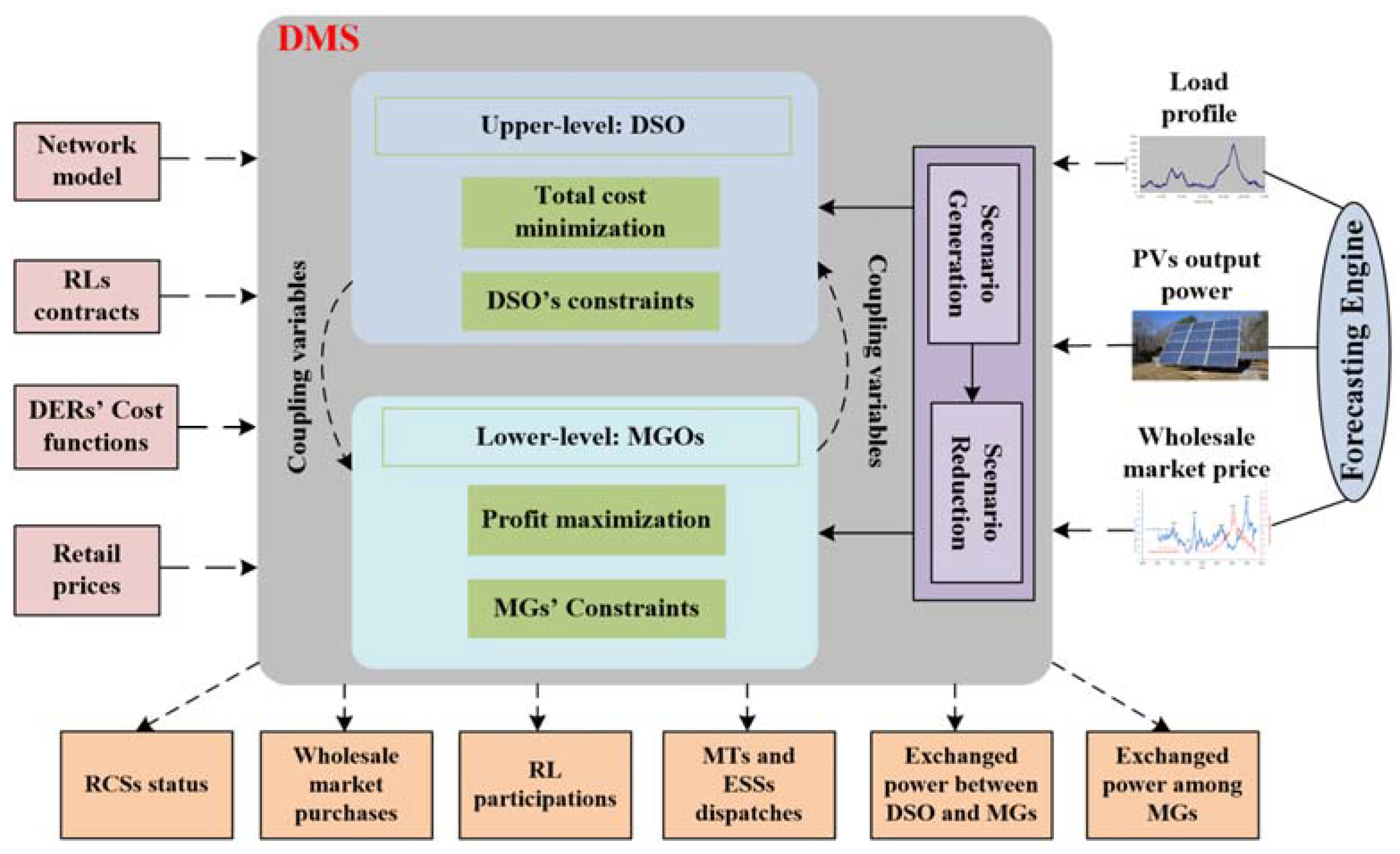
2. Conceptual Framework of the Proposed DMS
Uncertainty Modelling
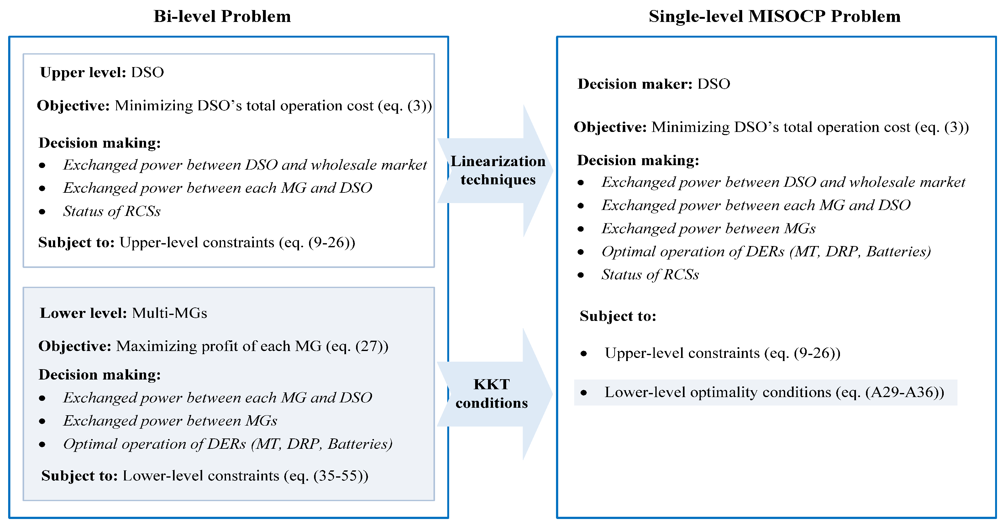
3. Bi-Level Formulation of the Optimization Problem
3.1. Upper-Level: DSO
- Distribution power flow equations:
- Voltage limits constraints:
- Exchanged power limit with the wholesale market:
- Line current limits:
- Network radiality:
- Number of switching actions:
- Exchanged power limit between MGs and DSO:
3.2. Lower-Level: Multi-MGs
- Operation limit of MT:
- Exchanged power limit with DSO:
- Exchanged power limit between MGs:
- Limits on operation of ESSs:
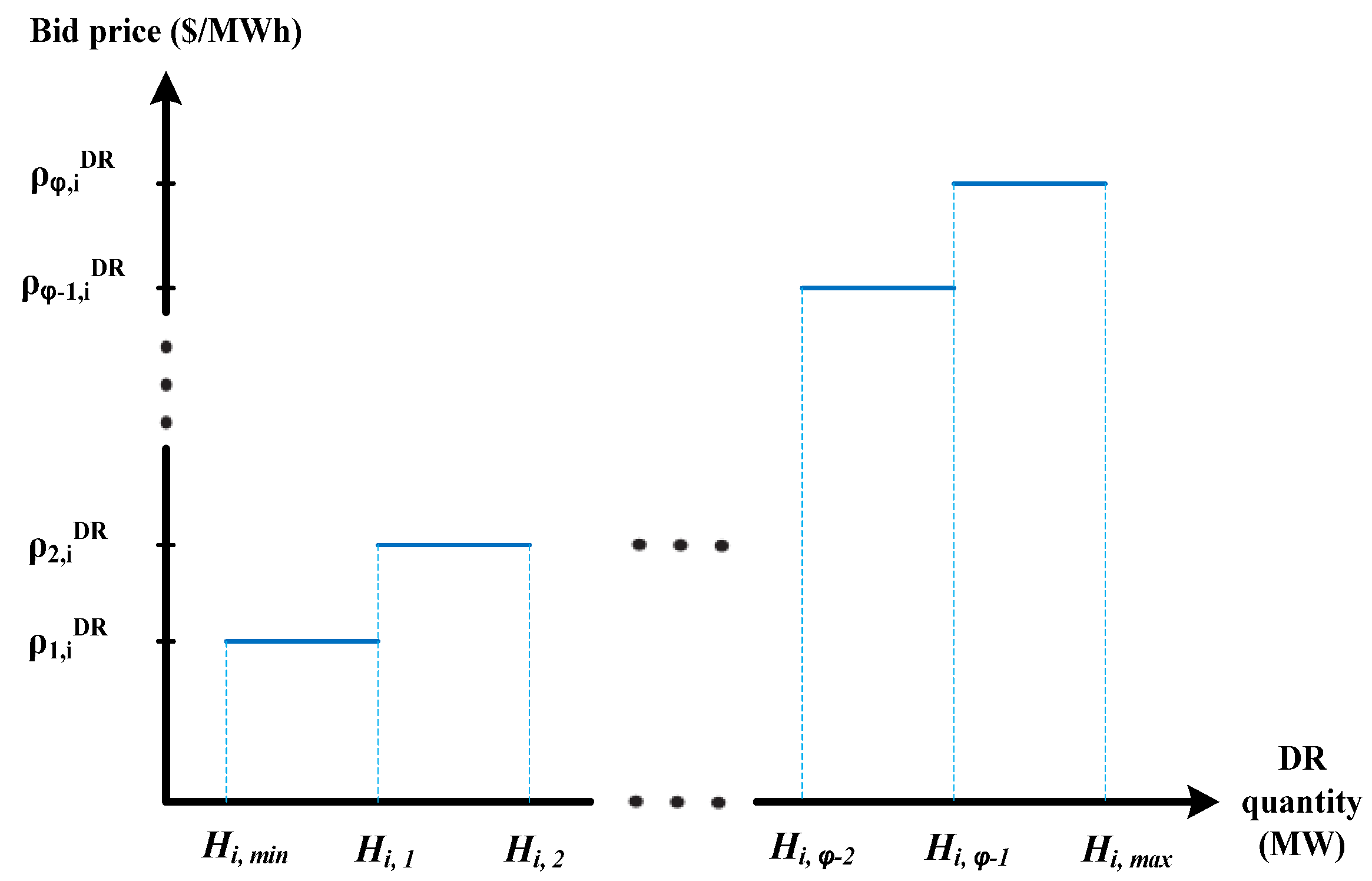
- DR program limits:
- Power balance for pth MG:
3.3. Solution Methodology
3.4. Verification of Nash Equilibrium
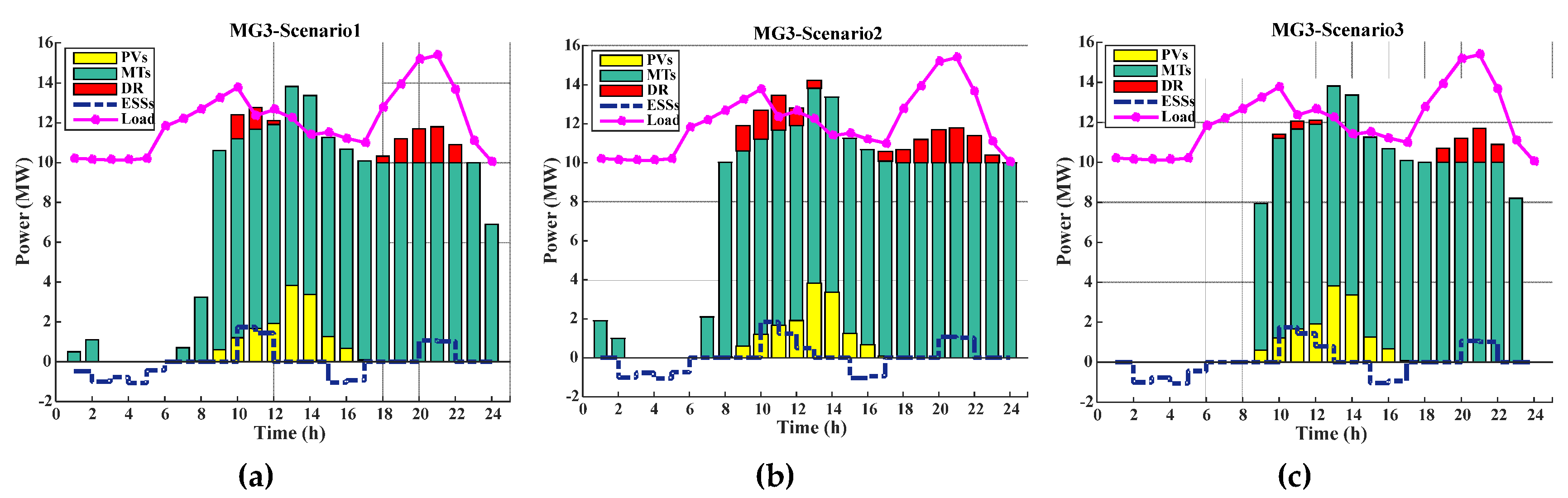
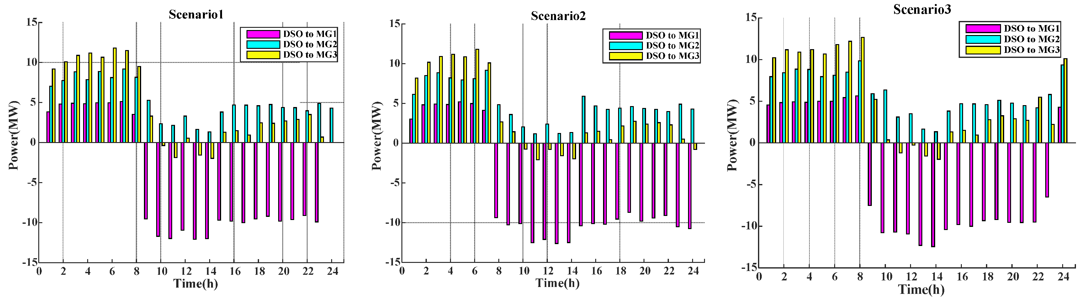
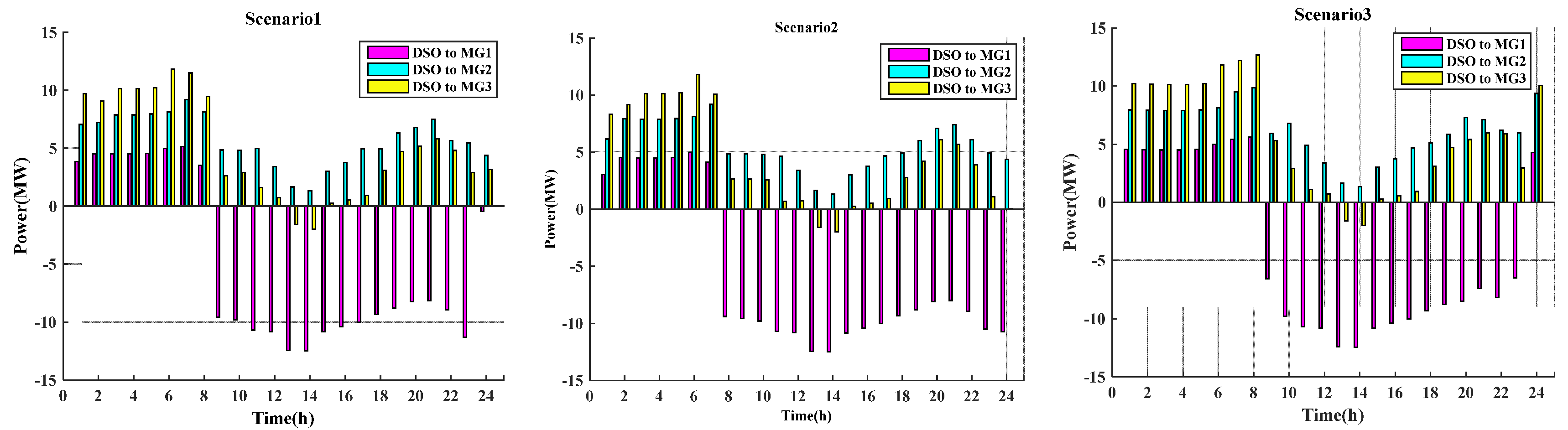
4. Test and Results
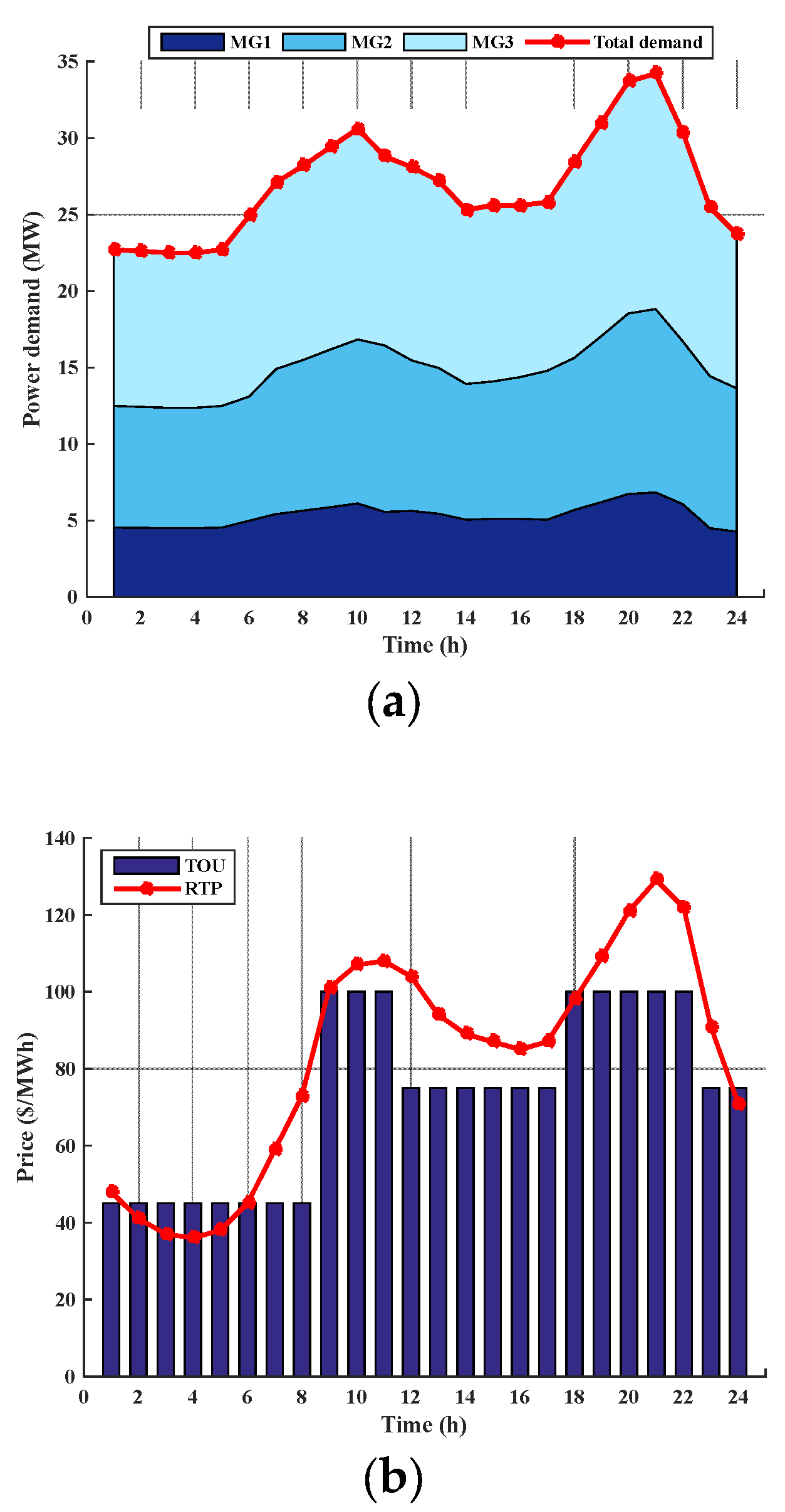
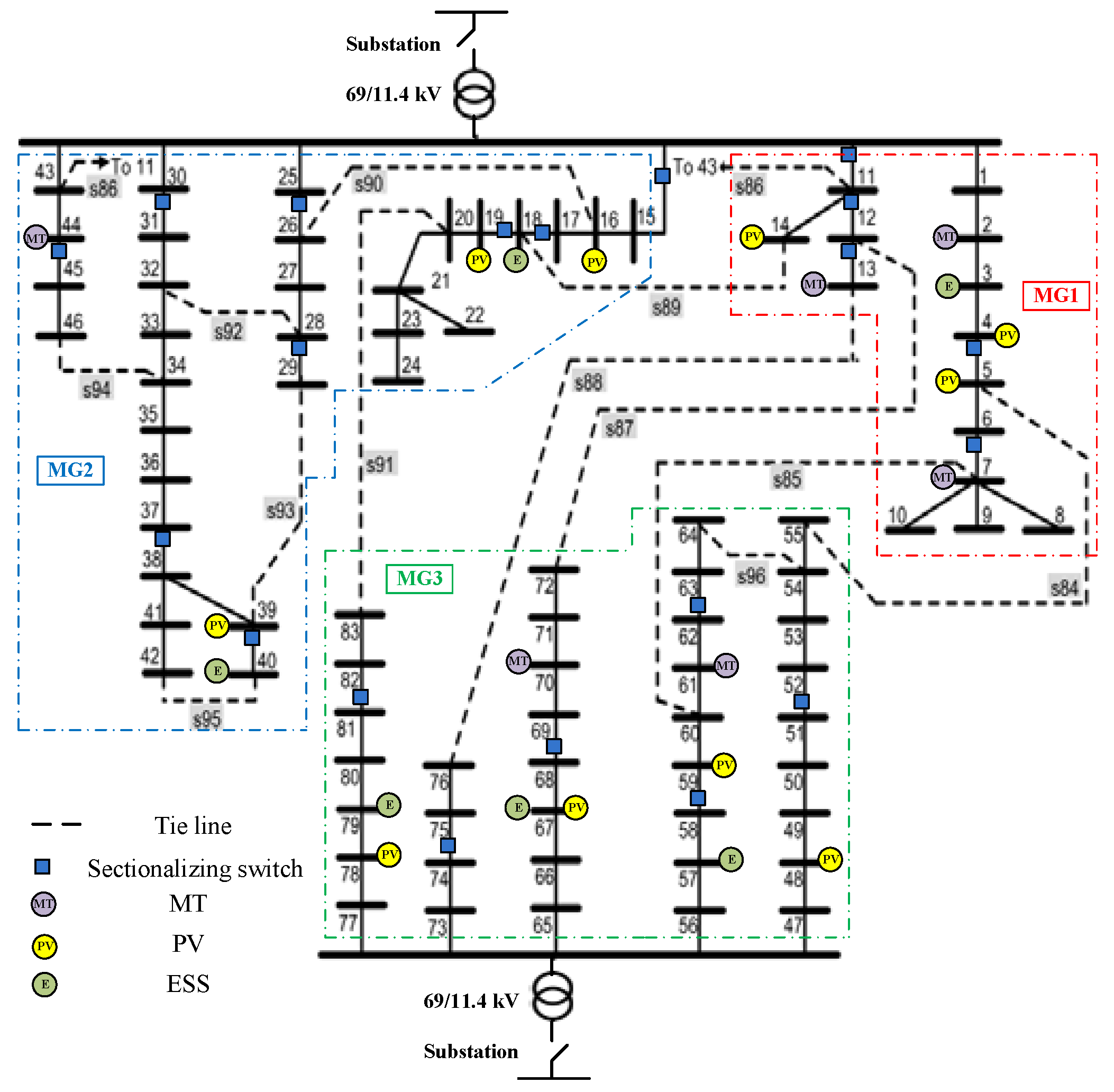
4.1. Case study
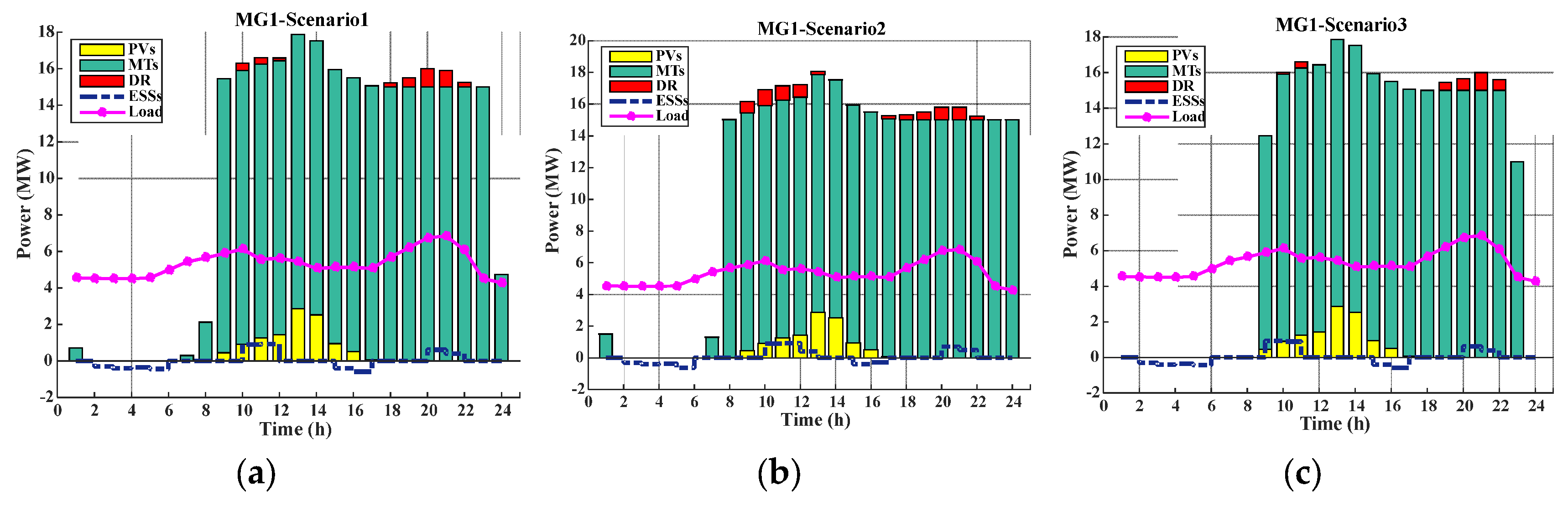
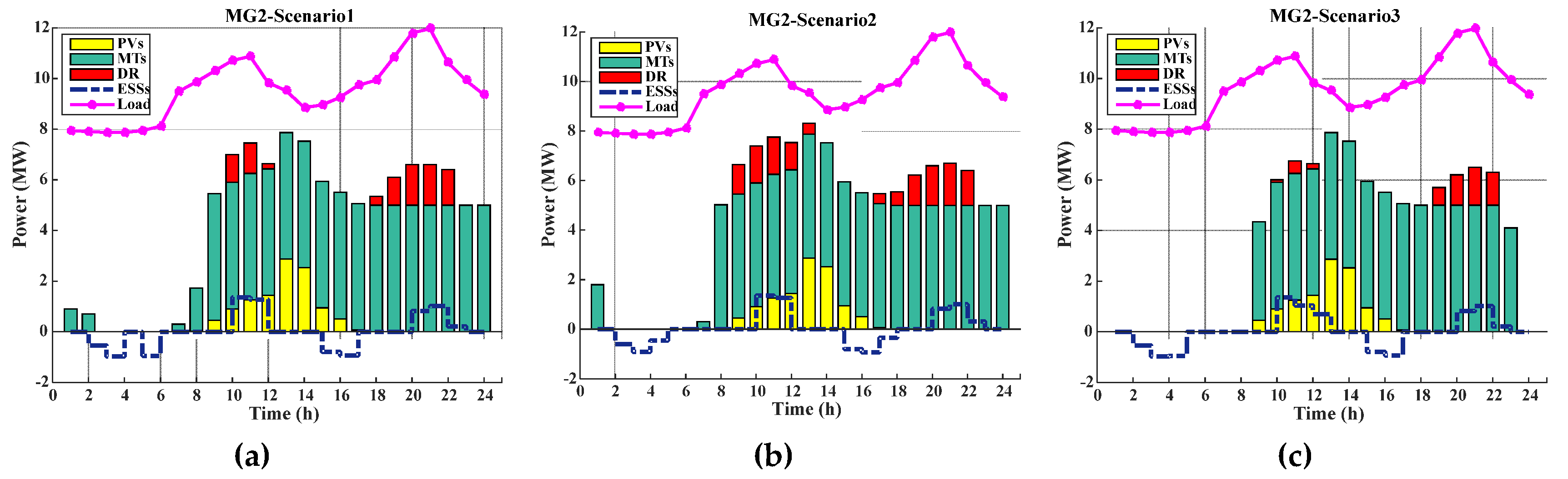
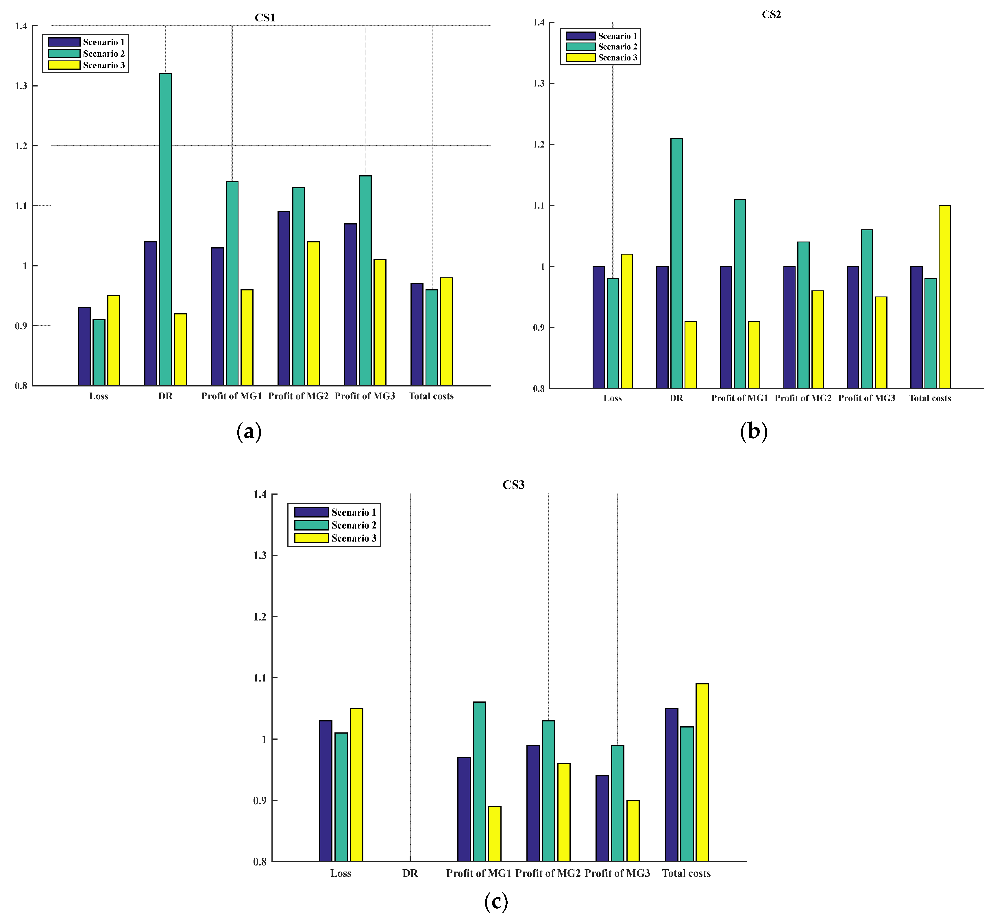
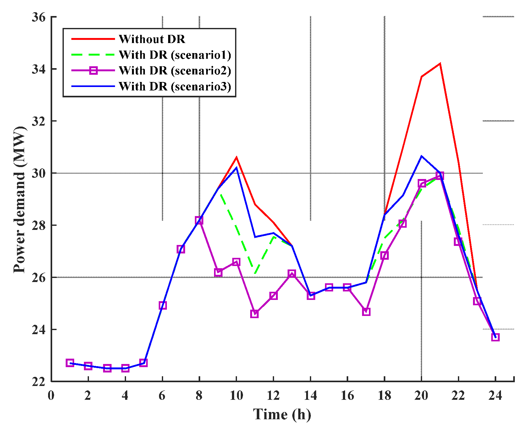
4.2. Simulation results
5. Conclusions
Author Contributions
Funding
Conflicts of Interest
Appendix A
Nomenclature
| Parameters | |
| Admittance between bus i and ground. | |
| Charging/Discharging efficiency of ESS i. | |
| Conductance/ susceptance of bus i. | |
| Day-ahead wholesale market electricity price at time t ($/MWh). | |
| Impedance of branch ij. | |
| Initial energy storage of ESS i (MWh). | |
| Local market price ($/MWh). | |
| Minimum down/up time for MT i. | |
| Number of generated scenarios for wholesale market price/ PV output power/ demanded load. | |
| Offered price of DR program for load curtailment in step ξ at time t ($/MWh). | |
| Operation & maintenance cost coefficient of Energy Storage System (ESS) i ($/MWh). | |
| Operation & maintenance cost coefficient of MT i ($/MWh). | |
| Operation & maintenance cost coefficient of PV i ($/MWh). | |
| Price for power losses ($/MWh). | |
| Price of each switching operation ($). | |
| Probability of scenarios for wholesale market price/ PV output power/ demanded load. | |
| Ramp-up/ramp-down rate of MT i. | |
| Resistance/reactance of branch ij. | |
| Variables | |
| Amount of accepted load curtailment for DR program in step ξ of bus i. | |
| Apparent power of branch ij at time t. | |
| Auxiliary variables for linear modelling of minimum down/up time limits. | |
| Auxiliary variable used for linearization of the complementary conditions. | |
| Binary variable for the charging /discharging status of ESS i at time t (0: when ESS i is not in the charging or discharging mode). | |
| STD | Standard deviation |
| TOU | Time-of-use |
| Indices and sets | |
| Index for On-time/OFF-time limits modelling. | |
| ). | |
| ). | |
| ). | |
| ). | |
| ). | |
| ). | |
| . | |
| Set of scenarios. | |
| Binary variable for the status of MT i at time t (0: when MT i is OFF). | |
| Binary variable for the status of RCS sw at time t (0: when the related switch is opened) | |
| Cost of exchanging power between DSO and MGs ($). | |
| Cost of exchanging power with wholesale market at time t ($). | |
| Cost of switching actions for RCSs at time t ($). | |
| Current of branch ij at time t (kA). | |
| Curtailed power of DR for bus i at time t (MW). | |
| Day-ahead power purchased/sold from/to wholesale market at time t by DSO (MW). | |
| Dual variable. | |
| Energy storage of ESS i at time t (MWh). | |
| ESS i charge/discharge power at time t (MW). | |
| Greater than or equal to zero constraints. | |
| Lagrangian function of pth lower-level problem related to MG p. | |
| Number of buses in the border of MG p at time t. | |
| Output active power of MT i at time t (MW). | |
| Output power of PV i at time t (MW). | |
| Output reactive power of MT i at time t (MVAR). | |
| includes loads, PVs, MTs, DR programs and exchanged power between MGs and DSO). | |
| Squared voltage/current magnitude of branch ij. | |
| The net injected active/reactive power at bus i. | |
| Total electrical load of bus i at time t (MW). | |
| Transmitted power from MG p to DSO/ from DSO to MG p (MW). | |
| Transmitted power from MG p to MG q at time t (MW). | |
| Voltage magnitude of bus i at time t. | |
References
- Kim, M.S.; Haider, R.; Cho, G.J.; Kim, C.H.; Won, C.Y.; Chai, J.S. Comprehensive Review of Islanding Detection Methods for Distributed Generation Systems. Energies 2019, 12, 837. [Google Scholar] [CrossRef]
- Holjevac, N.; Capuder, T.; Kuzle, I. Defining key parameters of economic and environmentally efficient residential microgrid operation. Energy Procedia 2017, 105, 999–1008. [Google Scholar] [CrossRef]
- Khodaei, A. Provisional microgrid planning. IEEE Trans. Smart Grid 2017, 8, 1096–1104. [Google Scholar] [CrossRef]
- Quashie, M.; Marnay, C.; Bouffard, F.; Joós, G. Optimal planning of microgrid power and operating reserve capacity. Appl. Energy 2018, 210, 1229–1236. [Google Scholar] [CrossRef]
- Esmaeili, S.; Jadid, S. Economic-Environmental Optimal Management of Smart Residential Micro-Grid Considering CCHP System. Electr. Power Syst. Res. 2019, 1–15. [Google Scholar] [CrossRef]
- Uski, S.; Rinne, E.; Sarsama, J. Microgrid as a Cost-Effective Alternative to Rural Network Underground Cabling for Adequate Reliability. Energies 2018, 11, 1978. [Google Scholar] [CrossRef]
- Meirinhos, J.L.; Rua, D.E.; Carvalho, L.M.; Madureira, A.G. Multi-temporal Optimal Power Flow for voltage control in MV networks using Distributed Energy Resources. Electr. Power Syst. Res. 2017, 146, 25–32. [Google Scholar] [CrossRef]
- Gutiérrez-Alcaraz, G.; Galván, E.; González-Cabrera, N.; Javadi, M.S. Renewable energy resources short-term scheduling and dynamic network reconfiguration for sustainable energy consumption. Renew. Sustain. Energy Rev. 2015, 52, 256–264. [Google Scholar] [CrossRef]
- Faria, P.; Spínola, J.; Vale, Z. Distributed Energy Resources Scheduling and Aggregation in the Context of Demand Response Programs. Energies 2018, 11, 1987. [Google Scholar] [CrossRef]
- Marvasti, A.K.; Fu, Y.; DorMohammadi, S.; Rais-Rohani, M. Optimal operation of active distribution grids: A system of systems framework. IEEE Trans. Smart Grid 2014, 5, 1228–1237. [Google Scholar] [CrossRef]
- Lv, T.; Ai, Q.; Zhao, Y. A bi-level multi-objective optimal operation of grid-connected microgrids. Electr. Power Syst. Res. 2016, 131, 60–70. [Google Scholar] [CrossRef]
- Feijoo, F.; Das, T.K. Emissions control via carbon policies and microgrid generation: A bilevel model and Pareto analysis. Energy 2015, 90, 1545–1555. [Google Scholar] [CrossRef]
- Aghajani, S.; Kalantar, M. Operational scheduling of electric vehicles parking lot integrated with renewable generation based on bilevel programming approach. Energy 2017, 139, 422–432. [Google Scholar] [CrossRef]
- Sandgani, M.R.; Sirouspour, S. Energy management in a network of grid-connected microgrids/nanogrids using compromise programming. IEEE Trans. Smart Grid 2018, 9, 2180–2191. [Google Scholar]
- Haddadian, H.; Noroozian, R. Multi-microgrids approach for design and operation of future distribution networks based on novel technical indices. Appl. Energy 2017, 185, 650–663. [Google Scholar] [CrossRef]
- Gazijahani, F.S.; Ravadanegh, S.N.; Salehi, J. Stochastic multi-objective model for optimal energy exchange optimization of networked microgrids with presence of renewable generation under risk-based strategies. ISA Trans. 2018, 73, 100–111. [Google Scholar] [CrossRef] [PubMed]
- Bahramara, S.; Moghaddam, M.P.; Haghifam, M.R. A bi-level optimization model for operation of distribution networks with micro-grids. Int. J. Electr. Power Energy Syst. 2016, 82, 169–178. [Google Scholar] [CrossRef]
- Bahramara, S.; Moghaddam, M.P.; Haghifam, M.R. Modelling hierarchical decision making framework for operation of active distribution grids. IET Gener. Transm. Distrib. 2015, 9, 2555–2564. [Google Scholar] [CrossRef]
- Jalali, M.; Zare, K.; Seyedi, H. Strategic decision-making of distribution network operator with multi-microgrids considering demand response program. Energy 2017, 141, 1059–1071. [Google Scholar] [CrossRef]
- Yu, M.; Hong, S.H. Supply–demand balancing for power management in smart grid: A Stackelberg game approach. Appl. Energy 2016, 164, 702–710. [Google Scholar] [CrossRef]
- Yu, M.; Hong, S.H. A Real-Time Demand-Response Algorithm for Smart Grids: A Stackelberg Game Approach. IEEE Trans. Smart Grid 2016, 7, 879–888. [Google Scholar] [CrossRef]
- Esmaeili, S.; Anvari-Moghaddam, A.; Jadid, S.; Guerrero, J.M. Optimal Operational Scheduling of Smart Microgrids Considering Hourly Reconfiguration. In Proceedings of the 2018 IEEE 4th Southern Power Electronics Conference (SPEC), Singapore, Singapore, 10–13 December 2018; pp. 1–6. [Google Scholar]
- Esmaeili, S.; Anvari-Moghaddam, A.; Jadid, S.; Guerrero, J.M. A Stochastic Model Predictive Control Approach for Joint Operational Scheduling and Hourly Reconfiguration of Distribution Systems. Energies 2018, 11, 1884. [Google Scholar] [CrossRef]
- Chen, S.; Hu, W.; Chen, Z. Comprehensive cost minimization in distribution networks using segmented-time feeder reconfiguration and reactive power control of distributed generators. IEEE Trans. Power Syst. 2016, 31, 983–993. [Google Scholar] [CrossRef]
- Anand, M.P.; Golshannavaz, S.; Ongsakul, W.; Rajapakse, A. Incorporating short-term topological variations in optimal energy management of MGs considering ancillary services by electric vehicles. Energy 2016, 112, 241–253. [Google Scholar] [CrossRef]
- Hemmati, M.; Mohammadi-Ivatloo, B.; Ghasemzadeh, S.; Reihani, E. Risk-based optimal scheduling of reconfigurable smart renewable energy based microgrids. Int. J. Electr. Power Energy Syst. 2018, 101, 415–428. [Google Scholar] [CrossRef]
- Gazijahani, F.S.; Salehi, J. Optimal bilevel model for stochastic risk-based planning of microgrids under uncertainty. IEEE Trans. Ind. Inform. 2018, 14, 3054–3064. [Google Scholar] [CrossRef]
- Shahmohammadi, A.; Sioshansi, R.; Conejo, A.J.; Afsharnia, S. Market equilibria and interactions between strategic generation, wind, and storage. Appl. Energy 2018, 220, 876–892. [Google Scholar] [CrossRef]
- Rostami, M.A.; Kavousi-Fard, A.; Niknam, T. Expected cost minimization of smart grids with plug-in hybrid electric vehicles using optimal distribution feeder reconfiguration. IEEE Trans. Ind. Inform. 2015, 11, 388–397. [Google Scholar] [CrossRef]
- Rabiee, A.; Sadeghi, M.; Aghaeic, J.; Heidari, A. Optimal operation of microgrids through simultaneous scheduling of electrical vehicles and responsive loads considering wind and PV units uncertainties. Renew. Sustain. Energy Rev. 2016, 57, 721–739. [Google Scholar] [CrossRef]
- Esmaeili, S.; Anvari-Moghaddam, A.; Jadid, S.; Guerrero, J.M. Optimal simultaneous day-ahead scheduling and hourly reconfiguration of distribution systems considering responsive loads. Int. J. Electr. Power Energy Syst. 2019, 104, 537–548. [Google Scholar] [CrossRef]
- CPLEX Optimization Subroutine Library Guide and Reference; ILOG Inc.: Incline Village, NV, USA, 2008.


| Parameter | Value | Parameter | Value |
|---|---|---|---|
| 250 | 71 | ||
| 36 | 11 | ||
| 20 | 8 | ||
| 15 | 0.95, 1.05 | ||
| 3.8 | 0, 5 | ||
| 1 | 8 |
| DR program | Buses |
|---|---|
| MG1 | 1, 4, 6, 7, 8, 12 |
| MG2 | 16, 17, 18, 22, 23, 28, 31, 32, 40, 45 |
| MG3 | 49, 50, 54, 59, 62, 63, 67, 68, 72, 80, 81, 82 |
| MG No. | DR Program [Quantity range* (MW)] & [Price** ($/MWh)] | |||
|---|---|---|---|---|
| MG1 | 0–0.2* | 0.2–0.5 | 0.5–0.7 | 0.7–1.1 |
| 94 ** | 97 | 102 | 112 | |
| MG2 | 0–0.2 | 0.2–0.8 | 0.8–1.4 | 1.4–1.7 |
| 91 | 97 | 104 | 116 | |
| MG3 | 0–0.2 | 0.2–0.7 | 0.7–1.3 | 1.3–1.8 |
| 92 | 96 | 102 | 114 | |
| Scenario 1 | Scenario 2 | Scenario 3 | |
|---|---|---|---|
| CS1 | Hourly reconfiguration, DR, ESSs, base prices | Hourly reconfiguration, DR, ESSs, 10% increment in prices | Hourly reconfiguration, DR, ESSs, 10% decrement in prices |
| CS2 | DR, ESSs, base prices | DR, ESSs, 10% increment in prices | DR, ESSs, 10% decrement in prices |
| CS3 | base prices | 10% increment in prices | 10% decrement in prices |
| Hour | Open RCSs | Hour | Open RCSs |
|---|---|---|---|
| 1 | 52-85-86-87-88-89-90-91-92-93-94-95-96 | 12–15 | 18-26-84-85-86-87-88-91-92-93-94-95-96 |
| 2–3 | 52-84-85-86-87-88-89-90-91-92-93-94-95 | 16–18 | 84-85-86-87-88-89-90-91-92-93-94-95-96 |
| 4–8 | 84-85-86-87-88-89-90-91-92-93-94-95-96 | 19–21 | 52-75-85-86-87-89-90-91-92-93-94-95-96 |
| 9–11 | 18-52-85-86-87-88-90-91-92-93-94-95-96 | 22–24 | 19-59-84-86-87-88-89-90-92-93-94-95-96 |
© 2019 by the authors. Licensee MDPI, Basel, Switzerland. This article is an open access article distributed under the terms and conditions of the Creative Commons Attribution (CC BY) license (http://creativecommons.org/licenses/by/4.0/).
Share and Cite
Esmaeili, S.; Anvari-Moghaddam, A.; Jadid, S. Optimal Operational Scheduling of Reconfigurable Multi-Microgrids Considering Energy Storage Systems. Energies 2019, 12, 1766. https://doi.org/10.3390/en12091766
Esmaeili S, Anvari-Moghaddam A, Jadid S. Optimal Operational Scheduling of Reconfigurable Multi-Microgrids Considering Energy Storage Systems. Energies. 2019; 12(9):1766. https://doi.org/10.3390/en12091766
Chicago/Turabian StyleEsmaeili, Saeid, Amjad Anvari-Moghaddam, and Shahram Jadid. 2019. "Optimal Operational Scheduling of Reconfigurable Multi-Microgrids Considering Energy Storage Systems" Energies 12, no. 9: 1766. https://doi.org/10.3390/en12091766
APA StyleEsmaeili, S., Anvari-Moghaddam, A., & Jadid, S. (2019). Optimal Operational Scheduling of Reconfigurable Multi-Microgrids Considering Energy Storage Systems. Energies, 12(9), 1766. https://doi.org/10.3390/en12091766