1. Introduction
In recent years, solar energy has become the second-largest energy source after wind energy among the renewable energy sources that are used for electricity production [
1]. The concentrating solar power (CSP), which uses either organic oil or molten salt as its heat transfer fluid (HTF) to absorb and transfer solar energy, is currently the most commercially attractive solar thermal-based power generation technology [
2].
To fill the generation gaps in intermittent solar energy, the CSP plant is generally integrated with thermal energy storage (TES), which enables the CSP plant to control its power output flexibly in the presence of solar uncertainty [
3]. Actually, the TES enables the CSP plant to be partly independent from constantly changing solar radiation [
4], reducing the short-term load variation and extending or shifting the power supply period [
5]. Therefore, the CSP plant is potentially capable of supplying the power on demand, participating in electricity markets by scheduling the power production throughout each day [
6], and providing ancillary services such as regulating the grid frequency [
7]. By participating in electricity markets, the revenue of the CSP plant can be significantly improved [
1]. For this reason, power scheduling is required to maximize the revenue, which is known as the decision-level power generation control [
8]. Additionally, when the CSP plant serves as the load-following power plant, it must be able to regulate the power output rapidly in response to the changing demand for power supply [
9].
The demand for the flexible operation of the CSP plant brings a high requirement to its execution-level dynamic control. The CSP plant must be able to rapidly adjust its power output in a wide operation range and simultaneously maintain the stability of the main steam pressure and temperature for safety and economic reasons. To achieve this goal, it is necessary to perform a thorough investigation of the system dynamic behavior, and on this basis find an appropriate execution-level control strategy for controlling power tracking.
Existing research works related to the execution-level control of CSP plants integrated with TES mainly focused on the control of the HTF temperature in collector field. Cirre et al. used a feedback linear control scheme to control the HTF temperature, which can reduce the influence of process nonlinearity [
10]. Gallego and Camacho proposed a state-space model predictive control to reject external disturbance on the HTF temperature [
11]. Alsharkawi and Rossiter developed an improved gain scheduling predictive control, incorporating a feed-forward strategy to improve the temperature control performance [
12]. Nevado Reviriego, Hernández-del-Olmo, and Álvarez-Barcia studied a nonlinear adaptive control scheme for the HTF temperature, which can cope with the time-varying nature of the process [
13].
However, few of these research works have focused on the execution-level power tracking control of CSP plants, which is even more challenging than the HTF temperature control. In fact, power tracking is not a stand-alone control problem. The control action that changes the power output can bring significant disturbances to the main steam (steam flowing into the turbine) pressure and temperature. Accelerating the power tracking rate can easily result in significant fluctuation in the main steam parameters, which imposes a negative effect on the safe and economic operation of the CSP plant. Furthermore, in CSP plants, the steam generator dynamics are much slower than the steam turbine dynamics, and it is challenging to coordinate the control of two systems with completely different response speeds.
Considering these issues, this paper proposes an execution-level power tracking control strategy for CSP plants that aims at achieving the dual tasks of fast power tracking and small fluctuation in the main steam parameters by coordinating the operation of the steam generator and the turbine. The heuristic PI control strategy with two operation modes, i.e., the fast power tracking mode (FT mode) and the smooth operation mode (SO mode), is first studied based on our knowledge about the process. However, each operation mode of heuristic PI can only satisfy one of the two control tasks. Therefore, the advanced model predictive control (MPC) strategy is further proposed to enhance the coordinating strategy and achieve both of the control tasks.
The remainder of this paper is organized as follows. The description and modeling of the CSP plant are presented in
Section 2.
Section 3 includes the transient analysis and process model identification. In
Section 4, the heuristic PI control strategy and the MPC strategy are formulated, and their control performance is evaluated.
Section 5 contains the conclusions.
2. Simulation Model of the CSP Plant
This section presents the simplified simulation model of a CSP plant with two-tank direct TES.
Figure 1 shows the simplified scheme of the plant considered in this study, and its working principle is described as follows. The HTF (orange line in
Figure 1) from the cold molten salt tank absorbs the solar radiation in the solar field, which comprises a set of single-axis tracking parabolic trough concentrators, and is then stored in the hot molten salt tank. In the meantime, the hot tank releases the stored HTF, which sequentially flows through the superheater, the boiler, and the economizer. In the economizer, the working fluid in the Rankine cycle is in liquid phase (blue line) and preheated close to its saturation temperature. In the boiler, the working fluid undergoes a phase change and evaporates from liquid to saturated steam. In the superheater, the saturated steam is further heated into superheated steam. Finally, the superheated steam (main steam) passes through the main steam valve and drives the steam turbine to produce electric power. To control the main steam temperature, an attemperator, which can spray feed water, is installed before the last-level superheater.
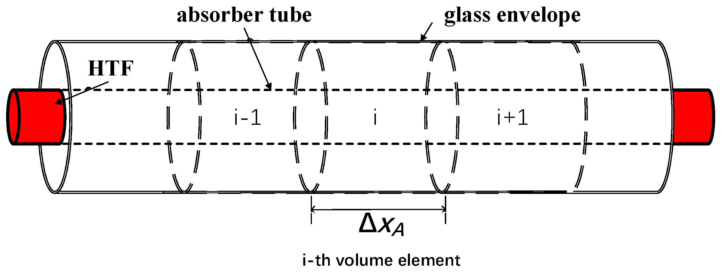
2.1. Solar Collector Model
The solar collector consists of a parabolic mirror, a glass envelope, and an absorber tube. The sunlight entering the mirror aperture is focused on the focal line, where the absorber tube is positioned. The absorber tube is enclosed by an evacuated glass envelope to prevent the heat loss to the environment. The dynamics of the HTF, the absorber tube, and the glass envelope can be described using a piecewise lumped parameter model discretized along the focal line (see
Figure 2).
Energy balance of the
i-th HTF volume element:
where
is length of the volume element,
is the mass flowrate of the HTF outflowing from the cold tank, and
is the heat transfer coefficient between the HTF and the tube, which can be determined using empirical correlations developed in [
14].
Energy balance of the
i-th absorber tube volume element:
where
is the optical efficiency of the solar collector.
Energy balance of the
i-th glass envelope volume element:
where
is the temperature of the sky, and
is the ambient air temperature.
2.2. Storage Tank Model
The dynamics of the hot tank and the cold tank are modeled using the same equations. The mass and energy balance of the storage tanks are established as:
where the derivative of
is used instead of
, because the volume of the molten salt in the storage tanks can be varying.
2.3. Economizer Model
The function of the economizer is to preheat the feed water. The economizer in the CSP plant is generally a cross-flow shell-and-tube heat exchanger of one-shell pass and one-tube pass [
15], and its overall heat transfer rate can be calculated as [
16]:
where
LTMD is the logarithmic mean temperature difference,
F is the correction factor, which can be calculated analytically based on the geometry and fluid temperature of the heat exchanger [
16], and
can be calculated using the empirical correlations presented in [
16]. The dynamics of the outlet feed water and HTF temperature are determined from the overall heat transfer rate
:
2.4. Boiler Model
The boiler is the place where the feed water is heated into saturated steam. It has been demonstrated that the energy stored in the metal and liquid water dominates the dynamics of the boiler pressure. The boiler model can be developed as [
17]:
where:
can be assumed to be constant because the liquid level in the boiler is generally well controlled [
17]. The dynamics of the HTF in the boiler tube are described using the same piecewise lumped parameter model developed for the HTF in the absorber tube. The boiler tube temperature
can be assumed to be equal to the boiler temperature
[
18]; then, the heat exchange between the HTF in the boiler tube and the boiler tube is calculated as:
where
NB is the number of the boiler tube’s volume elements. The saturated steam outflowing from the boiler mainly depends on the boiler pressure and the downstream superheater pressure. It can be calculated using the empirical formula developed in [
19]:
where
is the fitting constant.
2.5. Superheater Model
Generally, the superheaters in CSP plants are also tube-and-shell heat exchangers, and their heat transferring analysis is similar to that of the economizer. In superheaters, the overall heat transfer rate
and the dynamics of the HTF at the tube side can be determined using the same models developed for the economizer. However, the dynamics of the superheated steam (the main steam) at the shell side must be reconsidered, because it is a compressible non-ideal gas featuring a completely different characteristic from the incompressible liquid in the economizer. The general mass and energy balance equation of the superheated steam can be formulated as [
17]:
where the partial derivatives of the steam properties are solved using the XSteam Packages developed for Matlab.
2.6. Turbine Model
The mass flowrate of the main steam is mainly affected by its thermal–physical properties and the main steam valve opening at the governing stage. Their relationship can be described by the following equation [
20]:
where
and
are fitting constants. The range of
goes from 0, meaning that the steam is just saturated, to 0.5, meaning that the steam is highly superheated and behaves similar to ideal gas. Generally,
can have a good fit to the real process [
20]. The power output of the steam turbine can be calculated based on the practical enthalpy drop of the main steam. The ideal enthalpy drop and the practical enthalpy drop are bridged by the turbine’s relative internal efficiency
:
where
is the enthalpy of the extracted steam that drops along the isentropic enthalpy curve,
is the enthalpy of the turbine exhaust steam that drops along the isentropic enthalpy curve, and the superscript “*” represents the enthalpy of the actual process. Considering the Rankine cycle with a single-stage regenerator, the final power output of the turbine can be calculated using the product of the ideal enthalpy drop, turbine relative internal efficiency, and the main steam mass flowrate:
where
is the ratio of the extracted steam mass flowrate to the main steam mass flowrate. Assuming that the feed water temperature and condenser pressure are constant,
can be calculated as:
2.7. Parameter Settings of the Simulation Model
The parameters of the simulation model are set according to the parameters of a real 5-MW CSP plant reported in [
15]. The geometric design data as well as the steady-state operating points of the CSP plant, which are related to the construction and simulation of the model, are presented in
Table 1. The nominal operating points of the model show good agreement with the plant data, indicating that the parameter setting is reasonable and the model can be used to simulate the real process.
3. Transient Analysis and Process Model Identification of the CSP Plant
To identify the control difficulties and find appropriate strategies for the power tracking control problem, the transient behavior of the CSP plant should be analyzed in order to understand how the manipulating variables and external disturbances can influence the controlled variables.
Since the step response can present the dynamic information of the CSP plant in a clear manner, including the settling time of the process, the coupling effect between the operating variables, and the influence of external disturbances, etc., the step response experiment of the key input variables that have a significant influence on the operation of the CSP plant is performed for transient analysis. In addition, using the step-response data, we can identify the transfer function of the CSP plant as the prediction model of the MPC controller.
3.1. Open-Loop Step Response Analysis
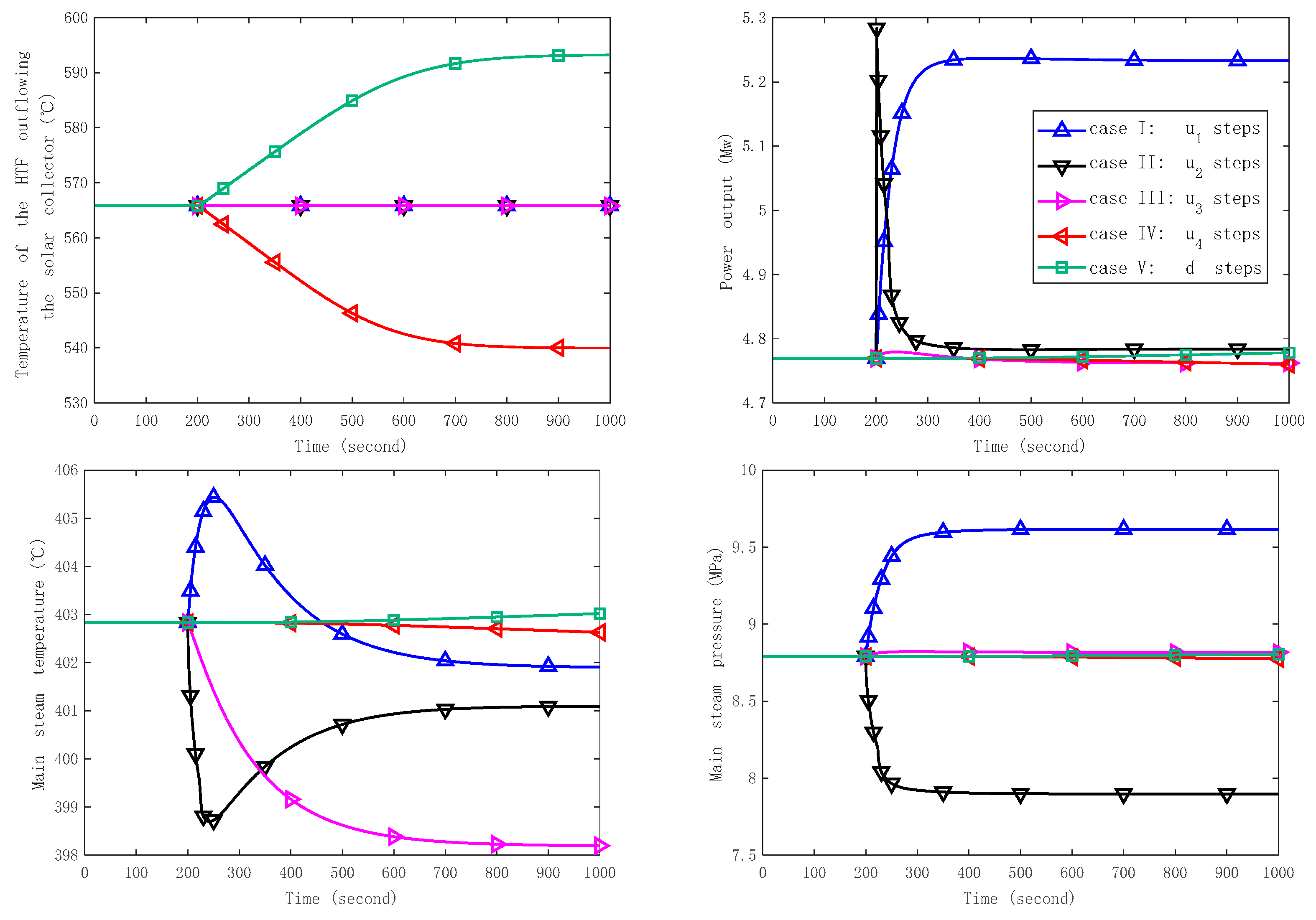
Step response simulation is carried out on the exogenous input () and manipulating variables through five cases (: the mass flowrate of the HTF outflowing from the hot tank ; : opening of the main steam valve ; : the mass flowrate of the spraying water ; : the mass flowrate of the HTF outflowing from the cold tank ).
The step increase value of the step variables are shown as follows: in case I,
steps increase from 135 kg/s to 150 kg/s; in case II,
steps increase from 80% to 90%; in case III,
steps increase from 0.8 kg/s to 1.0 kg/s; in case IV,
steps increase from 135 kg/s to 150 kg/s; and in case V,
steps increase from 1.9 kW/m
2 to 2.1 kW/m
2. In each case, there is only one signal step, and the step signal starts at 200 s. The simulation results are plotted in
Figure 3.
Case I represents the situation where the hot tank releases the stored energy to generate more electricity. The increment in the mass flowrate of the HTF outflowing from the hot tank () significantly enhances the heat transfer from the HTF to the working fluid in the Rankine cycle and produces more superheated steam. Meanwhile, the feed water mass flowrate will increase with the steam mass flowrate to maintain a constant boiler liquid level. Although the main steam temperature initially increases because of the enhanced heat transfer, it is later cooled down by the increasing feed water and finally falls below the initial value. The main steam pressure also increases drastically as more steam is generated. In this case, the settling time of the main steam pressure and power output is approximately 150 s, which is shorter than that of the main steam temperature (about 500 s).
In case II, increasing the opening of the main steam valve () causes an instant boost in the power output, which is much faster than manipulating the mass flowrate of the HTF outflowing from the hot tank (). This indicates that the turbine dynamics is faster than the steam generator and can be operated to enforce an immediate change in the power output. However, manipulating does not change the thermal energy flowing into the power generation system; therefore, the final power output almost drops to its initial value. As increases, the flow resistance of the main steam reduces rapidly, causing a significant drop in the main steam pressure with a similar setting time as that in case I (about 150 s).
In case III, the increment in the mass flowrate of spraying water (
) greatly lowers the main steam temperature, while it only has a minor influence on the main steam pressure, because the increased amount of the spraying water is very small compared to the main steam flow. Since the spraying water increases the irreversible loss and reduces the thermal efficiency, the turbine power output is slightly reduced, as shown in
Figure 3. In this case, the setting time of the main steam temperature is approximately 500 s.
Case IV shows that increasing the HTF flowing through the collector () significantly reduces the HTF temperature at the collector outlet: from 567.5 °C to 514.5 °C within 400 s. However, it has little influence on the temperature of the HTF stored in the hot tank, owing to the large heat capacity of the stored HTF. Therefore, both the temperature and the mass flowrate of the HTF flowing into the steam generator remain unchanged, demonstrating that the manipulation of almost has no influence on the steam generation side.
In case V, with the increase of direct solar irradiance incident (), the HTF temperature in the solar collector rapidly rises from 567.5 °C to 595 °C in 600 s; however, the temperature of the hot storage tank only increases by 0.4 °C in the same timescale, which indicates that the influence from the solar irradiance on the power generation side is also significantly attenuated by the storage tanks.
3.2. Process Model Identification
From the step-response analysis, we find a strong coupling effect between the manipulating variables and the controlled variables. To quantify this effect, we introduce the maximal relative deviation of the controlled variable:
where
and
are the initial value of the step variable
and the controlled variable
, respectively.
is the step increase value of
.
is the maximal deviation of
from
in the step response. All the
values are listed in
Table 2 (
: power output;
: main steam pressure;
: main steam temperature;
: HTF temperature at the collector outlet). In the same row in
Table 2, a higher value of
means that
has a relatively stronger influence on
than the other input variables.
According to the results in
Table 2, we can ignore the dynamics between the weakly interacted input variables and the controlled variables. Then, the following process model structure can be used to describe the dynamics of the CSP plant:
where
is the transfer function from the
j-th manipulating variable to the
i-th controlled variable. This model structure indicates that the original five-input–four-output control system can be decomposed into two independent control systems: a three-input–three-output power control system (
,
,
and
,
,
) and a two-input–one-output HTF temperature control system (
,
, and
). Therefore, the control of the solar collector side and the power generation side are unrelated to each other, and we can design the power tracking controller regardless of the HTF temperature control in the solar collector. Using the step-response data, the transfer function models are identified in the System Identification toolbox in MATLAB (R2017a, The MathWorks, Inc., Natick, MA, USA) and the result is presented in Equation (22):
where the terms with superscript “*” represent the initial values of the step variables. The model fitness to the step-response data is shown in
Table 3. The high fitness value indicates that the identified model captures the key dynamics of the CSP plant.
4. Power Tracking Control System Design
This section investigates the power tracking strategy of the CSP plant. The heuristic PI control with two operation modes is first developed; then, the advanced MPC strategy is studied to further improve the control performance.
4.1. Heuristic PI Control
The PI control strategy is widely used in industrial processes owing to its convenience in parameter tuning, low implementation cost, and good robustness. In practice, PI controllers are implemented in discrete form:
where
is the sample time,
is the present sample time instance,
is the last sample time instance,
is the reference signal,
is the measurement of the controlled variable,
is the controller gain, and
is the integral time constant.
Based on heuristic knowledge, the PI control strategy with two operation modes is proposed for the CSP plant, taking account of the power tracking speed and the main steam parameter fluctuations.
A. Fast power tracking mode
In FT mode, the turbine maintains the power demands and the steam generator maintains the main steam pressure. This mode gives a fast power tracking rate, because the turbine has very fast dynamics and can immediately respond to the change of the power reference signal. However, this leads to a violent manipulation on the main steam valve, which brings substantial disturbance to the main steam pressure. This disturbance cannot be well compensated, because the steam generator has a large process inertia, and cannot generate enough steam in a timely manner to maintain the main steam pressure. In this mode, the power output, the main steam pressure, and the temperature are regulated by the opening of the main steam valve, the mass flowrate of the HTF outflowing from the hot tank, and the mass flowrate of the spraying water, respectively, via three independent PI controllers.
B. Smooth operation mode
In SO mode, the turbine maintains the main steam pressure and the steam generator maintains the power demands. This mode gives a slow power tracking rate, but a smooth operation of the main steam parameters. On one hand, it is not feasible to force aggressive control action on the sluggish steam generator to accelerate the power tracking speed, because this will cause the control system to be oscillatory and even unstable. Hence, the power tracking rate will inevitably reduce. On the other hand, when the control action on the steam generator is not strong, the main steam pressure and temperature are less disturbed and can be more easily controlled by manipulating the turbine and the attemperator. In this mode, the power output, the main steam pressure, and the temperature are regulated by the mass flowrate of the HTF outflowing from the hot tank, the opening of the main steam valve, and the mass flowrate of the spraying water, respectively, via three independent PI controllers.
4.2. Model Predictive Control Strategy
MPC is an advanced control technique that employs a model to predict the future response of the plant to the manipulating variables and minimizes the error between the plant response and the reference signal. At each sample time, the MPC solves a finite horizon optimization problem yielding a finite sequence of control actions, and only the first control action in the sequence is applied to the plant. Since MPC can automatically coordinate several control loops with strong interactions, it is recommended for the control of multivariable systems.
In this section, the state-space model-based MPC is employed to enhance the power tracking performance, and the controller design consists of three steps.
A. Construction of prediction model
A state-space model that can facilitate the design of a multivariable controller is used as the prediction model:
where
,
and
are the state vector, the input vector, and the output vector at time
k, respectively.
A,
B,
C, and
D are the system matrixes. The state-space matrixes can be obtained by converting the identified transfer function model using the MATLAB command “tf2ss”.
Then, the prediction model (24) is transformed into the augmented style to impose integral action on the MPC, so that an offset-free tracking performance can be obtained in the presence of model–plant mismatch [
21]:
where
,
,
,
,
,
is the three-order unit matrix.
By stacking up Equation (25) for
steps, the prediction of future output sequences can be obtained:
, which can be expressed using
future control sequences
:
where:
Note that the future control sequence beyond
(the control horizon) is assumed to be constant, i.e.,
.
B. Estimation of immeasurable states
Since the state-space model is developed via data identification, its state vector does not have physical meanings, and cannot be measured. Therefore, it is necessary to estimate its value via a state observer on the basis of measured inputs and outputs:
where the superscript “^” means the estimated value. The observer gain
K can be calculated if the matrix H and G and a symmetric positive definite matrix
X exist, such that the following LMI (linear matrix inequality) problem is feasible [
22]:
And the observer gain is
. At each sample time, we replace the states of
in Equation (26) with the estimated states to update the prediction model.
C. Calculation of optimal control moves
The objective function of MPC is designed to achieve an optimal trade-off between the rapidity of set-point tracking and the intensity of control actions; hence, the MPC controllers can achieve good performance more easily than conventional PI controllers that cannot ensure the optimality of control actions. By minimizing the quadratic objective function with the consideration of actuator constraints, the control moves of the MPC can be calculated:
where
is the reference signal of the controlled variables,
and
are the rate constraints of the actuators, and
and
are the amplitude constraints of the actuators.
Q and
R are the adjustable weighting matrixes for the tracking error and the control actions, respectively.
4.3. Case Study
This section presents the simulation study of power tracking control. The heuristic PI tuned using the conventional Ziegler–Nichols method is compared with MPC. The sample time for the PI controller and MPC is set at 1 s. The prediction horizon and control horizon of the MPC are
and
, respectively. The weighting matrixes in MPC are given as follows:
and
. The physical constraints of the actuator are:
,
, and
. The tuning parameters of the heuristic PI are shown in
Table 4.
The simulation case is designed as follows: initially, the power reference signal (regarded as the power generation schedule) is set at 4.78 MW. At 200 s and 1000 s, it changes from 4.78 MW to 5.5 MW and to 3.0 MW, respectively. The direct solar irradiance incident on the solar collector is initially set at 1.9 kW/m
2; at 1500 s, it reduces to 1.0 kW/m
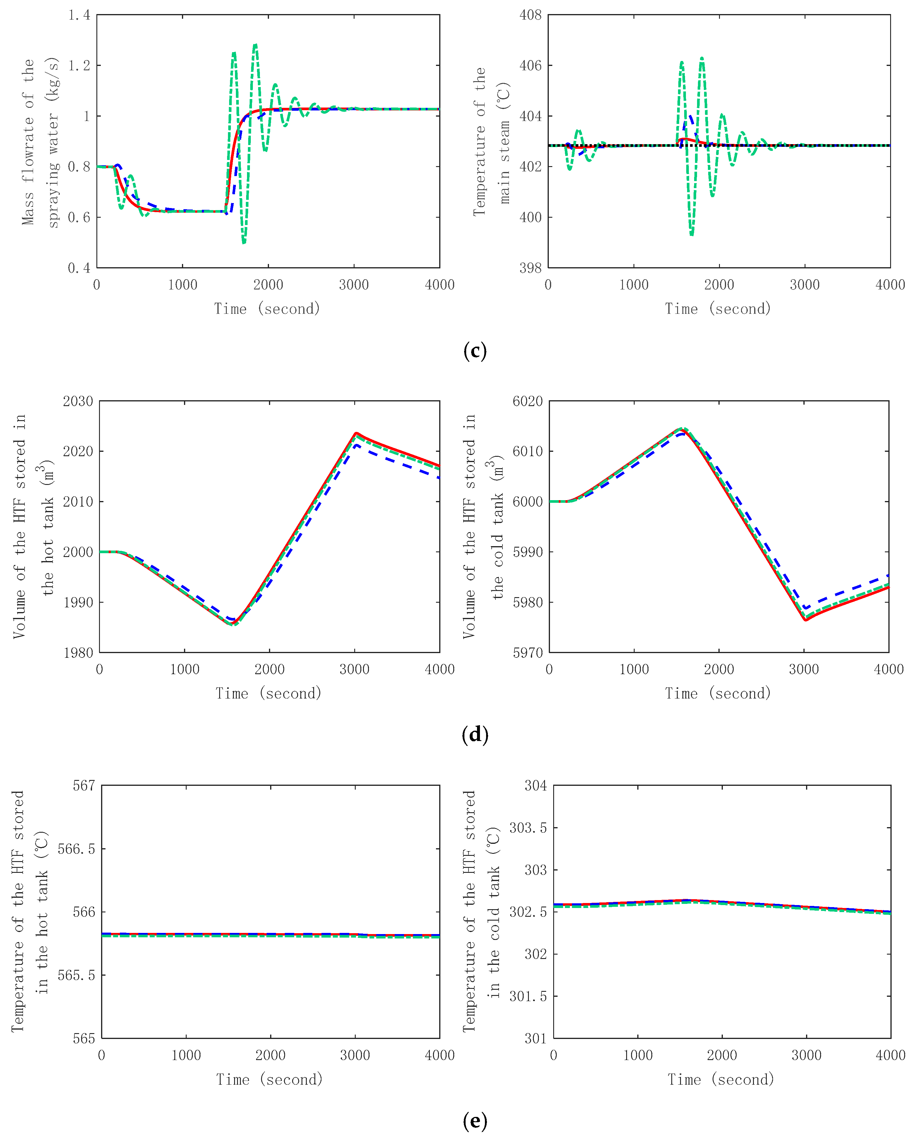
2. The reference signal of the main steam temperature and pressure are set as 402.8 °C and 8.79 MPa, respectively. The simulation results are shown in
Figure 4. Note that since the control of the HTF temperature at the collector outlet is not studied in this paper, we use a well-tuned PI controller to control it in the simulation cases. The status of the TES system is also presented to analyze the energy flow of the CSP plant.
As shown in
Figure 4a–c, the MPC has the best performance: a fast power tracking rate and the least fluctuation in main steam parameters. When the power reference signal increases/decreases, the MPC increases/decreases the mass flowrate of the HTF outflowing from the hot tank and the main steam valve opens on time, controlling the power output of the CSP plant rapidly to follow the power generation schedule, as shown in
Figure 4a. Since the MPC can anticipate the interactions between the different control loops, the change rate of the main steam valve opening and spraying the water mass flowrate is well coordinated with the change rate of the mass flowrate of the HTF from the hot tank, so that the pressure and temperature of the main steam are closely maintained to their set points.
However, the PI controllers cannot achieve a fast power tracking and a smooth operation simultaneously. In FT mode, the heuristic PI attains a similar power tracking rate to the MPC, while there are significant fluctuations in the main steam parameters. As shown in
Figure 4b, the main steam valve quickly opens to instantly generate the power required by the generation schedule. This brings significant disturbance to the steam pressure. However, unlike the MPC, the heuristic PI (FT mode) cannot predict the influence of such incoming disturbance, and it only uses the sluggish steam generator to regulate the rapidly changing pressure, which inevitably results in an untimely adjustment. Additionally, the main steam temperature is also disturbed by the frequent regulation in the main steam pressure, which results in an oscillatory transient and is difficult to be compensated by the single-looped PI.
In SO mode, the heuristic PI has a smooth transient of main steam parameters but a much lower power tracking rate (approximately 200 s slower than the PI of the FT mode and the MPC). The control moves for power tracking are quite conservative so that it does not cause substantial variations in the main steam parameters. This low-level disturbance can be timely eliminated by the PI controller. However, even with such a mild control action, the fluctuation of the main steam parameters is still more intensive than that of the MPC.
In summary, although the trend of the control actions is reasonable, the single loop-based heuristic PI does not consider the strong interactions between the multiple loops, and hence is unable to give the best control action. Additionally, owing to the past error-based mechanism, it is difficult for the PI controller to satisfy the prompt control requirement of the CSP plant with slow dynamics. Therefore, the MPC can achieve an improved performance to the heuristic PI.
Figure 4d,e, presents the status of the TES system. The temperature of the HTF in the storage tanks almost has no variation; hence, the volume of the HTF stored in the hot tank alone can be regarded as the indicator of the amount of the stored thermal energy. In the starting 200 s, the received solar energy (1.9 kW/m
2) is in perfect balance with the generated power (4.78 MW), and hence, the HTF volume in the hot tank is kept constant. Then, from 200 s to 1000 s, the power reference signal increases to 5.5 MW while the received solar energy is still equivalent to 4.78 MW. The hot tank must release the stored energy to compensate for the insufficient solar energy input, which results in a gradual reduction in the HTF volume. From 1000 s to 1500 s, the power output changes to 3 MW, which is smaller than the received solar energy (4.78 MW), and the HTF volume of the hot tank increases in order to store the excessive solar energy. After 1500 s, the direct solar irradiance incident reduces to 1.0 kW/m
2, which is insufficient to provide 3 MW power output, leading to a reduction in the HTF volume in hot tank. The results show that via manipulating the storage system, both the heuristic PI and MPC can automatically adjust the energy balance between the received solar energy, the stored thermal energy, and the power output.
5. Conclusions
The execution-level power tracking control is significant to the economic, safe, and flexible operation of the CSP plant, which is challenging and had not yet been studied in previous research.
To address this issue, this paper proposes two control strategies: heuristic PI control with two operation modes, and advanced model predictive control. Step response analysis of the CSP plant is first performed, and we find that: (1) there is a strong coupling effect between the system inputs and outputs, (2) the external disturbance (the change of solar radiation) has little influence on the power generation side, and (3) in the sense of execution-level control, the design of the power tracking controller is completely independent from the HTF temperature control at the solar collector side. Then, the performance of the heuristic PI control and MPC control are compared through simulation study. The results show the following. (1) The heuristic PI with FT mode can achieve a fast power tracking rate; however, this causes a considerable fluctuation in the main steam parameters. (2) The heuristic PI with SO mode can achieve a smooth operation of the main steam parameters; however, it has a much slower power tracking rate. (3) The MPC can well handle the strong interactions between the control loops, and hence achieves the dual task of fast power tracking and smooth operation of the main steam parameters. (4) Both the heuristic PI and MPC can automatically balance the energy flow of the CSP plant.
Within the proposed MPC control scheme, the power generation schedule from the decision-level controller can be timely tracked, which guarantees the economic operation of the CSP plant. Additionally, the main steam parameters are maintained around the designed operating range, ensuring the safe operation of the plant.
Future works on the power tracking control of the CSP plant will be extended to the widely used two-tank indirect TES system, which is even more challenging because the change of solar radiation can directly influence the power output, and it is difficult to compensate for this disturbance.
Author Contributions
Conceptualization, X.L. and Y.L.; Methodology, Y.L.; Software, X.L.; Validation, X.L.; Formal Analysis, X.L.; Investigation, X.L.; Resources, Y.L.; Data Curation, Y.L.; Writing-Original Draft Preparation, X.L.; Writing-Review & Editing, Y.L.; Supervision, Y.L.; Project Administration, Y.L.; Funding Acquisition, Y.L.
Funding
This research was funded by National Key R&D Program of China grant number [2018YFB1502904], and National Natural Science Foundation of China (NSFC) grant number [51476027], [51576041], [51506029].
Conflicts of Interest
The authors declare no conflict of interest.
Abbreviations
| A | overall area, m2 |
| Â | cross sectional area, m2 |
| C | specific heat, kJ/(kg·K) |
| H | specific enthalpy, kJ/kg |
| h | heat transfer coefficient, W/(m2·K) |
| I | direct solar irradiance incident, W/m2 |
| k | thermal conductivity, W/(m·K) |
| M | mass, kg |
| P | perimeter, m |
| PI | proportional-integral |
| p | pressure, MPa |
| Q | transferred heat, kJ |
| q | mass flowrate, kg/s |
| T | temperature, °C |
| V | volume, m3 |
| w | aperture width of the solar collector, m |
| | |
| Greek letters | |
| main steam valve opening |
| emissivity |
| efficiency |
| dynamic viscosity, Pa·s |
| density, kg/m3 |
| the Stefan-Boltzmann constant, W/(m2·K4) |
| | |
| Subscripts | |
| B | boiler |
| C | collector |
| Cond | condenser |
| cold | cold tank |
| E | economizer |
| Ex | extracted steam |
| Fw | feed water |
| G | glass envelope |
| H | heat transfer fluid (HTF) |
| HA | HTF outflowing the absorber |
| HB | HTF outflowing the boiler |
| HE | HTF outflowing the economizer |
| HSh | HTF outflowing the superheater |
| hot | hot tank |
| i | inner |
| in | inlet |
| L | liquid water |
| LA | liquid water outflowing the attemperator |
| LE | liquid water outflowing the economizer |
| MB | metal in the boiler |
| MSh | metal in the superheater |
| o | outer |
| out | outlet |
| S | steam |
| SB | steam outflowing the boiler |
| St | storage tank |
| Sh | superheater |
| Sw | saturated water |
| SSh | steam outflowing the superheater |
| T | tube |
| TA | tube in the absorber |
| TB | tube in the boiler |
| TE | tube in the economizer |
| Tu | turbine |
References
- Petrollese, M.; Cocco, D.; Cau, G.; Cogliani, E. Comparison of three different approaches for the optimization of the CSP plant scheduling. Sol. Energy 2017, 150, 463–476. [Google Scholar] [CrossRef]
- Vasallo, M.J.; Bravo, J.M. A MPC approach for optimal generation scheduling in CSP plants. Appl. Energy 2016, 165, 357–370. [Google Scholar] [CrossRef]
- Vasallo, M.J.; Bravo, J.M.; Cojocaru, E.G.; Gegúndez, M.E. Calculating the profits of an economic MPC applied to CSP plants with thermal storage system. Sol. Energy 2017, 155, 1165–1177. [Google Scholar] [CrossRef]
- Cirocco, L.R.; Belusko, M.; Bruno, F.; Boland, J. Controlling stored energy in a concentrating solar thermal power plant to maximise revenue. Renew. Power Gener. IET 2015, 9, 379–388. [Google Scholar] [CrossRef]
- Liu, M.; Tay, N.H.S.; Bell, S.; Belusko, M.; Jacob, R.; Will, G.; Saman, W.; Bruno, F. Review on concentrating solar power plants and new developments in high temperature thermal energy storage technologies. Renew. Sustain. Energy Rev. 2016, 53, 1411–1432. [Google Scholar] [CrossRef]
- Casati, E.; Casella, F.; Colonna, P. Design of CSP plants with optimally operated thermal storage. Sol. Energy 2015, 116, 371–387. [Google Scholar] [CrossRef]
- Usaola, J. Participation of CSP plants in the reserve markets: A new challenge for regulators. Energy Policy 2012, 49, 562–571. [Google Scholar] [CrossRef]
- Camacho, E.F.; Gallego, A.J. Optimal operation in solar trough plants: A case study. Sol. Energy 2013, 95, 106–117. [Google Scholar] [CrossRef]
- Franchini, G.; Barigozzi, G.; Perdichizzi, A.; Ravelli, S. Simulation and performance assessment of load-following CSP plants. In Proceedings of the 3rd Southern African Solar Energy Conference, Kruger National Park, South Africa, 11–13 May 2015. [Google Scholar]
- Cirre, C.M.; Berenguel, M.; Valenzuela, L.; Camacho, E.F. Feedback linearization control for a distributed solar collector field. Control Eng. Pract. 2007, 15, 1533–1544. [Google Scholar] [CrossRef]
- Gallego, A.J.; Camacho, E.F. Adaptative state-space model predictive control of a parabolic-trough field. Control Eng. Pract. 2012, 20, 904–911. [Google Scholar] [CrossRef]
- Alsharkawi, A.; Rossiter, J.A. Towards an improved gain scheduling predictive control strategy for a solar thermal power plant. IET Control Theory Appl. 2017, 11, 1938–1947. [Google Scholar] [CrossRef]
- Nevado Reviriego, A.; Hernández-del-Olmo, F.; Álvarez-Barcia, L. Nonlinear Adaptive Control of Heat Transfer Fluid Temperature in a Parabolic Trough Solar Power Plant. Energies 2017, 10, 1155. [Google Scholar] [CrossRef]
- Rolim, M.M.; Fraidenraich, N.; Tiba, C. Analytic modeling of a solar power plant with parabolic linear collectors. Sol. Energy 2009, 83, 126–133. [Google Scholar] [CrossRef]
- Manenti, F.; Ravaghi-Ardebili, Z. Dynamic simulation of concentrating solar power plant and two-tanks direct thermal energy storage. Energy 2013, 55, 89–97. [Google Scholar] [CrossRef]
- Caputo, A.C.; Pelagagge, P.M.; Salini, P. Heat exchanger design based on economic optimisation. Appl. Therm. Eng. 2008, 28, 1151–1159. [Google Scholar] [CrossRef]
- Åström, K.J.; Bell, R.D. Drum-boiler dynamics. Automatica 2000, 36, 363–378. [Google Scholar] [CrossRef]
- Powell, K.M.; Edgar, T.F. Modeling and control of a solar thermal power plant with thermal energy storage. Chem. Eng. Sci. 2012, 71, 138–145. [Google Scholar] [CrossRef]
- De Mello, F.P. Boiler models for system dynamic performance studies. IEEE Trans. Power Syst. 1991, 6, 66–74. [Google Scholar] [CrossRef]
- Leva, A.; Maffezzoni, C.; Benelli, G. Validation of drum boiler models through complete dynamic tests. Control Eng. Pract. 1999, 7, 11–26. [Google Scholar] [CrossRef]
- Wu, X.; Shen, J.; Li, Y.; Wang, M.; Lawal, A. Flexible operation of post-combustion solvent-based carbon capture for coal-fired power plants using multi-model predictive control: A simulation study. Fuel 2018, 220, 931–941. [Google Scholar] [CrossRef]
- Wu, X.; Wang, M.; Shen, J.; Li, Y.; Lawal, A.; Lee, K.Y. Reinforced coordinated control of coal-fired power plant retrofitted with solvent based CO2 capture using model predictive controls. Appl. Energy 2019, 238, 495–515. [Google Scholar] [CrossRef]
© 2019 by the authors. Licensee MDPI, Basel, Switzerland. This article is an open access article distributed under the terms and conditions of the Creative Commons Attribution (CC BY) license (http://creativecommons.org/licenses/by/4.0/).


