A Computationally Efficient Optimization Method for Battery Storage in Grid-connected Microgrids Based on a Power Exchanging Process

Abstract

Battery storage (BS) sizing problems for grid-connected microgrids (GCμGs) commonly use stochastic scenarios to represent uncertain natures of renewable energy and load demand in the GCμG. Though taking a large number of stochastic scenarios into consideration can deliver a relatively accurate optimal result, it can also highly deteriorate the computational efficiency of the sizing problem. To make an accuracy-efficiency trade-off, a computationally efficient optimization method to optimize the BS capacities based on the power exchanging process of the GCμG is proposed in this paper. According to the imbalanced power of the GCμG, this paper investigates the power exchanging process between the GCμG, BS and external grid. Motivated by the BS dynamics, a forward/backward sweep-based energy management scheme is proposed based on the power exchanging process. A heuristic two-level optimization model is developed with sizing BS as the upper-level problem and optimizing the operational cost of the GCμG as the lower-level problem. The lower-level problem is solved by the proposed energy management scheme and the objective function of the upper-level is minimized by the pattern search (PS) algorithm. To validate the accuracy and computational efficiency of the proposed method, the numerical results are compared with the mixed integer linear programming (MILP) method. The comparison shows that the proposed method shares similar accuracy but is much more time-efficient than the MILP method.

1. Introduction

As one of the well-recognized approaches to mitigate climate change and restructure the global energy mix, microgrids integrate various types of distributed generation sources, such as photovoltaics (PV) and wind turbines (WT), to supply local loads effectively and economically [1,2]. Microgrids can be designed as an AC type or DC type, and operate either in disconnection or connection mode with external grids [3,4,5]. In particular, grid-connected microgrids (GCμGs) are a common network structure for the industrial zones and residential communities in urban areas regarding the backbone of external grids and the urgent need for renewable energy [6,7]. A GCμG is commonly connected to the external grid via the dedicated transformer (DT) and purchases electricity based on time-of-use (TOU) prices [8]. However, due to uncertain natures of renewable energy and load demand, it is a challenging task to maintain reliability and power quality for highly-penetrated GCμGs. Storage devices, such as battery storage systems (BSs), provide a feasible way to store excessive energy produced by renewable sources and supply local loads when needed. Clearly, an optimal sizing of the BS plays a crucial part in utilizing renewable energy efficiently, satisfying load demand economically and ensuring the reliability of GCμGs.

Generally, the BS sizing problem for microgrids can be formulated as an investment decision problem combined with an energy management optimization problem [9,10,11,12]. For instance, reference [13] implements the mixed integer linear programming (MILP) method to optimize the BS capacity of microgrids with the reliability criterion being considered. Researchers use particle swarm optimization to develop the novel frequency control and demand response separately in reference [14] and reference [15] to ensure stability of microgrids, which are integrated into the BS capacity optimization model to minimize the total cost of the BS. In reference [16], the capacity of the vanadium redox battery for microgrids is optimized based on the proposed optimal scheduling analysis and cost-benefit analysis and then the optimization problem is used to solve the optimal energy management problem. A concept of mix mode energy management strategy combined three different types of operating strategies is used to determine the BS capacities for GCμGs in reference [17]. A cost-benefit analysis-based BS capacity optimization framework is proposed in reference [18] which solves the MILP method.

Since the uncertain natures of renewable energy and load demand have significant impacts on the operation of microgrids when optimizing the BS capacities, a common way to characterize these uncertain natures is generating massive stochastic scenarios by sampling or building probability distribution based on historical operational data of renewable energy and load demand [19,20,21,22]. The accuracy of the optimal results can be boosted with a large number of stochastic scenarios considered. However, increasing the number of stochastic scenarios may also lead to the boom of optimization variables. For instance, in terms of the MILP method, the number of binary variables is often used as an indicator of the computational difficulty [23]. A BS capacity optimization problem considering over hundreds of stochastic scenarios would have tens of thousands of binary variables to deal with. This condition could spend dozens of hours obtaining the optimal results, or even worse, lead to no feasible solutions due to overburdened memory usage of computing equipment. To tackle this issue, a scenario reduction technique [24] is used to reduce the number of stochastic scenarios. This technique is conducive to mitigating the efficiency issues, but it could also neglect some low-probability but high-risk scenarios and accordingly, compromise the accuracy of the optimal results.

From the model point of view, it is the energy management optimization problem that needs to consider a large number of stochastic scenarios in order to represent uncertain natures of renewable energy and load demand in microgrids. Therefore, for those algorithms adopting the similar optimization framework, the dilemma of balancing accuracy and efficiency is still an open question to be answered.

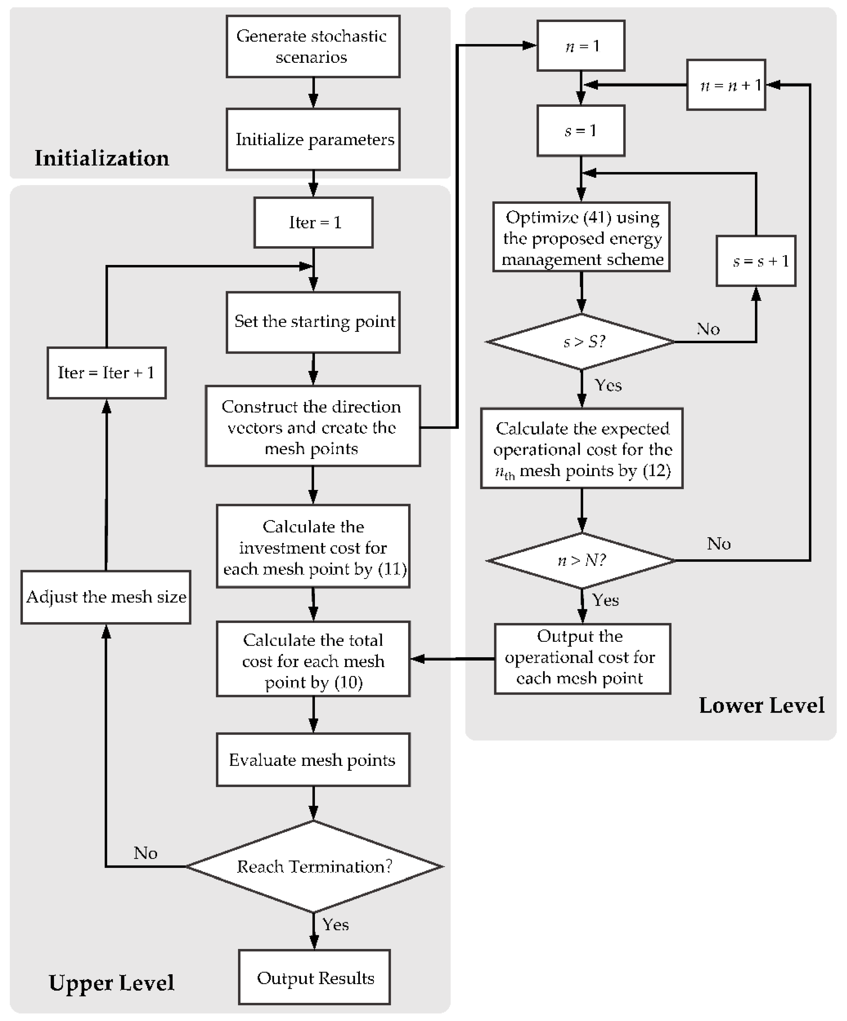
To address this problem, instead of solving the BS sizing problem directly via mathematic tools, this paper starts from the perspective of imbalanced power of renewable energy and load demand to study the power exchanging process of the GCμG with the BS and the external grid. Then, we take one of the stochastic scenarios as an example to quantify the power exchanging process with consideration of power limits of the BS and the DT. On this basis, a BS energy management scheme using the forward/backward sweep technique is proposed with consideration of the TOU prices. We solve the BS sizing problem by establishing a heuristic two-level optimization framework using the proposed energy management scheme.

The major contribution of this paper can be summarized as follows.

• Based on the imbalanced power of the GCμG, this paper investigates the power exchanging process of the GCμG with the BS and external grid. The dispatching strategies for the BS are derived from the power exchanging process analysis and then are quantified considering the power ratings of the BS and the DT.
• Motivated by the dynamics of the BS, a BS energy management scheme using the forward/backward sweep technique is proposed. This energy management scheme is able to obtain the optimal dispatching results of the BS rapidly in the context of the TOU prices.
• A heuristic two-level optimization model for sizing BS is developed using the pattern search (PS) algorithm and the proposed energy management scheme. The comparison with the mixed integer linear programming (MILP) method, which is a common approach used to address microgrid planning problems, shows that the proposed method has a similar degree of accuracy and much better computational performance.

The rest of the paper is organized as follows: Section 2 analyzes the power exchanging process of the GCμG with the BS and external grid. The optimization model for sizing the BS is summarized in Section 3. Section 4 presents the quantification of the possible dispatching strategies for the BS, followed by the forward/backward sweep-based energy management scheme proposed in Section 5. A two-level optimization framework using the proposed energy management scheme is illustrated in Section 6. Results of the numerical simulation as well as the comparison with the MILP method are presented in Section 7. Finally, Section 8 concludes the paper.

2. Power Exchanging Process of GCμG

Due to the uncertain nature of renewable sources (e.g., PV and WT) and load demand, it could easily result in power imbalance issues, assuming that a microgrid has no BSs installed or no connections with external grids. The imbalanced power caused by such an uncertain nature can be formulated as the net power of renewable sources and load demand, namely

$$\Delta P^{st}=P_{\mathrm{RE}}^{st}-P_{\mathrm{LD}}^{st}$$

(1)

where $\Delta P^{st}$ is the imbalanced power of the microgrid; $P_{\mathrm{RE}}^{st}=P_{\mathrm{PV}}^{st}+P_{\mathrm{WT}}^{st}$, representing the total power of the PV and WT; $P_{\mathrm{LD}}^{st}$ is the load demand; s and t denote the indices of stochastic scenarios and time instance, respectively.

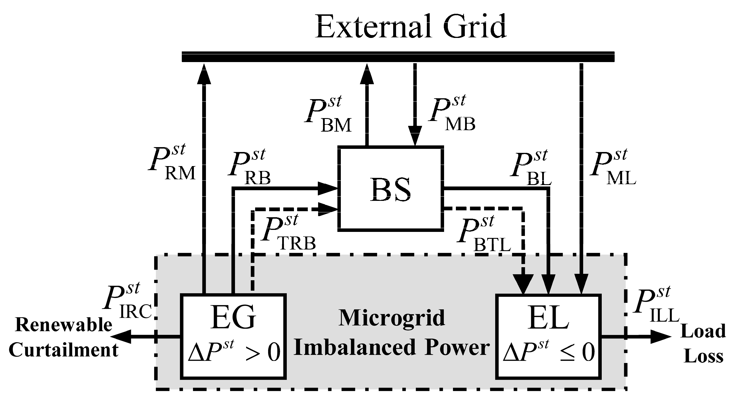
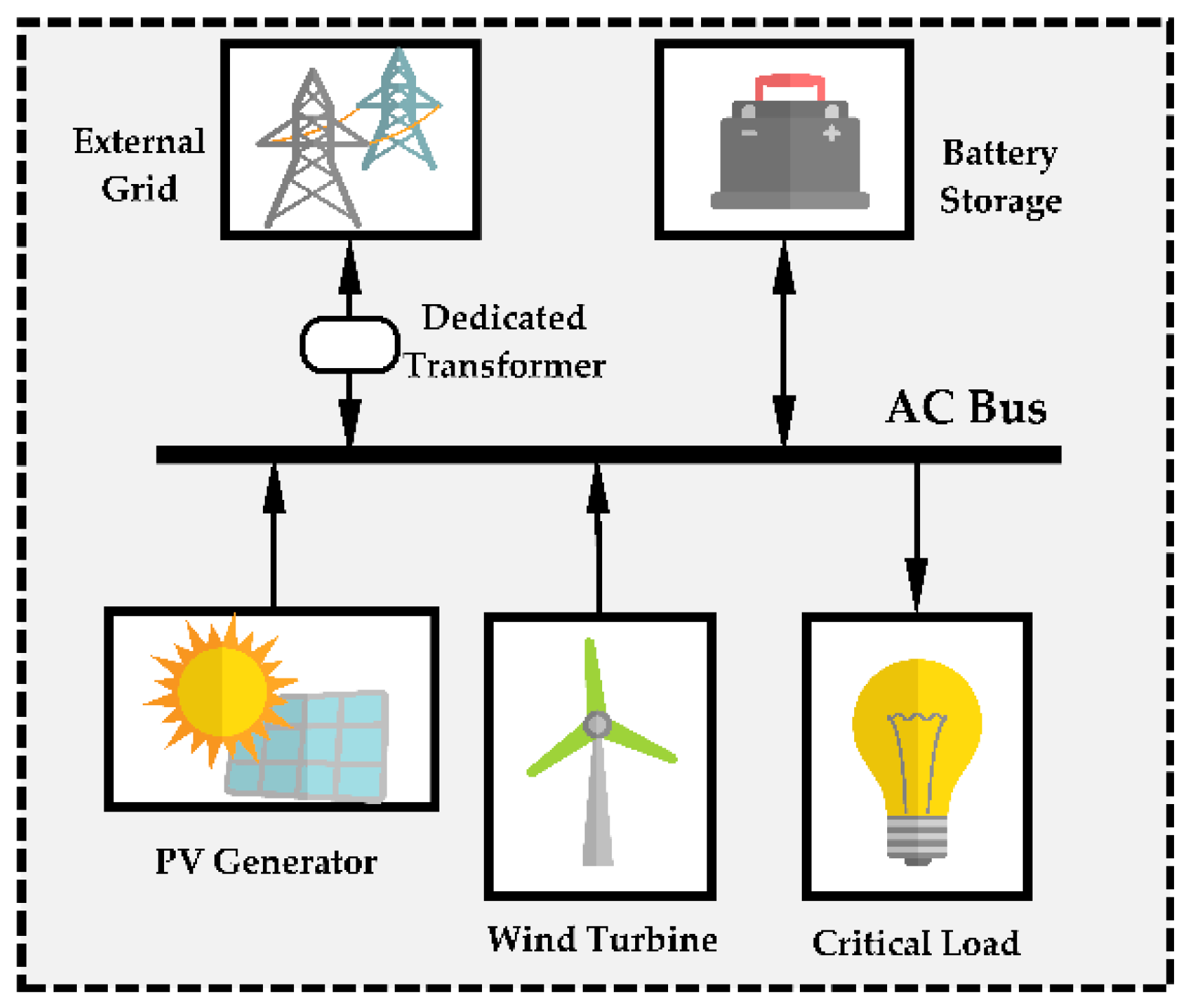
In order to completely satisfy $\Delta P^{st}$, the GCμG needs to absorb energy from or transfer energy to the BS or the external grid. The power exchanging process of the GCμG with the BS and external grid is depicted in Figure 1.

Clearly, there are three different situations that can be observed from Figure 1:

• If $\Delta P^{st}=0$, it indicates that the output of renewable sources is able to exactly meet the load demand of the GCμG and no additional power needs to be exchanged with the BS and external grid.
• If $\Delta P^{st}>0$, the imbalanced power presents a generation-like feature. It implies that there is excessive generation (EG) in the GCμG which requires the BS or the external grid to absorb. In Figure 1, $P_{\mathrm{RM}}^{st}$ denotes the part of EG that could be transferred to the external grid. Both $P_{\mathrm{RB}}^{st}$ and $P_{\mathrm{TRB}}^{st}$ denote the part of EG that could be consumed by the BS, the difference of which will be further discussed in the following sections. When the part of EG exceeds the capacities of the BS and the DT that connects the GCμG and the external grid, this part of EG, namely $P_{\mathrm{IRC}}^{st}$, will inevitably be curtailed.
• If $\Delta P^{st}\le 0$, the imbalanced power presents a load-like feature. It implies that the GCμG has excessive load (EL) that should be supplied by the BS or the external grid. In Figure 1, $P_{\mathrm{ML}}^{st}$ denotes the part of EL being supplied by the external grid. Both $P_{\mathrm{BL}}^{st}$ and $P_{\mathrm{BTL}}^{st}$ denote the part of EL being supplied by the BS, whose differences will be discussed in the following sections as well. Also, the part of EL that exceeds the capacities of the BS and the DT, namely $P_{\mathrm{ILL}}^{st}$, will inevitably be dumped.

Additionally, the BS can exchange energy with the external grid to adjust the remaining energy by operating in charging and discharging modes, i.e., $P_{\mathrm{MB}}^{st}$ and $P_{\mathrm{BM}}^{st}$.

3. Problem Formulation

3.1. Component Models of GCμG

3.1.1. Battery Storage

The BS dynamics can be formulated as

$$E_{\mathrm{B}}^{st+1}=\min ({\overline{E}}_{\mathrm{B}},\max ({\underset{\_}{E}}_{\mathrm{B}},E_{\mathrm{B}}^{st}+E_{\max }^{st}))$$

(2)

$$E_{\max }^{st}=\eta P_{\mathrm{B}}^{st}\Delta t$$

(3)

where $E_{\mathrm{B}}^{st}$ is the remaining energy stored in the BS; $P_{\mathrm{B}}^{st}$ is the available output of the BS; ${\overline{E}}_{\mathrm{B}}$ and ${\underset{\_}{E}}_{\mathrm{B}}$ are the upper bound and lower bound of the charging-discharging process and set to be 90% and 10% of the BS energy rating $E_{\mathrm{B}}$, respectively [25]; the charging-discharging efficiency $\eta =\{\begin{array}{ll}{\eta }_0,\hfill & \mathrm{charging}\hfill \\ 1/{\eta }_0,\hfill & \mathrm{discharging}\hfill \end{array}$ where ${\eta }_0=0.95$ for a sodium-sulfur (NaS) BS [26].

From Figure 1, the possible output of $P_{\mathrm{B}}^{st}$ can be given by

$$P_{\mathrm{B}}^{st}=\{\begin{array}{ll}{P}_{\mathrm{RB}}^{st}+P_{\mathrm{TRB}}^{st}+P_{\mathrm{MB}}^{st},\hfill & \mathrm{charging}\hfill \\ P_{\mathrm{BL}}^{st}+P_{\mathrm{BTL}}^{st}+P_{\mathrm{BM}}^{st},\hfill & \mathrm{discharging}\hfill \end{array}$$

(4)

Due to the power limits of the BS, $P_{\mathrm{B}}^{st}$ needs to satisfy the following constraint

$$-P_{\mathrm{B}}\le P_{\mathrm{B}}^{st}\le P_{\mathrm{B}}$$

(5)

where $P_{\mathrm{B}}$ is the BS rating power. Besides, the initial energy constraint is expressed as

$$E_{\mathrm{B}}^{s0}=E_{\mathrm{B}}^{sT}=E_{\mathrm{Bini}}$$

(6)

where $E_{\mathrm{Bini}}$ is set as 50% of $E_{\mathrm{B}}$ [27].

3.1.2. Dedicated Transformer

In Figure 1, the processes of the GCμG buying electricity from and selling electricity to the external grid can be separately formulated as

$$P_{\mathrm{Mb}}^{st}=P_{\mathrm{ML}}^{st}+P_{\mathrm{MB}}^{st}$$

(7)

$$P_{\mathrm{Ms}}^{st}=P_{\mathrm{RM}}^{st}+P_{\mathrm{BM}}^{st}$$

(8)

Since the GCμG is connected via the DT with the external grid, $P_{\mathrm{Mb}}^{st}$ and $P_{\mathrm{Ms}}^{st}$ needs to meet the power limit constraint of the DT, i.e.,

$$\{\begin{array}{l}-P_{\mathrm{Mb}}\le P_{\mathrm{Mb}}^{st}\le 0\hfill \\ 0\le P_{\mathrm{Ms}}^{st}\le P_{\mathrm{Ms}}\hfill \end{array}$$

(9)

where $P_{\mathrm{Mb}}=P_{\mathrm{DT}}$ and $P_{\mathrm{DT}}$ is the rating power of the DT; generally, $P_{\mathrm{Ms}}$ is often less than $P_{\mathrm{Mb}}$, aiming at reducing the amount of energy transferred from the GCμG to the external grid.

3.2. Objective Function

In this section, a two-level optimization framework is developed to determine the BS capacities for the GCμG.

3.2.1. Upper Level

The upper level of the BS sizing problem is solved by minimizing both the investment cost of the BS and the operational cost of the microgrid, which can be expressed as

$$\min F=C_{\mathrm{B}}+C_{\mathrm{Op}}$$

(10)

where $C_{\mathrm{B}}$ represents the investment cost of the BS and $C_{\mathrm{Op}}$ is the operational cost. Since the operational cost of the microgrid is calculated over 24 h in this paper, the one-time investment cost of the BS is required to be normalized as [28]

$$C_{\mathrm{B}}=\frac{(k_{\mathrm{B}}{\phi }_{\mathrm{B}}^{\mathrm{EC}}+{\phi }_{\mathrm{B}}^{\mathrm{MC}})E_{\mathrm{B}}+k_{\mathrm{B}}{\phi }_{\mathrm{B}}^{\mathrm{PC}}{P}_{\mathrm{B}}}{365}$$

(11)

where $k=r{(1+r)}^l/[{(1+r)}^l-1]$ and r denotes the interest rate and l is the expected lifetime of the BS. ${\phi }_{\mathrm{BS}}^{\mathrm{EC}}$, ${\phi }_{\mathrm{BS}}^{\mathrm{MC}}$ and ${\phi }_{\mathrm{BS}}^{\mathrm{PC}}$ represent the capital cost of the energy rating, maintenance and power rating of the BS.

3.2.2. Lower Level

The objective of the lower level is to minimize the operational cost of the GCμG, which is defined as the expected daily cost considering all stochastic scenarios plus the fixed charges of the two-part tariff scheme, namely

$$\min C_{\mathrm{Op}}=C_{\mathrm{DT}}+{\displaystyle \sum _{s\in S}\rho (s)C_{\mathrm{Op}}^s}$$

(12)

where $\rho (s)$ and $C_{\mathrm{Op}}^s$ denote the probability and operational cost of the sth stochastic scenario, respectively. Considering that China currently implements a two-part tariff scheme for electricity pricing, (12) consists of the fixed charges and run charges [29]. Clearly, the term ${\displaystyle \sum _{s\in S}\rho (s)C_{\mathrm{Op}}^s}$ is the run charges related to the actual energy consumed by the GCμG. The term $C_{\mathrm{DT}}$ is the fixed charges that depends on the maximum capacity of the DT the GCμG has declared to the utilities, which can be expressed as

$$C_{\mathrm{DT}}=12{\phi }_{\mathrm{DT}}{P}_{\mathrm{DT}}/365$$

(13)

where ${\phi }_{\mathrm{DT}}$ is the constant electricity price related to the declared DT capacity, which is set to 23 CNY/kW per month.

4. Quantification of Power Exchanging Process

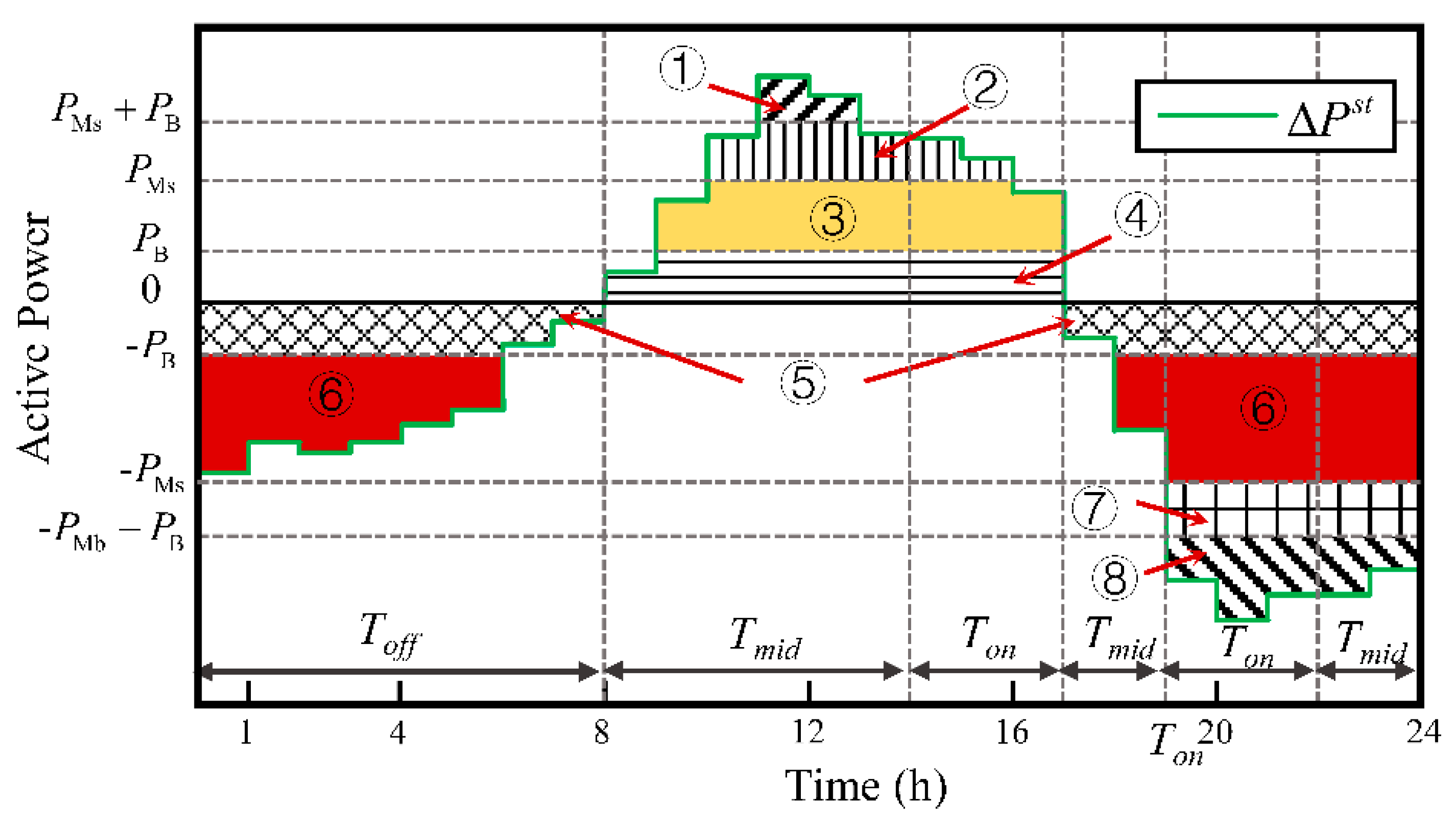
From (5) and (9), it can be noted that the power of the GCμG exchanging with the external grid and BS are limited by the power ratings of the BS and DT, namely $P_{\mathrm{B}}$, $P_{\mathrm{Ms}}$ and $P_{\mathrm{Mb}}$. Figure 2 shows the imbalanced power curve of an arbitrary stochastic scenario. If these three capacity parameters are taken into consideration in Figure 2, the imbalanced power curve can be dissected into several areas.

Due to the limited capacities of the BS and DT, the part of imbalanced power that exceeds the total sum of their capacities cannot be consumed or supplied, which refers to area ① and area ⑧ shown in Figure 2. The excessive generation in area ① and the excessive load in area ⑧ are the energy inevitably being curtailed or dumped, which can be separately calculated by

$$E_{\mathrm{IRC}}^{st}=[\Delta P^{st}-P_{M\mathrm{s}}-P_{\mathrm{B}}{]}^{+}\Delta t$$

(14)

$$E_{\mathrm{ILL}}^{st}=[\Delta P^{st}+P_{\mathrm{Mb}}+P_{\mathrm{B}}{]}^{-}\Delta t$$

(15)

where ${[\cdot ]}^{+}$ denotes the maximum value between 0 and the given value and ${[\cdot ]}^{-}$ denotes the minimum value between 0 and the given value.

Since the power in area ③ and area ⑥ is beyond the BS power rating but well within the DT power rating, these two portions of energy can be consumed or supplied by the external grid, which can be separately calculated by

$$E_{\mathrm{RM}}^{st}={[\min (\Delta P^{st},P_{\mathrm{Ms}})-P_{\mathrm{B}}]}^{+}\Delta t$$

(16)

$$E_{\mathrm{ML}}^{st}={[\max (\Delta P^{st},-P_{\mathrm{Ms}})+P_{\mathrm{B}}]}^{-}\Delta t$$

(17)

It can be noted that (14) to (17) show no relevance with the dispatching process of the BS.

In terms of the excessive generation in area ②, this part of energy is not allowed to be transferred to the external grid via the DT since it exceeds $P_{\mathrm{Ms}}$. However, the BS power rating can still cover this part of energy which, as a result, should be preferentially consumed by the BS on condition that there is sufficient energy capacity in the BS; or else, it will further increase the amount of renewable energy curtailment. This part of energy is defined as the top-prioritized renewable energy (TR). Due to the similar reasons, the excessive load in area ② cannot be supplied by the external grid but rather by the BS or else, it will further increase the amount of load loss. This part of energy is defined as the top-prioritized load demand (TL). The energy of TR and TL can be separately given by

$${\epsilon }_{\mathrm{TRB}}^{st}=min({[\Delta P^{st}-P_{M\mathrm{s}}]}^{+},P_{\mathrm{B}}){\eta }_0\Delta t$$

(18)

$${\epsilon }_{\mathrm{BTL}}^{st}={\max ({[\Delta P^{st}+P_{M\mathrm{b}}]}^{-},-P_{\mathrm{B}})\Delta t/\eta }_0$$

(19)

For clarity and analysis convenience, we use the symbol $\epsilon$ to express the energy that the BS needs to consume or supply.

The excessive generation in area ④ and excessive load in area ⑤ can be covered by both the power ratings of the BS and DT. From the perspective of economical operation, these two parts of energy should be consumed or supplied by the BS first if the BS has sufficient remaining energy. Hence, the energy in area ④ and ⑤ can be expressed as

$${\epsilon }_{\mathrm{RB}}^{st}=({[\min (\Delta P^{st},P_{\mathrm{B}})]}^{+}-P_{\mathrm{TRB}}^{st}){\eta }_0\Delta t$$

(20)

$${\epsilon }_{\mathrm{BL}}^{st}={({[\max (\Delta P^{st},-P_{\mathrm{B}})]}^{-}-P_{\mathrm{BTL}}^{st})\Delta t/\eta }_0$$

(21)

Also, the external grid can supply the BS for the charging process, which can be represented by

$${\epsilon }_{\mathrm{MB}}^{st}=\{\begin{array}{ll}{[P_{\mathrm{B}}-P_{\mathrm{TRB}}^{st}-P_{\mathrm{RB}}^{st}]}^{+}\Delta t{\eta }_0,\hfill & \Delta P^{st}>0\hfill \\ min({[\Delta P^{st}+P_{\mathrm{B}}]}^{+},P_{\mathrm{B}})\Delta t{\eta }_0,\hfill & \Delta P^{st}\le 0\hfill \end{array}$$

(22)

In (22), the condition of $\Delta P^{st}>0$ means ${\epsilon }_{\mathrm{MB}}^{st}$ should subtract the energy the microgrid supply to the BS if any whereas the condition of $\Delta P^{st}\le 0$ means ${\epsilon }_{\mathrm{MB}}^{st}$ should subtract the energy the external grid supplies to the microgrid if any.

Similarly, the BS is allowed to be discharged to send power back to the external grid, which is given by

$${\epsilon }_{\mathrm{BM}}^{st}=\{\begin{array}{ll}(P_{\mathrm{Ms}}-\min (\Delta P^{st},P_{\mathrm{Ms}}))\Delta t/{\eta }_0,\hfill & \Delta P^{st}>0\hfill \\ 0,\hfill & \Delta P^{st}\le 0\hfill \end{array}$$

(23)

(23) shows that when $\Delta P^{st}\le 0$, the BS is only permitted to supply load demand of GCμG instead of sending power to the external grid.

Additionally, when considering the electricity prices, ${\epsilon }_{\mathrm{BL}}^{st}$ plays a significant role in reducing the cost of buying electricity from the external grid while ${\epsilon }_{\mathrm{MB}}^{st}$ would increase it. In the context of the TOU electricity prices, ${\epsilon }_{\mathrm{BL}}^{st}$ and ${\epsilon }_{\mathrm{MB}}^{st}$ can be further formulated as (24) and (25), respectively, according to different time periods.

$${\epsilon }_{\mathrm{BL}n}^{st}=\{\begin{array}{c}\begin{array}{cc}{\epsilon }_{\mathrm{BL}}^{st},& t\in {\mathrm{T}}_n\end{array}\\ \begin{array}{cc}0,& t\notin {\mathrm{T}}_n\end{array}\end{array}$$

(24)

$${\epsilon }_{\mathrm{MB}n}^{st}=\{\begin{array}{c}\begin{array}{cc}{\epsilon }_{\mathrm{MB}}^{st},& t\in {\mathrm{T}}_n\end{array}\\ \begin{array}{cc}0,& t\notin {\mathrm{T}}_n\end{array}\end{array}$$

(25)

where $n\in N=\left\{off,mid,on\right\}$; off, mid and on represent the off-peak, mid-peak and on-peak periods, respectively.

5. Forward/Backward Sweeping-Based BS Energy Management Scheme

Equations (18) to (25) demonstrate the possible power exchanging processes of the BS with the GCμG and the external grid. Since the TOU electricity price has a vital impact on the operational cost of the GCμG in different time periods, Equations (18) to (25) can actually be regarded as the BS dispatching approaches with various levels of electricity price. According to the aforementioned discussions in Section 4,

Table 1. Dispatching approaches in descending order of price.

Rank Order	Dispatching Approaches	Price Level
1	${\epsilon }_{\mathrm{BTL}}^{st}$ and ${\epsilon }_{\mathrm{TRB}}^{st}$	penalty for load loss/renewable curtailment
2	${\epsilon }_{\mathrm{MB}on}^{st}$ and ${\epsilon }_{\mathrm{BL}on}^{st}$	on-peak price
3	${\epsilon }_{\mathrm{MB}mid}^{st}$ and ${\epsilon }_{\mathrm{BL}mid}^{st}$	mid-peak price
4	${\epsilon }_{\mathrm{MB}off}^{st}$ and ${\epsilon }_{\mathrm{BL}off}^{st}$	off-peak price
5	${\epsilon }_{\mathrm{RB}}^{st}$ and ${\epsilon }_{\mathrm{BM}}^{st}$	price of selling electricity

lists these dispatching approaches sorted from high to low by price.

To limit the amount of energy delivered from the BS or the GCμG to the external grid as much as possible, the price of selling electricity should be necessarily lower than buying electricity. As a whole, economically dispatching the BS can lead to a cost-effective operation of the GCμG.

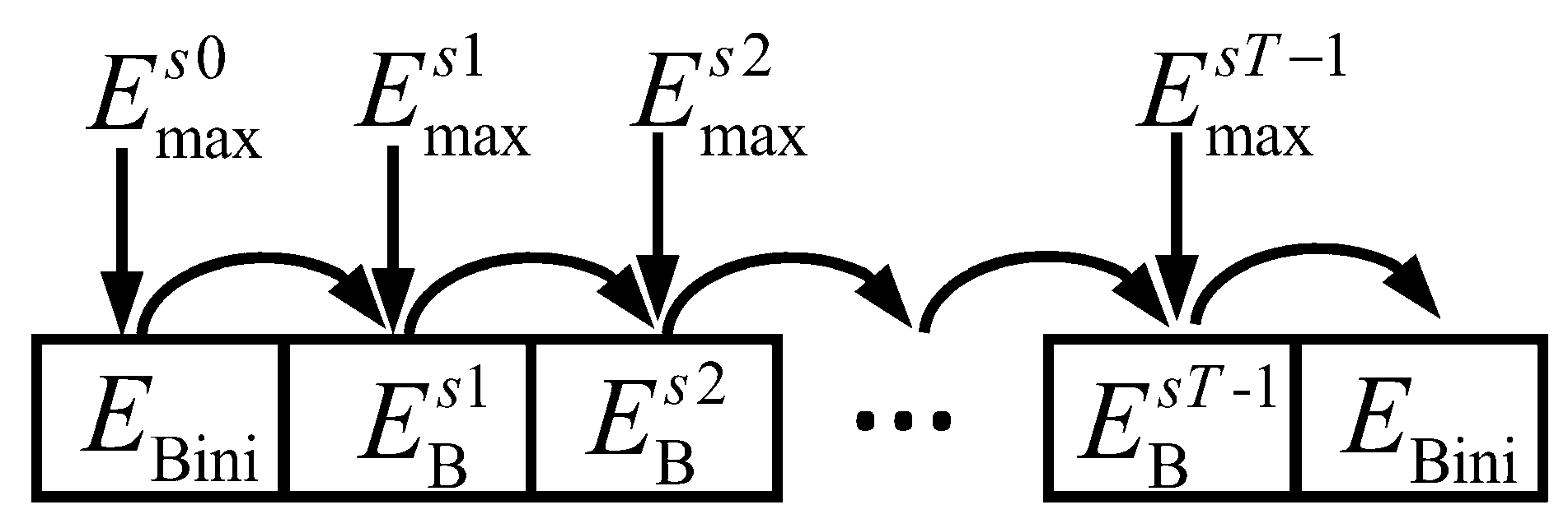
Figure 3 is the schematic of the BS dynamics based on (2), which shows that the remaining energy stored in the BS at any time instance is dependent on both the power output and the remaining energy of the BS at the previous time instance. Due to the initial energy constraint of (6), the BS remaining energy must restore itself to the same initial value either at the beginning or at the end of each day.

Motivated by the BS dynamics mentioned above, a computationally efficient energy management scheme is developed based on the forward/backward sweep technique. Before elaborating on the proposed energy management scheme, we summarize the framework of the forward/backward sweep process in Figure 4. The forward sweep is conducted to initialize the BS remaining energy to preferentially consume TR or supply TL and on-peak load while the backward sweep is used to check if the BS remaining energy at the end of the day restores to the initial values. Finally, in the correction step, it checks separately whether the GCμG handles TL and TR completely.

5.1. Forward Sweep

Ideally, the BS is required to absorb the excessive power from renewable sources and supply TL and on-peak load of the GCμG, according to the BS remaining energy capacity. In this way, the GCμG can take full advantage of renewable sources and satisfy local load demand with less dependence on the external grid and less cost of purchasing electricity. The maximum energy that the BS needs to absorb or release in this case is given by

$${\epsilon }_{\mathrm{Imax}}^{st}={\epsilon }_{\mathrm{Fw}}^{st}={\epsilon }_{\mathrm{BTL}}^{st}+{\epsilon }_{\mathrm{BL}on}^{st}+{\epsilon }_{\mathrm{TRB}}^{st}+{\epsilon }_{\mathrm{RB}}^{st}$$

(26)

Take ${\epsilon }_{\mathrm{Imax}}^{st}$ into consideration and substitute (26) into (2), then the BS dynamics can be rewritten as

$$E_{\mathrm{B}}^{st+1}=\min ({\overline{E}}_{\mathrm{B}},\max ({\underset{\_}{E}}_{\mathrm{B}},E_{\mathrm{B}}^{st}+{\epsilon }_{i\max }^{st}))$$

(27)

where i = {I, II, III}; I, II and III denote the forward sweep, backward sweep and correction step, respectively.

In the forward sweep, the remaining energy in the BS at each time instance, namely $E_{\mathrm{B}}^{st}$, can be obtained as t gradually increases to T, as depicted in Figure 5.

5.2. Backward Sweep

As stated in (6), the remaining energy stored in the BS at the end of the day should restore to the initial value to guarantee sufficient energy for the next day. However, the forward sweep does not contain this initial energy constraint and therefore, the BS remaining energy at time T calculated in the forward sweep may not be able to restore to the initial value. To measure the difference between the BS remaining energy at time T and the initial value, i.e., $E_{\mathrm{B}}^{sT}$ and $E_{\mathrm{Bini}}$, an index called remaining energy deviation is defined as follows

$${\lambda }^s=E_{\mathrm{Bini}}-E_{\mathrm{B}}^{sT}$$

(28)

If ${\lambda }^s>0$, it indicates that the BS has over-released energy to supply load demand and hence, it is necessary to increase the amount of generation to consume or decrease the amount of load demand to supply to eliminate the remaining energy deviation. In contrast, the situation when ${\lambda }^s$ is less than zero indicates the BS has overconsumed energy generated by renewable sources and hence, for the elimination of the remaining energy deviation, it should consume less renewable energy or supply more load demand. To this end, we implement the backward sweep regarding the dispatching approaches listed in Table 1, which helps to eliminate ${\lambda }^s$ rapidly and have as small an impact on the dispatching results obtained in the forward sweep as possible.

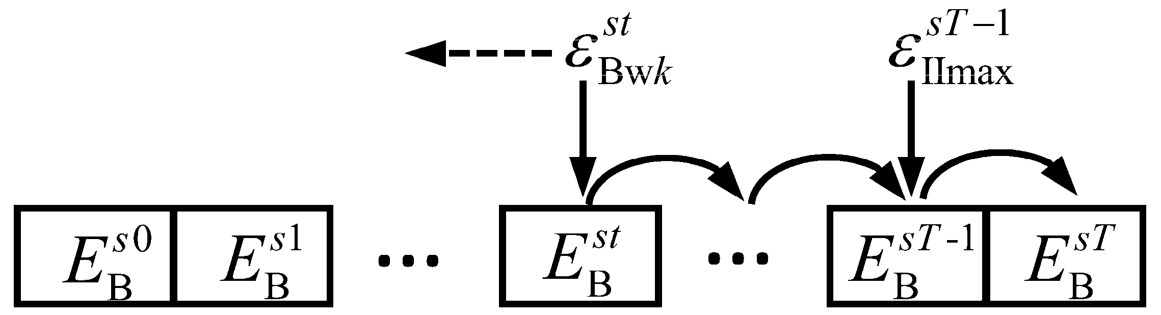
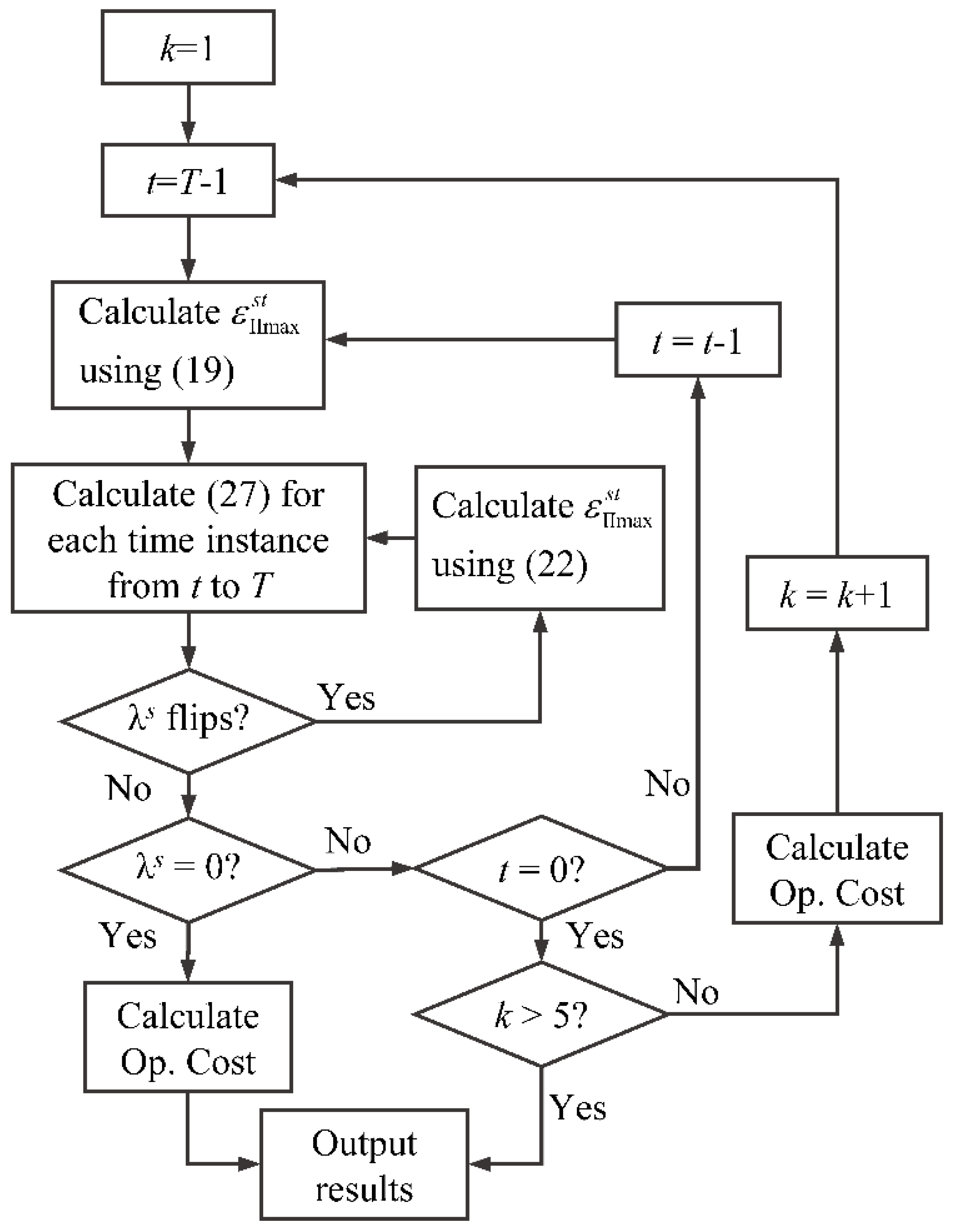
Figure 6 presents the basic process of the backward sweep where with t decreasing from T − 1 to 0, the BS remaining energy adds ${\epsilon }_{\mathrm{Bw}k}^{st}$ sequentially and then update the remaining energy from t to T. The principle to select ${\epsilon }_{\mathrm{Bw}k}^{st}$ is presented in

Table 2. Priorities of the dispatching approaches in the backward sweep.

Rank Order (k)	${\mathit{\lambda }}^{\mathit{s}}>0$		${\mathit{\lambda }}^{\mathit{s}}<0$
	${\mathit{\epsilon }}_{\mathbf{Bw}\mathit{k}}^{\mathit{s}\mathit{t}}$	${\mathit{\phi }}_{\mathbf{Bw}\mathit{k}}^{\mathit{s}\mathit{t}}$	${\mathit{\epsilon }}_{\mathbf{Bw}\mathit{k}}^{\mathit{s}\mathit{t}}$	${\mathit{\phi }}_{\mathbf{Bw}\mathit{k}}^{\mathit{s}\mathit{t}}$
1	${\epsilon }_{\mathrm{MB}off}^{st}$	${\phi }_{off}$	${\epsilon }_{\mathrm{BL}mid}^{st}$	${\phi }_{mid}$
2	${\epsilon }_{\mathrm{MB}mid}^{st}$	${\phi }_{mid}$	${\epsilon }_{\mathrm{BL}on}^{st}$	${\phi }_{on}$
3	$-{\epsilon }_{\mathrm{BL}on}^{st}$	$-{\phi }_{on}$	$-{\epsilon }_{\mathrm{RB}}^{st}$	$-{\phi }_{\mathrm{sell}}$
4	${\epsilon }_{\mathrm{MB}on}^{st}$	${\phi }_{on}$	${\epsilon }_{\mathrm{BM}}^{st}$	${\phi }_{\mathrm{sell}}$
5	$-{\epsilon }_{\mathrm{BTL}}^{st}$	$-{\phi }_{\mathrm{LL}}$	$-{\epsilon }_{\mathrm{TRB}}^{st}$	$-{\phi }_{\mathrm{RE}}$

. The maximum energy that the BS needs to absorb or release in the backward sweep is given by

$${\epsilon }_{\mathrm{IImax}}^{st}={\epsilon }_{\mathrm{Imax}}^{st}+{\epsilon }_{\mathrm{Bw}k}^{st}$$

(29)

Substitute ${\epsilon }_{\mathrm{IImax}}^{st}$ into (27) to obtain the remaining energy at t + 1 time instance and then sequentially update the remaining energy from t + 2 to T as well as calculate ${\lambda }^s$. If ${\lambda }^s$ flips, which means the value of the ${\lambda }^s$ flips from positive to negative and vice versa, (29) should be rewritten as (30) and recalculate the BS remaining energy from t + 1 to T. If not, let t = t − 1 and repeat the calculation process. If t = 0, it implies the end of the k_th backward sweep process and then, let k = k + 1 and start another backward sweep process with the ${\epsilon }_{\mathrm{Bw}k+1}^{st}$. The flowchart of the backward sweep is summarized in Figure 7. As shown in Figure 7, the maximum value of k in the back sweep is set to 5 according to Table 2.

$${\epsilon }_{\mathrm{IImax}}^{st}={\epsilon }_{\mathrm{Imax}}^{st}+{\epsilon }_{\mathrm{Bw}k}^{st}+{\lambda }^s$$

(30)

At the end of each backward sweep process or when ${\lambda }^s$ flips, the operational cost of the kth backward sweep process is given by

$$C_{\mathrm{Bw}k}^{st}=\{\begin{array}{ll}{\phi }_{\mathrm{Bw}k}^{st}{[{\epsilon }_{\mathrm{Bw}k}^{st}-\Delta E^{st}]}^{+}/{\eta }_0,\hfill & {\epsilon }_{\mathrm{Bw}k}^{st}>0\hfill \\ {\phi }_{\mathrm{Bw}k}^{st}{[{\epsilon }_{\mathrm{Bw}k}^{st}-\Delta E^{st}]}^{-}{\eta }_0,\hfill & {\epsilon }_{\mathrm{Bw}k}^{st}\le 0\hfill \end{array}$$

(31)

where $\Delta E^{st}=E_{\mathrm{B}}^{st}-E_{\mathrm{B}}^{st-1}$. Consequently, the operational cost in the backward process can be written as

$$C_{\mathrm{Bw}}^s={\displaystyle \sum _{k\in \mathrm{Bw}k}{\displaystyle \sum _{t\in T}{C}_{\mathrm{Bw}k}^{st}}}$$

(32)

5.3. Correction Step

The backward sweep regulates the power exchanging process of the BS with the external grid and the GCμG to satisfy the initial energy constraint shown in (6). However, it cannot yet ensure the GCμG to sufficiently consume the TR and supply the TL. Let the unhandled parts of the TR and TL be expressed as

$${\Gamma }_{\mathrm{TR}}^s={\displaystyle \sum _{t\in T}\Delta E_{\mathrm{TR}}^{st}}$$

(33)

$${\Gamma }_{\mathrm{TL}}^s={\displaystyle \sum _{t\in T}\Delta E_{\mathrm{TL}}^{st}}$$

(34)

where

$$\Delta E_{\mathrm{TR}}^{st}=\{\begin{array}{cc}{[{\epsilon }_{\mathrm{TRB}}^{st}-\Delta E^{st}]}^{+},& {\epsilon }_{\mathrm{TRB}}^{st}>0\\ 0,& {\epsilon }_{\mathrm{TRB}}^{st}\le 0\end{array}$$

(35)

$$\Delta E_{\mathrm{TL}}^{st}=\{\begin{array}{cc}{[\Delta E^{st}-{\epsilon }_{\mathrm{BTL}}^{st}]}^{-},& {\epsilon }_{\mathrm{BTL}}^{st}\le 0\\ 0,& {\epsilon }_{\mathrm{BTL}}^{st}>0\end{array}$$

(36)

If ${\Gamma }_{\mathrm{TR}}^s$ or ${\Gamma }_{\mathrm{TL}}^s$ is non-zero, it could further deteriorate energy curtailment or load loss issues of the GCμG. To address these problems, the BS should either consume more generation or supply less load (for the unhandled TR), or supply more load or consume less generation (for the unhandled TL). This process is defined as the correction step.

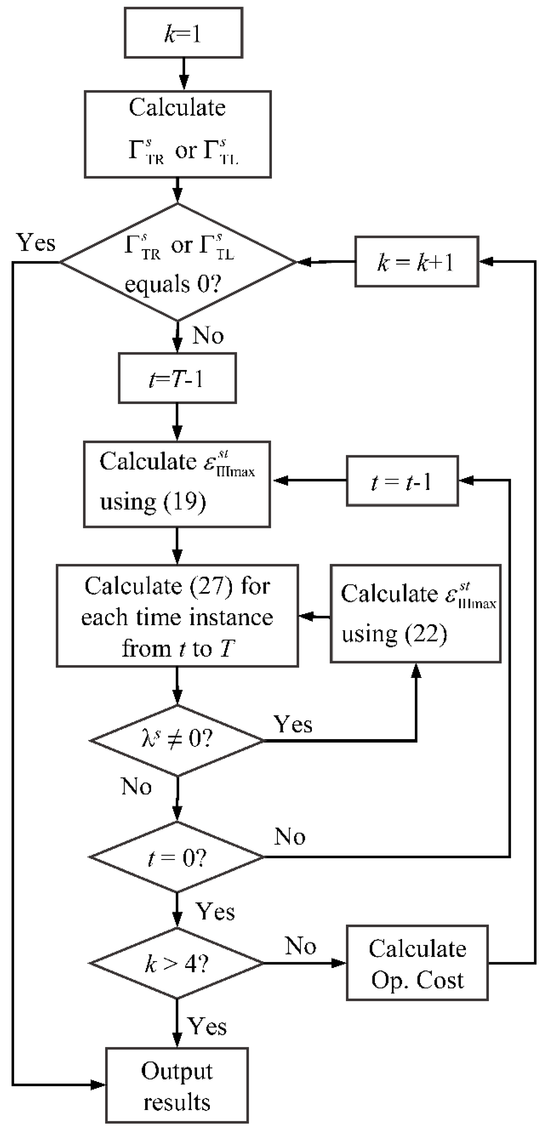
Similar to the backward sweep, the correction step calculates backward the BS remaining energy from time T to 0 with a correction of ${\epsilon }_{\mathrm{Md}k}^{st}$. The principle to select ${\epsilon }_{\mathrm{Md}k}^{st}$ is presented in

Table 3. Priorities of the dispatching approaches in the correction step.

Rank Order (k)	TR		TL
	${\mathit{\epsilon }}_{\mathbf{Md}\mathit{k}}^{\mathit{s}\mathit{t}}$	${\mathit{\phi }}_{\mathbf{Md}\mathit{k}}^{\mathit{s}\mathit{t}}$	${\mathit{\epsilon }}_{\mathbf{Md}\mathit{k}}^{\mathit{s}\mathit{t}}$	${\mathit{\phi }}_{\mathbf{Md}\mathit{k}}^{\mathit{s}\mathit{t}}$
1	${\epsilon }_{\mathrm{MB}off}^{st}$	${\phi }_{off}$	${\epsilon }_{\mathrm{BL}mid}^{st}$	${\phi }_{mid}$
2	${\epsilon }_{\mathrm{MB}mid}^{st}$	${\phi }_{mid}$	${\epsilon }_{\mathrm{BL}on}^{st}$	${\phi }_{on}$
3	$-{\epsilon }_{\mathrm{BL}on}^{st}$	$-{\phi }_{on}$	$-{\epsilon }_{\mathrm{RB}}^{st}$	$-{\phi }_{\mathrm{sell}}$
4	${\epsilon }_{\mathrm{MB}on}^{st}$	${\phi }_{on}$	${\epsilon }_{\mathrm{BM}}^{st}$	${\phi }_{\mathrm{sell}}$

. The maximum energy that the BS needs to absorb or release in the backward sweep is given by

$${\epsilon }_{\mathrm{IIImax}}^{st}={\epsilon }_{\mathrm{IImax}}^{st}+{\epsilon }_{\mathrm{Md}k}^{st}$$

(37)

Similarly, substitute ${\epsilon }_{\mathrm{IIImax}}^{st}$ into (27) to obtain the remaining energy at t + 1 time instance and then sequentially update the remaining energy from t + 2 to T as well as calculate ${\lambda }^s$. If ${\lambda }^s$ is non-zero, (37) should be rewritten as (38) and recalculate the BS remaining energy from t + 1 to T. Then let k = k + 1 and start another correction process with the ${\epsilon }_{\mathrm{Md}k+1}^{st}$. The flowchart of the correction step is summarized in Figure 8. As shown in Figure 8, the maximum value of k in the correction step is set to 4 according to Table 3.

$${\epsilon }_{\mathrm{IIImax}}^{st}={\epsilon }_{\mathrm{IImax}}^{st}+{\epsilon }_{\mathrm{Md}k}^{st}+{\lambda }^s$$

(38)

At the end of each correction process, the corresponding operational cost is calculated by

$$C_{\mathrm{Md}k}^s={\displaystyle \sum _{k\in \mathrm{Md}k}{\displaystyle \sum _{t\in T}{C}_{\mathrm{Md}k}^{st}}}$$

(39)

where

$$C_{\mathrm{Md}k}^{st}=\{\begin{array}{ll}{\phi }_{\mathrm{Md}k}^{st}{[{\epsilon }_{\mathrm{Md}k}^{st}-\Delta E^{st}]}^{+}/{\eta }_0,\hfill & {\epsilon }_{\mathrm{Md}k}^{st}>0\hfill \\ {\phi }_{\mathrm{Md}k}^{st}{[{\epsilon }_{\mathrm{Md}k}^{st}-\Delta E^{st}]}^{-}{\eta }_0,\hfill & {\epsilon }_{\mathrm{Md}k}^{st}\le 0\hfill \end{array}$$

(40)

6. Solution Algorithm

The framework of the two-level BS sizing problem for the GCμG is shown in Figure 9. The upper level aims at minimizing the total cost of the GCμG, namely (10), to obtain the optimal power and energy ratings of the BS. The PS algorithm is introduced to solve the upper level, the details of which can be found in reference [30]. The inner level adopts the proposed energy management scheme to minimize the operational cost of each stochastic scenario and returns the expected operational cost calculated using (41) to the upper level to continue the execution of the PS algorithm. The main steps of the proposed method are briefly summarized as follows.

(1)

Generate stochastic scenarios via the k-means method. Initialize the parameters of the proposed method as well as the capacities of the BS and DT.

(2)

Set the current capacities of the BS and DT as the starting point of the PS algorithm. Construct the direction vectors and create the mesh points accordingly.

(3)

Calculate the investment cost for each mesh point.

(4)

With regard to each mesh point, obtain the expected operational cost using (12) after optimizing (41) for each stochastic scenario using the proposed energy management scheme. Then, return the expected operational cost of each mesh point to the upper level.

$$C_{\mathrm{Op}}^s={\displaystyle \sum _{k\in \mathrm{Bw}k}{C}_{\mathrm{Bw}k}^s}+{\displaystyle \sum _{k\in \mathrm{Md}k}{C}_{\mathrm{Md}k}^s}+{\displaystyle \sum _{t\in T}(E_{\mathrm{IRC}}^{st}{\phi }_{\mathrm{RE}}+E_{\mathrm{ILL}}^{st}{\phi }_{\mathrm{LL}}+E_{\mathrm{RM}}^{st}{\phi }_{\mathrm{sell}})}+{\displaystyle \sum _{n\in N}{\displaystyle \sum _{t\in n}{E}_{\mathrm{ML}n}^{st}}}$$

(41)

(5)

Evaluate the mesh points based on the total cost of each mesh point. Then, update the current capacities of the BS and DT.

(6)

If none of the termination criterion is reached, adjust the mesh size and return to (2); otherwise, output the current capacities of the BS and DT as the optimal results and stop the execution.

7. Case Studies

7.1. Simulation Setup

The basic structure of the studied GCμG is shown in Figure 10, including local loads with maximum value of 500 kW and a renewable generation system composed of 250 kW PV and 750 kW WT. The parameters of the BS are listed in

Table 4. Basic parameters of the BS [26,33].

Parameters	Value
Power Rating Cost (CNY/kw h) 1	2345
Energy Rating Cost (CNY/kw)	2010
Maintenance Cost (CNY/kW/yr)	536
Charging-discharging Efficient (%)	95
Initial Remaining Energy (%)	50
Life Span	15

¹ CNY is the official unit of China’s currency and 1 USD ≈ 6.7 CNY.

and the interest rate is set to 6%. The power and energy ratings of the BS and the DT capacity declared to the utilities are the major decision variables to be optimized.

The TOU electricity price of Guangzhou city used in the numerical simulations is presented in

Table 5. The TOU electricity prices of Guangzhou city.

Types	Periods	Price
On-peak	14:00~17:00	1.4782 CNY/kW h
	19:00~22:00
Mid-peak	8:00~14:00	0.9151 CNY/kW h
	17:00~19:00
	22:00~24:00
Off-peak	0:00~8:00	0.482 CNY/kW h

. The price of selling electricity is assumed to be 0.3 CNY/kW h. Both the penalties of curtailing renewable energy and dumping loads should be set larger enough, in order to avoid renewable energy curtailment and load loss as much as possible [31]. On this basis, the penalties are set to 150 CNY/kW h.

This paper implements the proposed optimization method using MATLAB in a laptop with a Core i7-6700 CPU and 8 G memory. Additionally, (2) to (13) can also be formulated as a MILP model, which is solved via CPLEX in the same laptop and used to compare with the propose optimization method.

7.2. Results and Discussion

To validate the accuracy and the computational efficiency of the proposed method in comparison with the MILP method, we generate 200 stochastic scenarios via the k-means technique [32] using the historical data of WT, PV and load demand and conduct these two methods with the same scenarios. To further analyze the impact of the scenario number on the accuracy and the computational efficiency of the optimization problem, a scenario reduction technique in reference [24] is utilized to aggregate the generated scenarios into 30, 50, 100 and 150 scenarios.

7.2.1. Accuracy Comparison

Table 6. The optimal results calculated using the proposed method and MILP method.

Optimization Method	Number of Scenarios	PDT (kW)	EB (kW h)	PB (kW)
Proposed Method	30	415.23	62.08	26.31
	50	450.32	59.97	26.85
	100	430.12	269.57	54.28
	150	443.33	245.76	53.97
	200	443.59	245.20	54.01
MILP Method	30	412.23	60.08	24.31
	50	446.61	55.58	25.22
	100	432.47	270.03	56.41
	150	443.08	243.57	54.13
	200	443.01	243.72	53.24

lists the optimal capacities obtained by the proposed method and the MILP method. Figure 11 presents the daily total cost of the GCμG, considering different numbers of stochastic scenarios.

From the optimal capacities point of view, the optimal capacities of these two methods are nearly the same since the results obtained using the proposed method slightly differ from those obtained using the MILP model by 0.3 kW (kW h) to 4 kW (kW h). In addition, the daily total cost shown in Figure 11 also proves that the results obtained by the proposed method and the MILP method are very close. In general, the proposed method shares similar accuracies with the MILP method.

In terms of the number of stochastic scenarios, if let the case with 200 stochastic scenarios be the base case, the daily total cost and the optimal capacities of the cases with 150 and 100 stochastic scenarios have subtle differences compared with the base case. Nevertheless, these differences are still tolerable. However, as the number of stochastic scenarios continues to decrease, there are relatively large differences of the optimal results among the cases with 30 and 50 stochastic scenarios and the base case. The number of stochastic scenarios is a crucial factor that determines how well stochastic scenarios can mimic the uncertainties of the GCμG, and that is to say, more stochastic scenarios can result in better performance of the BS capacity optimization.

7.2.2. Efficiency Comparison

The computational time of the proposed method and the MILP method is summarized in

Table 7. Efficiency comparison of the proposed method with the MILP method.

Number of Stochastic Scenarios	Proposed Method	MILP Method
30	612 s	338 s
50	658 s	1251 s
100	925 s	9668 s
150	1134 s	41,377 s
200	1357 s	72,372 s

. It can be observed that the MILP method consumes 2 to 40 times as much time as the proposed method when considering a large number of stochastic scenarios. Only for those cases with a small number of stochastic scenarios, such as the case with 30 scenarios in Table 7, the MILP takes less time than the proposed method. But in general, the proposed method outperforms the MILP method in terms of computational efficiency.

As suggested by references [23,34], the number of binary variables can be used as an indicator of the computational complexity for the MILP method. In our study cases, the MILP method has around 1400 binary variables for the case with 30 scenarios and over 9600 variables for the case with 200 scenarios. It can be noted that with the number of stochastic scenarios increasing, the computational time consumed by the MILP method skyrockets. In contrast, the forward/backward sweep-based energy management strategy can optimize the operational cost of the GCμG without any binary variables. Hence, the proposed method is still time-efficient when considering 200 scenarios. To make a trade-off between accuracy and efficiency, it is an effective way to adopt the proposed method if one needs to analyze a massive stochastic scenario for BS capacity optimization problems.

7.2.3. Impact of Two-part Tariff Schemes

In this paper, we assume that the fixed charges of the GCμG depend on the DT capacity declared to the utilities. Currently, China also implement another common approach to calculate the running charges, which is proportional to the maximum load demand [24]. To study the impact of these two pricing schemes on the planning results, we conduct another comparison analysis using 200 stochastic scenarios, the results of which are listed in

Table 8. Result comparison of different two-part tariff schemes.

Type	PDT (kW)	EB (kW h)	PB (kW)	Op. Cost (CNY)	Inv. Cost (CNY)	Daily Total Cost (CNY)
DT capacity based	443.59	245.20	54.01	4180.78	148.549	4329.33
Max. load based	500	129.85	36.15	4267.23	82.86	4350.09

.

From Table 8, it can be observed that if the GCμG adopt the maximum load based tariff scheme, which means the DT capacity is set to the peak load, less capacities of the BS are required and accordingly, the investment cost decreases sharply. However, this situation also indicates the GCμG exchanges power with the external grid more frequently and hence, the operational cost as well as the total cost are larger than for the DT capacity based approach.

8. Conclusions

In this paper, we investigate the power exchanging process of the GCμG with the BS and the external grid and propose a forward/backward sweep-based energy management scheme. A heuristic two-level optimization method is established using the proposed energy management scheme and the PS algorithm to determine the optimal capacities of the BS efficiently. To validate the accuracy and computational efficiency of the proposed optimization method, the numerical simulation results are compared with those calculated by the MILP method. The result analysis and comparison show that the increasing number of stochastic scenarios can boost the accuracy of the planning results but significantly slow down the calculation process when using the MILP method, while the proposed method requires much less time to deliver relatively accurate results. Therefore, it can be concluded that the proposed method outperforms the MILP method in terms of computational efficiency and has similar accuracy. Also, the study case comparing different two-part tariff schemes demonstrates that the GCμG can operate more economically when considering the transformer capacity based scheme than when considering the maximum load based scheme.

References

1. Fathima, A.H.; Palanisamy, K. Optimization in microgrids with hybrid energy systems—A review. Renew. Sustain. Energy Rev. 2015, 45, 431–446. [Google Scholar] [CrossRef]
2. Hirsch, A.; Parag, Y.; Guerrero, J. Microgrids: A review of technologies, key drivers, and outstanding issues. Renew. Sustain. Energy Rev. 2018, 90, 402–411. [Google Scholar] [CrossRef]
3. Ton, D.T.; Smith, M.A. The US department of energy’s microgrid initiative. Electr. J. 2012, 25, 84–94. [Google Scholar] [CrossRef]
4. Chowdhury, D.; Hasan, A.S.M.K.; Khan, M.Z.R. Scalable DC microgrid architecture with phase shifted full bridge converter based power management unit. In Proceedings of the 2018 10th International Conference on Electrical and Computer Engineering (ICECE), Dhaka, Bangladesh, 20–22 December 2018; pp. 22–25. [Google Scholar]
5. Hasan, A.S.M.K.; Chowdhury, D.; Khan, M.Z.R. Scalable DC microgrid architecture with a one-way communication based control Interface. In Proceedings of the 2018 10th International Conference on Electrical and Computer Engineering (ICECE), Dhaka, Bangladesh, 20–22 December 2018; pp. 265–268. [Google Scholar]
6. Hong, Y.Y.; Chang, W.C.; Chang, Y.R. Optimal sizing of renewable energy generations in a community microgrid using Markov model. Energy 2017, 135, 68–74. [Google Scholar] [CrossRef]
7. Naderi, M.; Bahramara, S.; Khayat, Y. Optimal planning in a developing industrial microgrid with sensitive loads. Energy Rep. 2017, 3, 124–134. [Google Scholar] [CrossRef]
8. Iqbal, F.; Siddiqui, A.S. Optimal configuration analysis for a campus microgrid—A case study. Prot. Control Mod. Power Syst. 2017, 2, 23. [Google Scholar] [CrossRef]
9. Quashie, M.; Bouffard, F.; Joos, G. Business cases for isolated and grid connected microgrids: Methodology and applications. Appl. Energy 2017, 205, 105–115. [Google Scholar] [CrossRef]
10. Alsaidan, I.; Alanazi, A.; Gao, W. State-of-the-art in microgrid-integrated distributed energy storage sizing. Energies 2017, 10, 1421. [Google Scholar] [CrossRef]
11. Rigo-Mariani, R.; Sareni, B.; Roboam, X. Integrated optimal design of a smart microgrid with storage. IEEE Trans. Smart Grid 2017, 8, 1762–1770. [Google Scholar] [CrossRef]
12. Khodaei, A.; Bahramirad, S.; Shahidehpour, M. Microgrid planning under uncertainty. IEEE Trans. Power Syst. 2015, 30, 2417–2425. [Google Scholar] [CrossRef]
13. Bahramirad, S.; Reder, W.; Khodaei, A. Reliability-constrained optimal sizing of energy storage system in a microgrid. IEEE Trans. Smart Grid 2012, 3, 2056–2062. [Google Scholar] [CrossRef]
14. Kerdphol, T.; Fuji, K.; Mitani, Y.; Watanabe, M.; Qudaih, Y. Optimization of a battery energy storage system using particle swarm optimization for stand-alone microgrids. Int. J. Electr. Power Energy Syst. 2016, 81, 32–39. [Google Scholar] [CrossRef]
15. Kerdphol, T.; Qudaih, Y.; Mitani, Y. Optimum battery energy storage system using PSO considering dynamic demand response for microgrids. Int. J. Electr. Power Energy Syst. 2016, 83, 58–66. [Google Scholar] [CrossRef]
16. Nguyen, T.A.; Crow, M.L.; Elmore, A.C. Optimal sizing of a vanadium redox battery system for microgrid systems. IEEE Trans. Sustain. Energy 2015, 6, 729–737. [Google Scholar] [CrossRef]
17. Sukumar, S.; Mokhlis, H.; Mekhilef, S.; Naidu, K.; Karimi, M. Mix-mode energy management strategy and battery sizing for economic operation of grid-tied microgrid. Energy 2017, 118, 1322–1333. [Google Scholar] [CrossRef] [Green Version]
18. Chen, S.X.; Gooi, H.B.; Wang, M.Q. Sizing of energy storage for microgrids. IEEE Trans. Smart Grid 2012, 3, 142–151. [Google Scholar] [CrossRef]
19. Bhuiyan, F.A.; Yazdani, A.; Primak, S.L. Optimal sizing approach for islanded microgrids. IET Renew. Power Gener. 2014, 9, 166–175. [Google Scholar] [CrossRef]
20. Yuan, C.; Illindala, M.S.; Khalsa, A.S. Co-optimization scheme for distributed energy resource planning in community microgrids. IEEE Trans. Sustain. Energy 2017, 8, 1351–1360. [Google Scholar] [CrossRef]
21. Shang, C.; Srinivasan, D.; Reindl, T. Generation-scheduling-coupled battery sizing of stand-alone hybrid power systems. Energy 2016, 114, 671–682. [Google Scholar] [CrossRef]
22. Shadmand, M.B.; Balog, R.S. Multi-objective optimization and design of photovoltaic-wind hybrid system for community smart DC microgrid. IEEE Trans. Smart Grid 2014, 5, 2635–2643. [Google Scholar] [CrossRef]
23. Alemany, J.; Kasprzyk, L.; Magnago, F. Effects of binary variables in mixed integer linear programming based unit commitment in large-scale electricity markets. Electr. Power Syst. Res. 2018, 160, 429–438. [Google Scholar] [CrossRef]
24. Mohammadi, S.; Soleymani, S.; Mozafari, B. Scenario-based stochastic operation management of microgrid including wind, photovoltaic, micro-turbine, fuel cell and energy storage devices. Int. J. Electr. Power Energy Syst. 2014, 54, 525–535. [Google Scholar] [CrossRef]
25. Bhuiyan, F.A.; Yazdani, A.; Primak, S.L. State-of-charge (SOC)-balancing control of a battery energy storage system based on a cascade PWM converter. IEEE Trans. Power Electron. 2009, 24, 1628–1636. [Google Scholar]
26. Alsaidan, I.; Khodaei, A.; Gao, W. A comprehensive battery energy storage optimal sizing model for microgrid applications. IEEE Trans. Power Syst. 2018, 33, 3968–3980. [Google Scholar] [CrossRef]
27. Alharbi, H.; Bhattacharya, K. Stochastic optimal planning of battery energy storage systems for isolated microgrids. IEEE Trans. Sustain. Energy 2018, 9, 211–227. [Google Scholar] [CrossRef]
28. Li, P.; Xu, D.; Zhou, Z.; Lee, W.-J.; Zhao, B. Stochastic optimal operation of microgrid based on chaotic binary particle swarm optimization. IEEE Trans. Smart Grid 2016, 7, 66–73. [Google Scholar] [CrossRef]
29. Hu, X.; Xu, G.; Cheng, H.; Wang, L.; Liu, Y.; Cai, Y. Joint planning of BESS and DR for industrial consumers participating in peak-shaving. In Proceedings of the 2018 IEEE Power and Energy Society General Meeting (PESGM), Portland, OR, USA, 5–10 August 2018; pp. 1–5. [Google Scholar]
30. Arabali, A.; Ghofrani, M.; Etezadi-Amoli, M.; Fadali, M.S. Stochastic performance assessment and sizing for a hybrid power system of solar/wind/energy storage. IEEE Trans. Sustain. Energy 2014, 5, 363–371. [Google Scholar] [CrossRef]
31. Li, B.; Roche, R.; Miraoui, A. Microgrid sizing with combined evolutionary algorithm and MILP unit commitment. Appl. Energy 2017, 188, 547–562. [Google Scholar] [CrossRef]
32. Xu, D.; Chen, Z.; Li, Y. Scenario tree generation approaches using K-means and LP moment matching methods. J. Comput. Appl. Math. 2012, 236, 4561–4579. [Google Scholar] [CrossRef] [Green Version]
33. LAZARD. LAZARD’s Levelized Cost of Energy Analysis; LAZARD: New York, NY, USA, 2017; Available online: www.lazard.com/media/450337/lazard-levelized-cost-of-energy-version-110.pdf (accessed on 2 November 2017).
34. Carrion, M.; Arroyo, J.M. A computationally efficient mixed-integer linear formulation for the thermal unit commitment problem. IEEE Trans. Power Syst. 2006, 21, 1371–1378. [Google Scholar] [CrossRef]
Figure 1. Illustration of the power exchanging process of the GCμG with the BS and the external grid.
Energies 12 01512 g001
Figure 2. The imbalanced power curve of a stochastic scenario dissected by the power ratings of the BS and DT.
Energies 12 01512 g002
Figure 3. Illustration of the BS dynamics.
Energies 12 01512 g003
Figure 4. The framework of the forward/backward sweep process.
Energies 12 01512 g004
Figure 5. Illustration of the forward sweep.
Energies 12 01512 g005
Figure 6. Illustration of the backward sweep.
Energies 12 01512 g006
Figure 7. The flowchart of the backward sweep.
Energies 12 01512 g007
Figure 8. The flowchart of the correction step.
Energies 12 01512 g008
Figure 9. The flowchart of the proposed optimization method.
Energies 12 01512 g009
Figure 10. The structure of the studied GCμG.
Energies 12 01512 g010
Figure 11. The daily total cost of the GCμG considering different number of stochastic scenarios.
Energies 12 01512 g011