Uncertainty Quantification of a Coupled Model for Wind Prediction at a Wind Farm in Japan

Abstract

Reliable and accurate short-term prediction of wind speed at hub height is very important to optimize the integration of wind energy into existing electrical systems. To this end, a coupled model based on the Weather Research Forecasting (WRF) model and Open Source Field Operation and Manipulation (OpenFOAM) Computational Fluid Dynamics (CFD) model is proposed to improve the forecast of the wind fields over complex terrain regions. The proposed model has been validated with the quality-controlled observations of 15 turbine sites in a target wind farm in Japan. The numerical results show that the coupled model provides more precise forecasts compared to the WRF alone forecasts, with the overall improvements of 26%, 22% and 4% in mean error (ME), root mean square error (RMSE) and correlation coefficient (CC), respectively. As the first step to explore further improvement of the coupled system, the polynomial chaos expansion (PCE) approach is adopted to quantitatively evaluate the effects of several parameters in the coupled model. The statistics from the uncertainty quantification results show that the uncertainty in the inflow boundary conditions to the CFD model affects more dominantly the hub-height wind prediction in comparison with other parameters in the turbulence model, which suggests an effective approach to parameterize and assimilate the coupling interface of the model.

1. Introduction

The growing demand for renewable energy together with social, economical and environmental constraints leads to the currently continuous development of wind power. For the sake of integrating the wind power into an existing electrical network system, active control of the output wind power is of particular importance, which relies on the prediction of the hub-height wind for the target wind farm. To this end, numerical weather prediction (NWP) models (e.g., Weather Research and Forecasting (WRF) model), which integrate fluid dynamic cores and other parameterization packages of different physical processes, such as atmospheric boundary layer turbulent closures, radiation, moist convection physics, and other physics, have been extensively used to provide reliable predictions of low-level wind [1,2]. However, these NWP models cannot take the fine terrain features into account due to the relatively lower spatial resolution. It is addressed in Zajaczkowski et al. [3] that a typical mesoscale NWP model is not able to adequately capture the wind flow features finer than 1 km, which are usually associated with complex topography. Thus, it is necessary to couple the NWP models with other high-resolution models to revolve the local fine structures of the wind field over complex terrain regions.

Computational fluid dynamics (CFD) models, which enable capturing flow structures of small scale, are increasingly employed in simulating and predicting wind flow under complex conditions. Existing works [4,5,6] reveal that CFD models can directly simulate the dynamic effect of complex terrain on the low-level wind field, and thus provide more reliable numerical results. However, most of these studies are based on idealized and controlled boundary conditions, which are not able to provide the in situ configurations for real-case applications, especially for short-term wind forecasting where the weather condition varies significantly.

Some reports in the literature have adopted CFD models with real boundary conditions given by mesoscale models to study the flow and pollutant dispersion in built-up areas [7,8,9,10]. More recently, Temel et al. [11] proposed a new planetary boundary layer (PBL) parameterization scheme for the purpose of coupling models with different scales to simulate the complex wind flows. Though those results suggest that combining mesoscale WRF with microscale CFD model is an effective way that can be used for studying and predicting urban flow and dispersions in densely built-up areas as well as wind forecasting over complex terrains, several challenges arise meanwhile due to the relatively large differences between two kinds of models which may lead to difficulties in setting the initial/boundary condition and choosing the turbulence model for the CFD model [12,13]. In other words, there are many uncertainties involved in the coupled model which largely affect simulation results. García-Sánchez and Gorlé [13] have used an uncertainty quantification (UQ) method to quantify such uncertainties in simulating wind flow over Askervein hill region and Oklahoma city with a prescribed dominant wind direction, and show the necessity to assess quantitatively the temporal and spatial sensitivity of the model output to an uncertainty in initial/boundary condition or model parameters.

The first purpose of this paper is to develop a coupled model which consists of a mesoscale NWP model and a microscale CFD model, to improve the short-term forecasts of hub-height wind for a wind farm of interest in Japan. The CFD model adopted is the open-source package, Open Source Field Operation and Manipulation (OpenFOAM), while the WRF model is used as the mesoscale NWP model. We have evaluated the capability of the coupled forecasting system for short-term wind power forecasting, which shows its great potential as a practical forecasting system for Japan area, where the geographic features are very complex compared to other places in the world. It is recognized that uncertainties as aforementioned exist in the coupled forecasting system. Thus, our second objective is to use the polynomial chaos expansion approach to quantify the uncertainties in both initial/boundary condition and the Reynolds-averaged Navier-Stokes (RANS) turbulence model in OpenFOAM, so as to clarify the most influential factors that affect the prediction of the low-level wind.

The remainder of this study is arranged as follows. In Section 2, the data set, WRF model configuration, a brief introduction of OpenFOAM and the coupling procedure in this work are presented. The polynomial chaos expansion method used for uncertainty quantification and its implementation to the present coupled system are described in Section 3. We present and discuss the capability of the coupled model and the UQ results on some representative uncertainties in the forecasting system in Section 4, and end the paper with concluding remarks in Section 5.

2. Data and Models

2.1. GFS Data and Observations

The National Centers for Environmental Prediction (NCEP) Global Forecast System (GFS) real-time forecasts which are gridded to a horizontal resolution of 0.25 × 0.25 degree are adopted as the initial/boundary conditions to drive the high-resolution mesoscale WRF model. The observed wind data are taken from 15-site (as shown in Figure 1c) at a wind farm located in south Awaji Island, Japan. These data have been processed through a quality-controlled procedure.

2.2. Mesoscale Model

The Advanced Research WRF (ARW) model version 3.6, a limited-area mesoscale model based on a fully compressible and non-hydrostatic dynamic core, is used in this study. The domain configuration of the WRF model is the same as in our previous study [14], including a parent domain and three nested domains with horizontal resolutions of 24.0 km, 6.0 km, 1.5 km, and 0.5 km, respectively. There are 35 vertically stretched eta levels, 10 of which are within the lowest 1 km used for all domains and the top level is located at 50 hPa. The topographic data are obtained from the U.S. Geological Survey (USGS) global 30 arc-s elevation (GTOPO30) data set for all domains. The 30-hour ahead hourly predictions are carried out, starting at 6:00 p.m. UTC each day. The first 6 h are considered as the spin-up time, and only the latter 24-hour forecasts are of interest.

2.3. CFD Model

The local microscale air motion is considered as incompressible turbulent flow. We use the reduced Reynolds-averaged Navier–Stokes (RANS) equations which are time-averaged equations of flow motion, to formulate the air flow,

$$\begin{array}{cc}\hfill \hfill & \frac{\partial \overline{u_k}}{\partial x_k}=0,\hfill \end{array}$$

(1)

$$\begin{array}{cc}\hfill \hfill & \rho \overline{u_j}\frac{\partial \overline{u_i}}{\partial x_j}=-\frac{\partial \overline{p}}{\partial x_i}+\frac{\partial }{\partial x_j}\left[\mu (\frac{\partial \overline{u_i}}{\partial x_j}+\frac{\partial \overline{u_j}}{\partial x_i})\right]-\frac{\partial }{\partial x_j}\rho \overline{u_i^{{}^{\prime }}{u}_j^{{}^{\prime }}},\hfill \end{array}$$

(2)

where $(¯)$ denote the Reynolds-averaged quantity, $\mu$ is the dynamic viscosity, $\rho$ is the density of dry air and $\overline{p}$ represents the pressure. The left-hand side of Equation (2) represents the change in mean momentum of fluid element owing to the unsteadiness and convection in the mean flow. The last term in Equation (2) denotes the effect of sub-grid turbulent eddies owing to the fluctuating velocity field, which need an extra model for closure.

As a kind of turbulent viscous model, a RANS model adds the turbulent viscosity ${\mu }_t$ to the dynamic viscosity in (2). We in present work employ the widely used $k-ϵ$ model presented in [15], where the turbulent viscosity is computed by

$$\begin{array}{cc}\hfill \hfill & {\mu }_t=C_{\mu }\frac{k^2}{ϵ},\hfill \end{array}$$

(3)

where $C_{\mu }$ is a model constant, $k=\frac{1}{2}(\overline{u^{{}^{\prime }2}}+\overline{v^{{}^{\prime }2}}+\overline{w^{{}^{\prime }2}})$ stands for the turbulent kinetic energy and $ϵ$ is the dispassion rate. The value of k and $ϵ$ can be obtained using the following two equations:

$$\begin{array}{cc}\hfill \hfill & \rho \frac{\partial \left(u_{j}k\right)}{\partial x_j}={\mu }_t\frac{\partial u_i}{\partial x_j}(\frac{\partial u_i}{\partial x_j}+\frac{\partial u_j}{\partial x_i})+\frac{\partial }{\partial x_j}\left[\left(\frac{{\mu }_t}{{\sigma }_k}\right)\frac{\partial k}{\partial x_j}\right]-\rho ϵ,\hfill \end{array}$$

(4)

$$\begin{array}{cc}\hfill \hfill & \rho \frac{\partial \left(u_jϵ\right)}{\partial x_j}=C_{ϵ1}\frac{ϵ}{k}{\mu }_t\frac{\partial u_i}{\partial x_j}(\frac{\partial u_i}{\partial x_j}+\frac{\partial u_j}{\partial x_i})+\frac{\partial }{\partial x_j}\left[\left(\frac{{\mu }_t}{{\sigma }_k}\right)\frac{\partial ϵ}{\partial x_j}\right]-\rho C_{ϵ2}\frac{{ϵ}^2}{k},\hfill \end{array}$$

(5)

where $C_{ϵ1}$ and $C_{ϵ2}$ are two additional model constants, computed by

$$\begin{array}{cc}\hfill \hfill & C_{ϵ1}=C_{ϵ2}-\frac{{\kappa }^2}{\sqrt{C_{\mu }}{\sigma }_{ϵ}},\hfill \end{array}$$

(6)

where $C_{\mu }={\left(\frac{u_{*}^2}{k}\right)}^2$ and $u_{*}$ is the friction velocity. ${\sigma }_{ϵ}$ and ${\sigma }_k$ are the other two model constants. The values of these model constants are usually obtained empirically and subject to tuning to fit specific applications. Standard set values of the model constants are given in

Table 1. A set of typical coefficients of the $k-ϵ$ model. [16].

Coefficient	$\mathit{\kappa }$	${\mathit{C}}_{\mathit{\mu }}$	${\mathit{\sigma }}_{\mathit{k}}$	${\mathit{\sigma }}_{\mathit{ϵ}}$	${\mathit{C}}_{\mathit{ϵ}1}$	${\mathit{C}}_{\mathit{ϵ}2}$
Standard	0.4	0.09	1.00	1.30	1.44	1.92

. We in this paper assess the impact of the uncertainties in these empirical constants on the low-level wind structures over the target region.

In this work, we use the SimpleFoam module in OpenFOAM model (ver.5) with the above RANS model to simulate the microscale low-level wind field in the wind farm site.

2.4. Coupling WRF and OpenFOAM

The two models mentioned above have been extensively verified and validated separately as mesoscale NWP model and microscale CFD model. However, it is hard to solely use either of them to reproduce adequate numerical results for the wind flow over complex terrain for an in situ operation in a target wind farm site. It is the main reason why we intend to couple these two component models together.

In practice, the coupling is implemented by using the mesoscale WRF forecasts as the boundary conditions and the initial guess to iterate the microscale OpenFOAM model at each time step. Given the output of WRF model, SimpleFOAM was driven to reach the steady solution under the instantaneous boundary forcing of the WRF model.

Figure 1 displays the configuration of WRF and OpenFOAM domains, where the grid spacing and domain size of the WRF and OpenFOAM models are quite different. The WRF domain shown here (Figure 1a) is the inner most one among the four-nested domains as described in Section 2.2, of which the horizontal resolution is 500 × 500 m, whilst the horizontal resolution of the OpenFOAM domain (Figure 1b) is chosen as 50 m in this study, which is much finer than the WRF model. The size of the OpenFOAM domain is 12 km × 12 km, which overlaps a region of 24 × 24 cells of the WRF model. This configuration is beneficial to extract information from WRF model as initial/boundary conditions to drive the OpenFOAM model. We illustrate part of the terrain and mesh for the wind farm site of interest in Figure 1c, where the finest structured mesh cells are generated with the terrain data extracted from the Shuttle Radar Topography Mission (SRTM) data set that has a resolution of approximately 90 m (3 arc-seconds). Since OpenFOAM uses the Cartesian coordinate system, the coordinates are changed from Geographic to the UTM (Universal Transverse Mercator) coordinate based on the datum and zone of WGS 84 and 53 N, respectively.

A structured mesh with hexahedral elements is generated. The lowest surfaces of the mesh elements are fitted to the terrain surface, so as to represent the topographic features accurately. Horizontally, the total number of the mesh is 240 × 240, while 30 levels are partitioned in the vertical with an expansion ratio of 1.94. The boundary condition types used in the numerical experiment are summarized in

Table 2. The boundary condition types used for OpenFOAM model in the study.

Boundary	U	p	k	Epsilon
inlet_patch	fixedValue	zeroGradient	fixedValue	fixedValue
outlet_patch	inletOutlet	fixedValue	zeroGradient	zeroGradient
ground_patch	fixedValue	zeroGradient	kqRWallFunction	epsilonWallFunction

.

2.5. Running Mean Correction

The running mean correction method has the ability of improving the raw predictions by reducing the systematic error [17,18]. In practice, running mean errors are calculated with averaging windows varying from 1 to 30 days, and those error estimates are used to forecast and correct the subsequent predictions [18]. We choose the running mean method with the averaging window of one-day as a reference to compare the performance of the coupled model proposed in this work.

3. Uncertainty Quantification

In the coupled model discussed above, there are many uncertainties and errors in the numerical models as well as the initial/boundary conditions. Some of them affect the numerical results significantly. One of the major tasks of this work is to assess the effects of the uncertainties on the low-level wind structures quantitatively. We briefly introduce the method used in this work for uncertainty quantification.

3.1. The Polynomial Chaos Expansion Approach

In the present work, we adopt the polynomial chaos expansion (PCE) approach to quantify uncertainties in the coupled model. PCE has been widely used due to its appealing efficiency resulting from high convergence ratio of the polynomial approximation [19]. The PCE approach formulates an uncertainty using a series of orthogonal polynomial basis functions. In general, any quantity with uncertainty element $\xi$ can be written as

$$f\left(\xi \right)=\sum _{k=0}^{\infty }{\widehat{f}}_k{\varphi }_k\left(\xi \right),$$

(7)

where ${\left\{{\varphi }_k\left(\xi \right)\right\}}_{k=0}^{\infty }$ stands for the orthogonal polynomial series, and ${\widehat{f}}_k$ is the corresponding coefficient which contains the effect of the uncertainty element and is computed by

$${\widehat{f}}_k=\frac{\int f\left(\xi \right){\varphi }_k\left(\xi \right)p\left(\xi \right)d\xi }{\int {\varphi }_k{\left(\xi \right)}^{2}p\left(\xi \right)d\xi },$$

(8)

where the orthogonality of the basis function is used.

Usually, the convergence ratio of the PCE approach highly depends on the choice of polynomial series [20]. We choose the Legendre polynomial basis functions to analyze the effect of uncertainty with a uniform probability distribution in this study.

We assume that the distribution of uncertainty element $\xi$ is the uniform in $[-1,1]$, so the probability density function remains constant as

$$p\left(\xi \right)=\frac{1}{2}$$

(9)

and the denominator (8) is calculated from the characteristics of the Legendre polynomials as follows:

$$\int {\varphi }_k{\left(\xi \right)}^{2}p\left(\xi \right)d\xi =\frac{1}{2k+1}.$$

(10)

The numerator of (8) is evaluated by the stochastic collocation method described below.

3.2. Calculation of Coefficient of Polynomials: Stochastic Collocation Method

In this study, the stochastic collocation method, as a non-intrusive implementation of the PCE, is used to calculate the integral of the numerator of (8) through a numerical quadrature based on the results of deterministic simulations.

Following [21], we use the Clenshaw–Curtis quadrature instead of the Gauss–Legendre quadrature in this work for computational efficiency. The numerical quadrature is conducted with respect to the uncertainty element $\xi$. We make use of the quadrature rule to determine the quadrature points ${\xi }^{\left(i\right)}$ and the corresponding weight $w^{\left(i\right)}$ in the uncertainty space. Given a set of values of a variable or a model parameter, which includes the uncertainty element ${\xi }^{\left(i\right)}$ of interest, at the quadrature points ${\xi }^{\left(i\right)}$, we conduct the deterministic numerical simulations and get the numerical solutions $f_D\left({\xi }^{\left(i\right)}\right)$ for the physical field $f\left(\xi \right)$ with uncertainty.

The numerator of (8) is computed from the Clenshaw–Curtis quadrature,

$$\int f\left(\xi \right){\varphi }_k\left(\xi \right)p\left(\xi \right)d\xi =\sum _{i=1}^M{f}_D\left({\xi }^{\left(i\right)}\right),{\varphi }_k\left({\xi }^{\left(i\right)}\right)p\left({\xi }^{\left(i\right)}\right)w^{\left(i\right)},$$

(11)

where $f_D\left({\xi }^{\left(i\right)}\right)$ represents the numerical result from the deterministic solver at the i-th quadrature point ${\xi }^{\left(i\right)}$.

In case of $k<(M-1)/2$, the coefficient of the PCE can be exactly retrieved from the Clanshaw-Curtis quadrature. Then, we can express the PCE by a truncated model as

$$\tilde{f}\left(\xi \right)=\sum _{k=0}^{(M-1)/2}{\widehat{f}}_k{\varphi }_k\left(\xi \right).$$

(12)

The convergence of this truncated PCE to the stochastic result with the errors of aliasing and numerical quadrature can be proved [19].

3.3. Statistics Using Polynomial Chaos Expansion

Once the coefficients of the PCE are determined, the statistical properties can be directly computed from the truncated PCE model (12). For example, the mean and variance can be easily obtained as follows:

$$E\left[\tilde{f}\left(\xi \right)\right]={\widehat{f}}_0,$$

(13)

$$V\left[\tilde{f}\left(\xi \right)\right]=\sum _{k=1}^{(M-1)/2}\frac{1}{2k+1}{\widehat{f}}_k^2.$$

(14)

The standard deviation (STD) is calculated as a positive root of the variance. The cumulative density function ${\mathrm{CDF}}_{\widehat{f}}$ of value $\widehat{f}$ is calculated as the integration of $p\left(\xi \right)$ over the ranges $\mathsf{\Xi }:\tilde{f}\left(\xi \right)<\widehat{f}$ as follows:

$${\mathrm{CDF}}_{\widehat{f}}={\int }_{\mathsf{\Xi }:\tilde{f}\left(\xi \right)<\widehat{f}}p\left(\xi \right)d\xi ,$$

(15)

which is computed by numerical quadrature. CDF reflects to some extent the nonlinearity in the response of the system to uncertainty $\xi$, as discussed in Section 4.3.

3.4. Experiment Design

Although coupling mesoscale WRF and microscale CFD model can improve wind forecasts over a complex region, the performance of this coupled model includes several uncertainty sources which significantly affect the forecasting results, such as the uncertainties in the lateral coupling boundary condition, the turbulent model, and the land surface parameterization, among others.

In this study, we focus on the uncertainties in inlet boundary conditions and the RANS turbulence model ($k-ϵ$) in the CFD module.

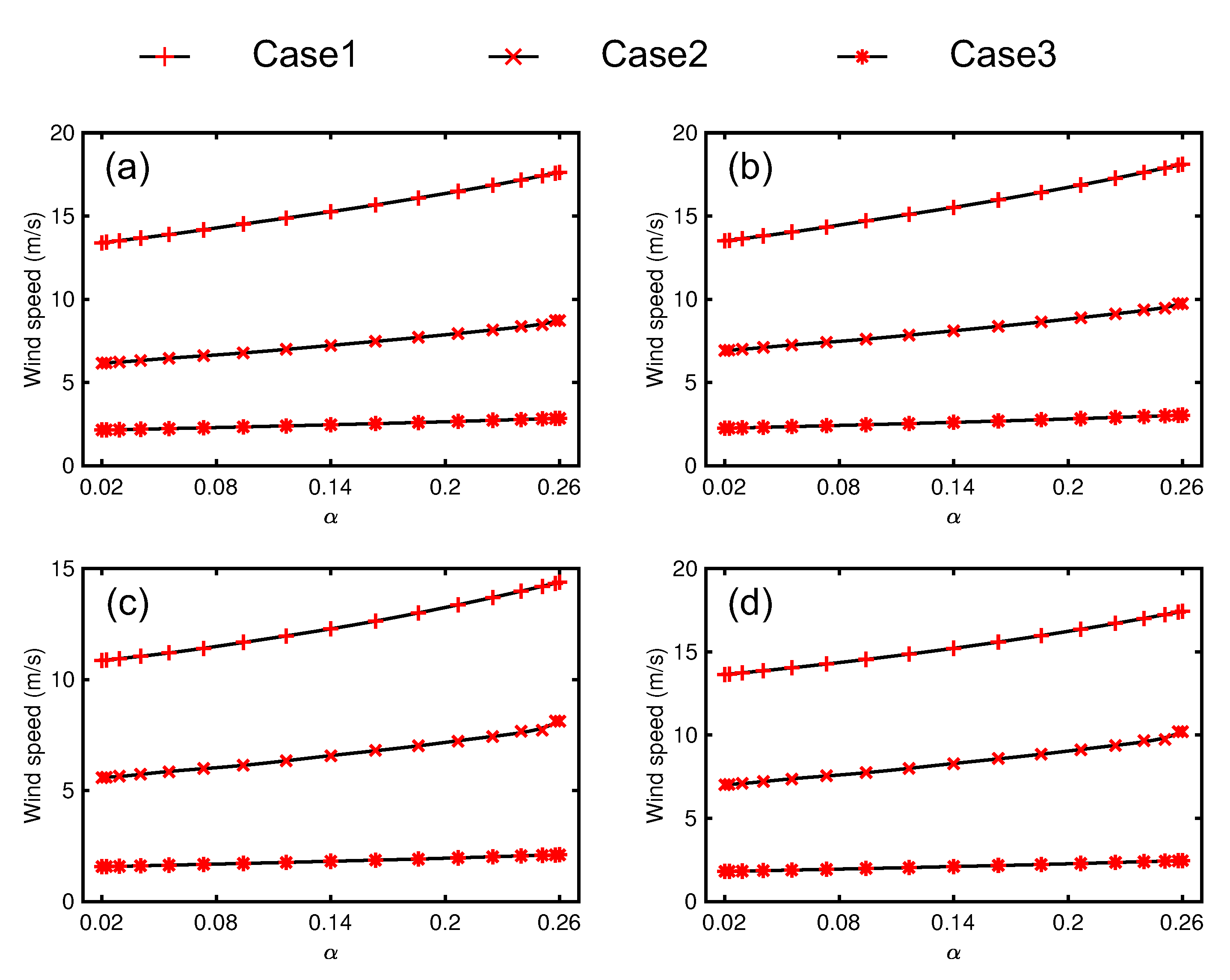
• Uncertainty in the inlet boundary condition
  The wind flow inlet boundary condition, which usually has the form of standard neutral surface layer profile [22], can significantly influence the output of a CFD model. Such a profile can be specified using the wind shear exponent $\alpha$ with the wind velocity at a reference level [1],

  $$U\left(z\right)=U_{ref}{\left(\frac{z}{z_{ref}}\right)}^{\alpha },$$

  (16)

  where $U\left(z\right)$ and $U_{ref}$ are the wind velocities at height z and reference level $z_{ref}$, respectively. The empirically estimated value of $\alpha$ is approximately 0.14 over smooth terrains [1], which however needs further tuning when applied to complex terrain conditions. Thus, we choose the shear exponent $\alpha$ as an uncertain parameter to quantify the impact of the uncertainty in the inlet boundary condition on the numerical results of the low-level flow field. We analyzed the statistics from a set of deterministic CFD simulations with different values of $\alpha$. For the sake of investigating the sensitivity of $\alpha$, a broad range varying according to a uniform distribution in the range from 0.02 (very smooth surface) to 0.26 (suburban) [23] is employed in this study.
• Uncertainties in turbulence model parameters
  We also quantified the impact of the uncertainty of the empirical parameters in the turbulence model as described in Table 1 on the wind flow forecasting at the target wind farm over complex terrain conditions.
  We set the uncertainty of each parameter as a uniform distribution with bounded values shown in

  Table 3. Admissible range of the parameters in $k-ϵ$ turbulence model.

  Parameter	Low Bound	Upper Bound
  $C_{ϵ2}$	1.248	2.88
  $C_{\mu }$	0.054	0.135
  ${\sigma }_k$	0.6	1.5
  ${\sigma }_{ϵ}$	0.78	1.95

  . The variation range of each parameter is determined by the physical and computational admissible bounds with respect to the standard values as discussed in [24].

4. Results and Discussion

In this section, we first evaluate the capability of the coupled system by simulating an in situ case. The numerical results of the prediction of the coupled model are validated with the nacelle wind observations at each wind turbine site over an 8-day period. We then quantify the impact of the uncertainties in both the parameters in the turbulence model and the inlet boundary conditions which are extracted from the mesoscale WRF model and serves the key in the coupled model.

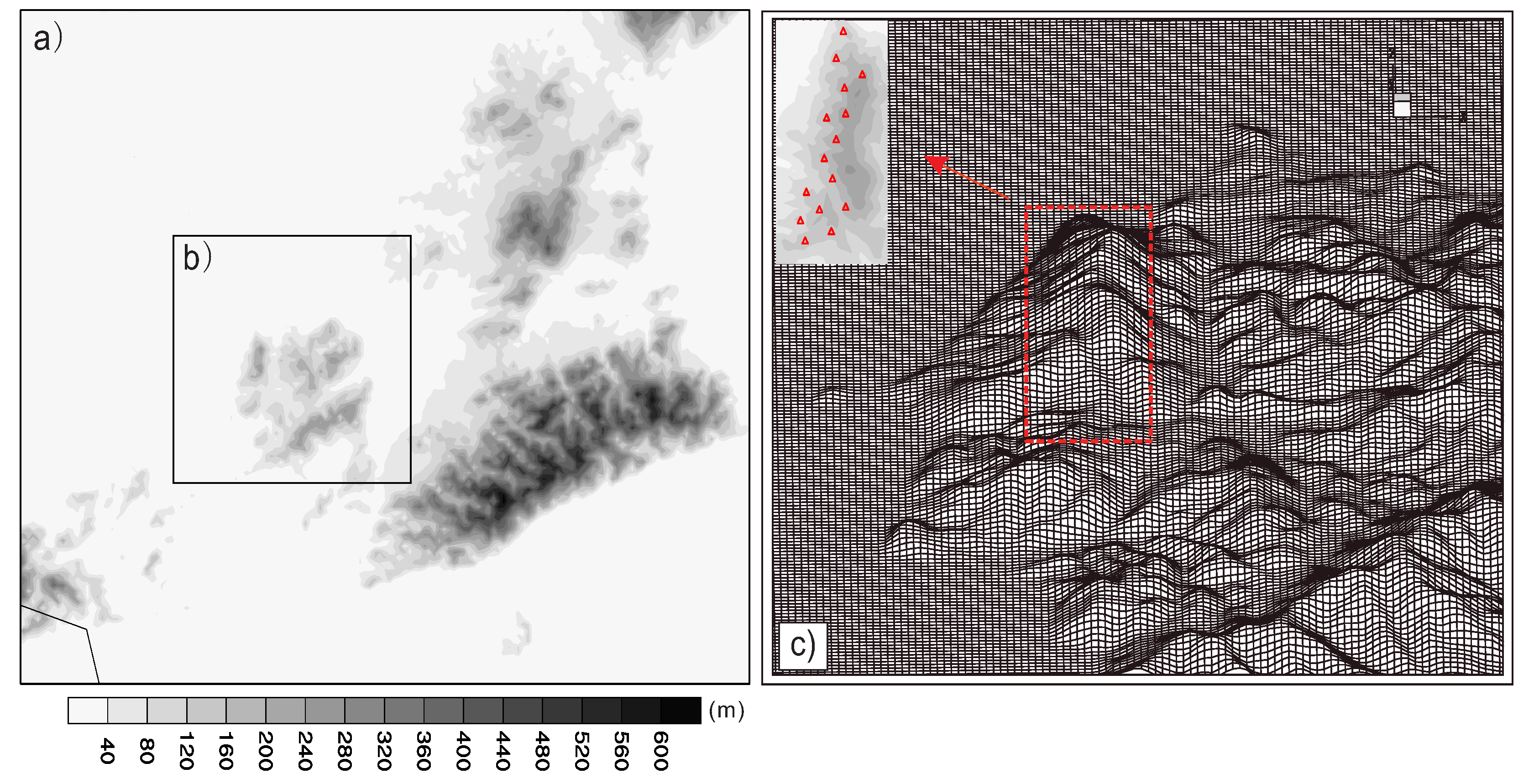
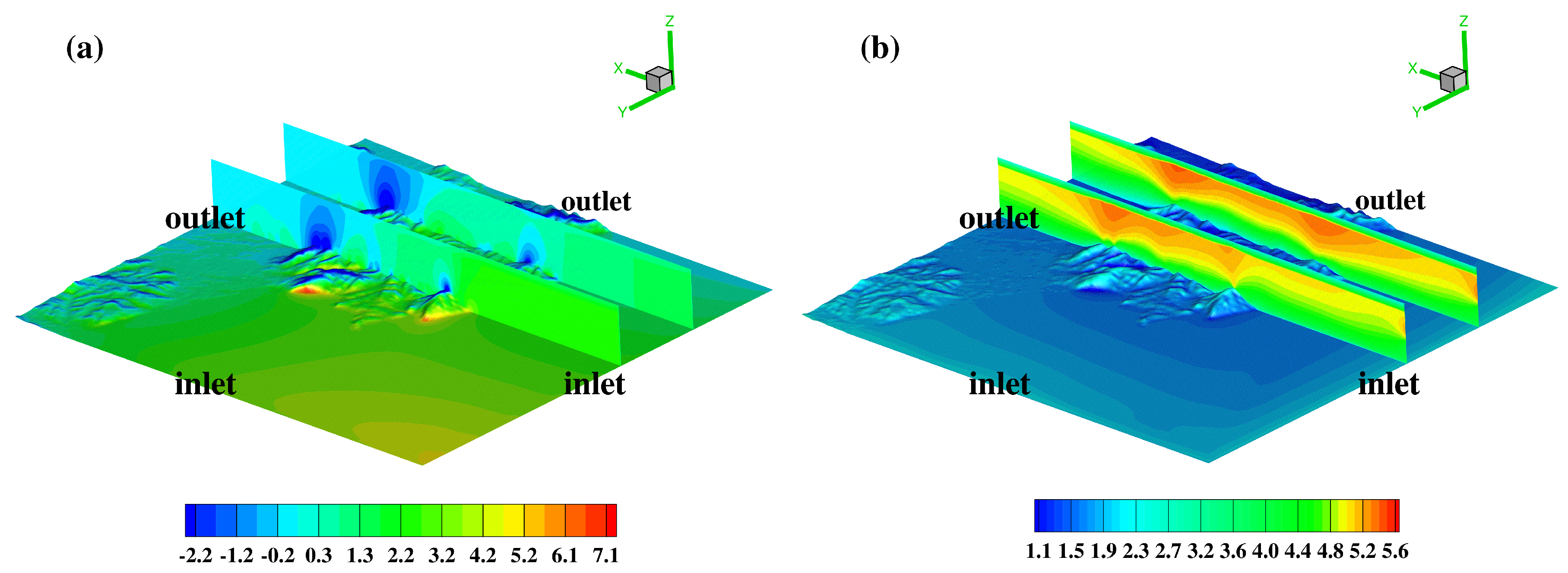
4.1. The Flow Field under Dynamic Forcing of Topography

An in situ case starting from 12:00 a.m. UTC, 1 October 2013, has been used to validate the performance of the coupled forecasting system for simulating low-level wind flow over complex terrain. As the prevailing wind is northwest, the inlet and outlet boundary conditions are set as in Figure 2. The inlet boundary condition is the output from the mesoscale WRF model. The SimpleFoam module in the OpenFOAM package with the $k-ϵ$ turbulence model is used to generate a steady flow field. Throughout all this study, we assume that the wind flow reaches a steady state when all the residuals of $U_x$, $U_y$, $U_z$ and k are smaller than ${10}^{-3}$, while the residual of p should be smaller than ${10}^{-2}$.

Figure 2a,b show the simulation results of pressure and wind speed, respectively. The distribution of the pressure is reasonably reproduced, where the dynamic forcing of the topography results in low pressure near the top of the hills and high pressure in the upwind side of the hills. The pressure fields sliced on the two vertical cross sections in $x-z$ plane in Figure 2a demonstrate that the coupled model is able to simulate the fine 3D flow structures over complex terrain. From Figure 2b, it is observed that the wind velocity over the hills is significantly accelerated and reaches the maximum around the top of the hills, while decreased on the lee side of the hills. In addition, we have also examined the turbulence kinetic energy (TKE) and found that TKE is greatly enhanced over the hills and decays out gradually in the downstream direction, which is in agreement with the theoretical observational results.

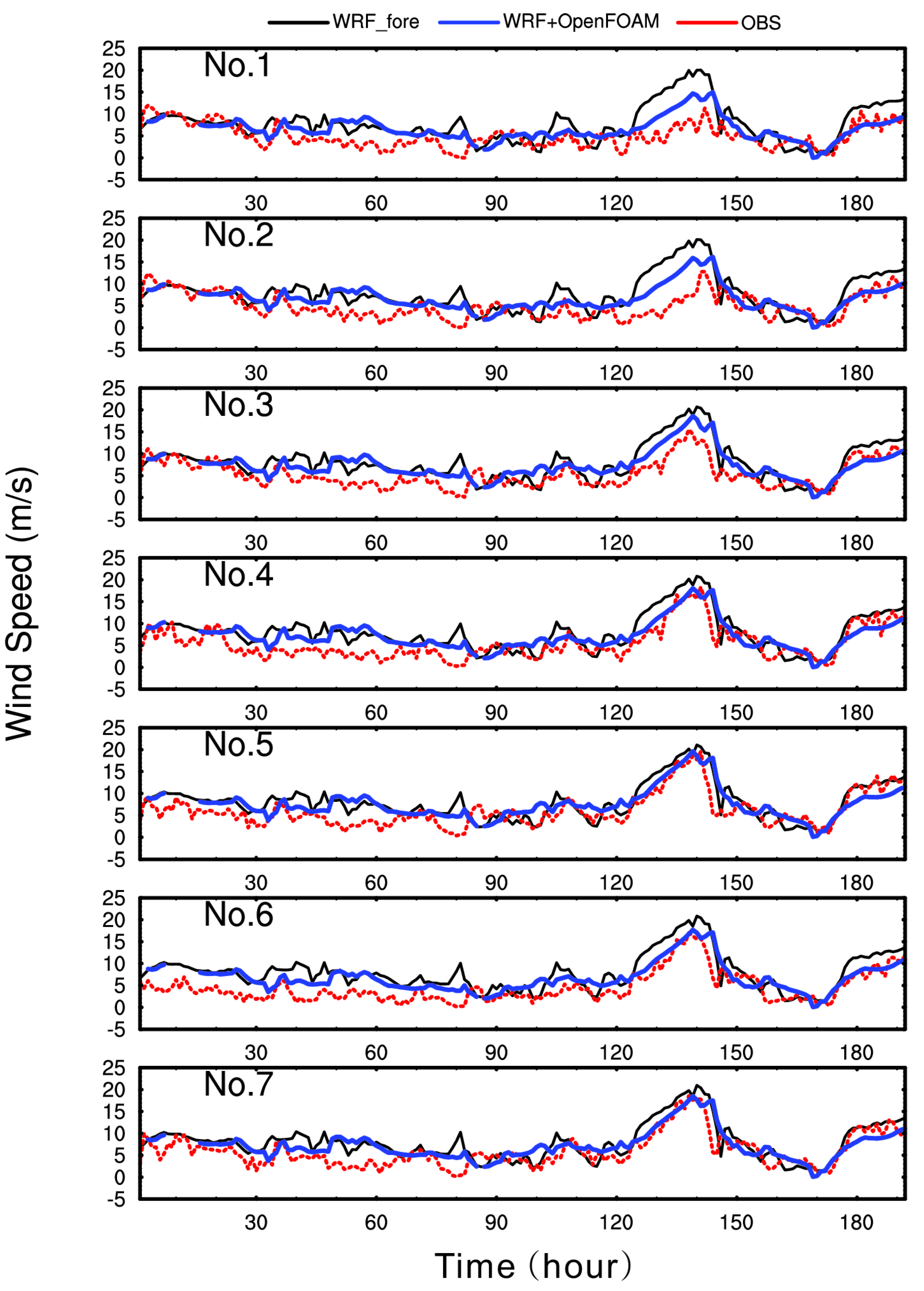
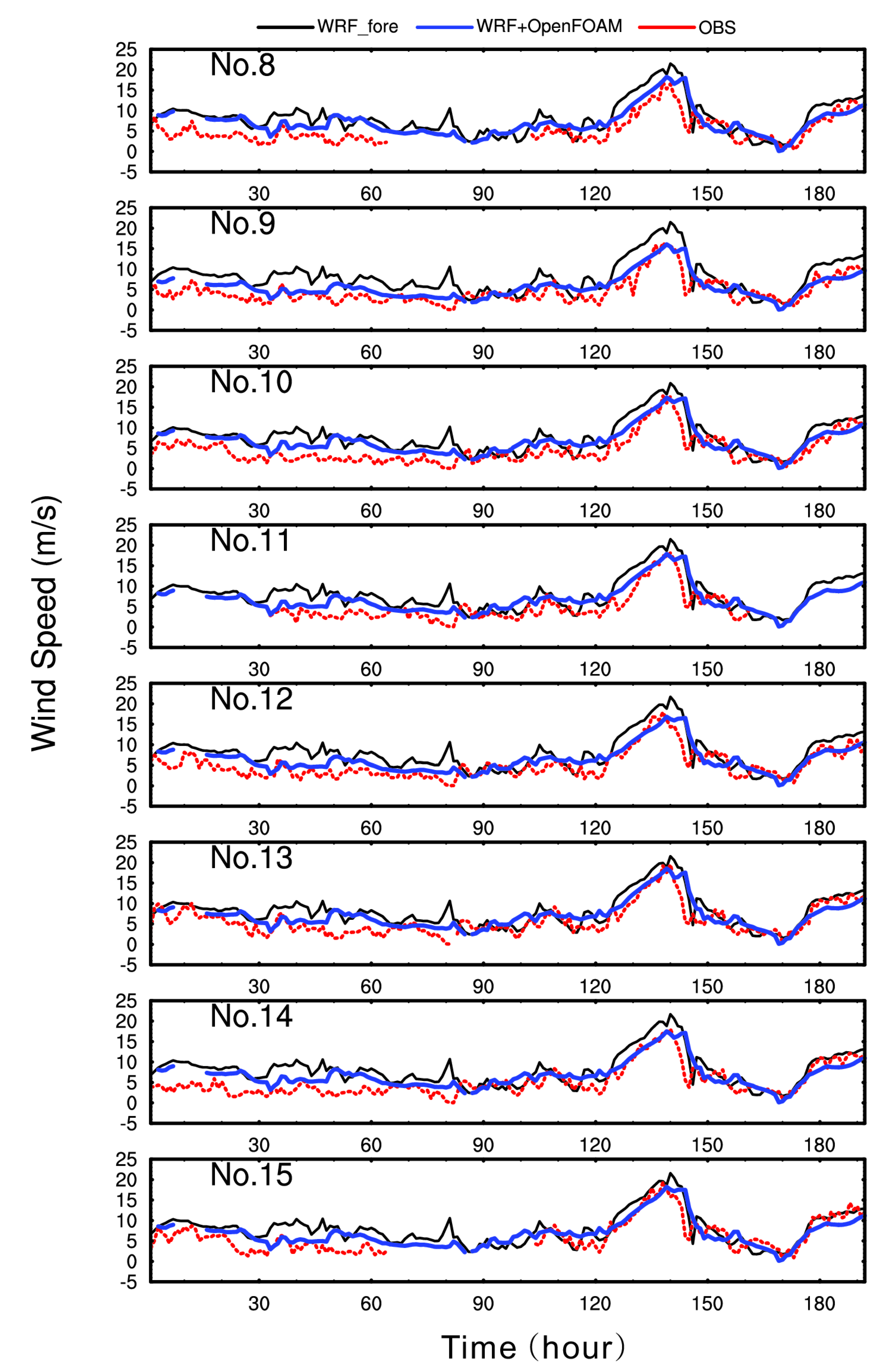
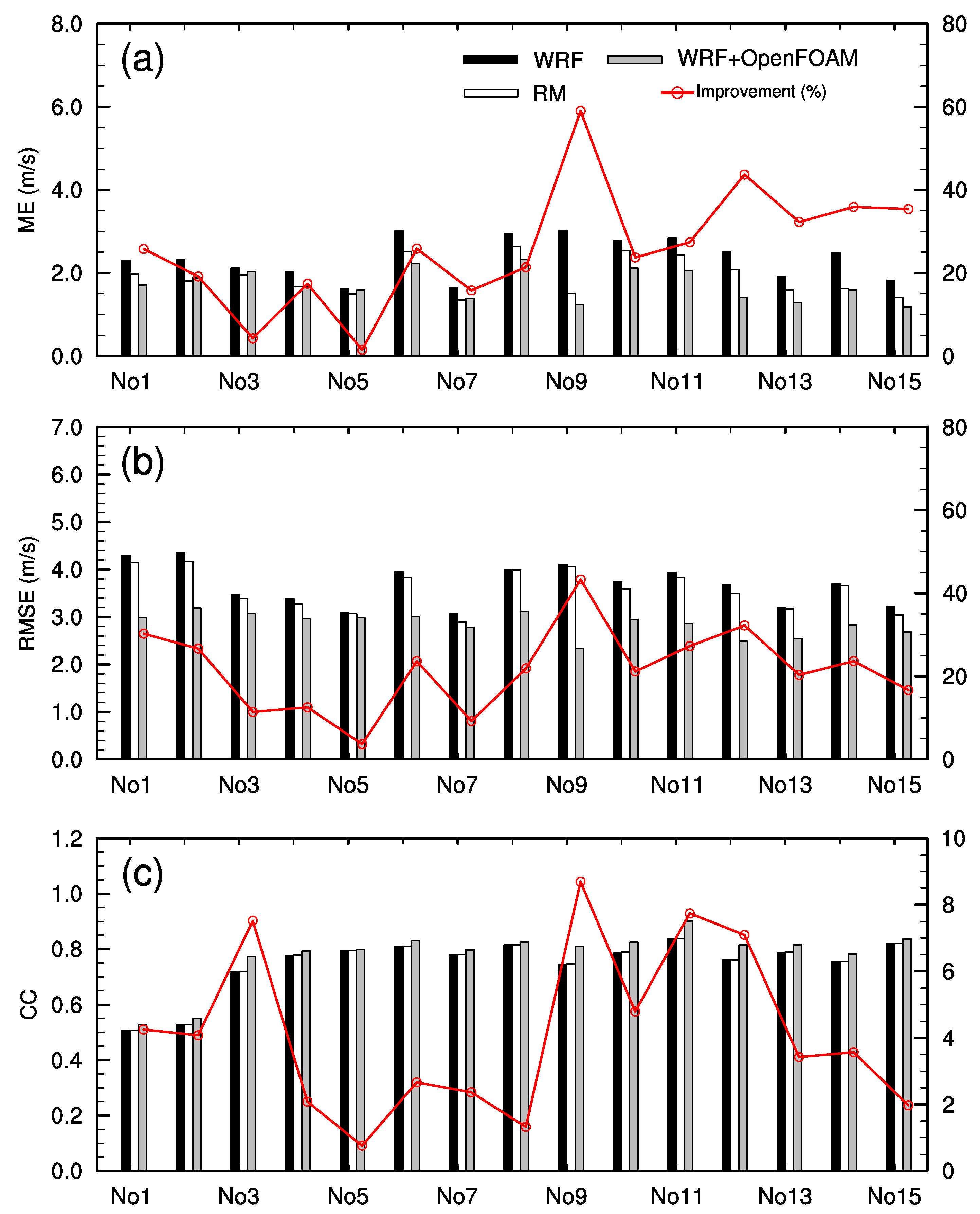
4.2. Validation of the Coupled Model for Wind Prediction

It has been demonstrated in the above section that the coupled system with the direct CFD simulation of topographic forcing the wind flow over the complex terrain can be well resolved. We extensively carried out 192 cases using the coupled model to predict the wind fields of a one-hour interval from 00:00 UTC 2 October to 23:00 UTC 9 October 2013. It is worthwhile to note that the wind directions from WRF-alone model for these cases are different. The inlet and outlet patches are determined by the prevail wind direction at level of 400-m. The forecasting results for 15 turbine sites are compared with the corresponding nacelle wind observations separately. In order to evaluate the effectiveness of the coupled forecasting system, we also include the numerical results from the forecasting system solely based on the mesoscale WRF model for comparison at some specific turbine sites of the target wind farm.

The comparisons of the wind speed predictions for all 15 wind turbine sites during the period of 00:00 UTC 2 October to 23:00 UTC 9 October 2013 are shown in Figure 3 and Figure 4, where forecasts of both the WRF model (denoted by “WRF_fore”) and the coupled model (denoted by “WRF+OpenFOAM”) are plotted against the nacelle observations (denoted by “OBS”). It is found that although the accuracy of forecasts varies among the turbines and over different periods of time, both the WRF-alone forecasts and the WRF/OpenFOAM coupled forecasts can reproduce the overall wind speed variations reasonably well for all 15 turbines. It is also observed that the coupled WRF/OpenFOAM model can significantly improve the forecasting skill, particularly for the period from 120 to 150. In spite of different extents for different turbines and different periods of time, the coupled model shows appealing prediction capability in comparison with the raw WRF forecasts for all tested cases.

In order to quantitatively evaluate the improvement in the forecasting skill of the coupled WRF/OpenFOAM model compared to the WRF-alone forecasts, we calculated the mean errors (ME), root mean square errors (RMSE) and correlation coefficients (CC) of the raw WRF forecasts and the coupled WRF/OpenFOAM forecasts for all 15 turbines over the period of time tested. We plot all ME, RMSE and CC measurements, as well as the relative improvements due to the implementation of the coupled model in Figure 5. Additionally, the results of the running mean (RM) hereafter method are also included for comparison. As indicated by the red lines in Figure 5, the forecasts of the coupled model for all turbines are more accurate than the WRF model. For example, the coupled model improves the ME, RMSE, and CC of the WRF raw forecast for turbine No.9 by 59%, 43%, and 8%, respectively. From Figure 5, it also can be observed that RM method is able to improve the raw prediction of the WRF-alone model; particularly, the systematic bias has been largely reduced. When comparing the correction results of RM method and the coupled model, we see the apparent advantage of the WRF/OpenFOAM in reducing the forecasting errors. Moreover, the WRF/OpenFOAM shows much smaller RMSE and larger CC with respect to RM method. This may be due in part to the fact that the proposed WRF/OpenFOAM can not only improve the systematical errors in WRF-alone forecasts but also part of stochastic uncertainties, while the RM method has an effect barely on the systematic errors. Thus, it is concluded that coupling the mesoscale WRF model with the OpenFOAM CFD model is very effective to resolve the low-level wind field over complex topographic conditions, and thus significantly improve the prediction capability.

4.3. Results of Uncertainty Quantification

4.3.1. Impact of the Uncertainties in the Parameters of Turbulence Model and Inlet Wind Profile Parameter

As discussed in Section 3.4, we quantify the uncertainties in the turbulence model and inlet wind profile of the CFD computation for microscope wind field, which are thought to be important for the numerical results of the coupled model.

We choose three cases with the WRF outputs at 00:00 UTC, 12:00 UTC and 23:00 UTC, 9 October 2013 to drive the OpenFOAM CFD model for the numerical experiments on uncertainty quantification. We investigated the impact of uncertainties in five parameters, i.e., $C_{ϵ2}$, $C_{\mu }$, ${\sigma }_k$ and ${\sigma }_{ϵ}$ in the turbulence model, and $\alpha$ in the inlet wind profile defined by (16).

The STD of the wind speed for the tested parameters at each wind turbine site are computed by the stochastic collocation method and summarized in

Table 4. The standard deviation (STD) values of the wind speed (m/s) for three cases at 15 turbine sites. The relative sensitivity (%) against the deterministic forecasts of the hub height wind is shown in parentheses.

Parameter		No.1	No.2	No.3	No.4	No.5	No.6	No.7	No.8	No.9	No.10	No.11	No.12	No.13	No.14	No.15
Case1	$\alpha$	1.211	1.277	1.323	1.368	1.338	1.222	1.289	1.282	1.021	1.171	1.140	1.076	1.162	1.114	1.093
		(7.94)	(7.96)	(8.52)	(8.33)	(8.32)	(7.85)	(8.18)	(7.97)	(8.31)	(7.67)	(7.61)	(7.30)	(7.71)	(7.39)	(7.18)
	$C_{ϵ2}$	0.125	0.130	0.206	0.153	0.114	0.157	0.119	0.087	0.117	0.069	0.060	0.113	0.117	0.139	0.043
		(0.82)	(0.81)	(1.33)	(0.93)	(0.71)	(1.01)	(0.76)	(0.54)	(0.95)	(0.45)	(0.40)	(0.77)	(0.78)	(0.92)	(0.28)
	$C_{\mu }$	0.178	0.189	0.181	0.175	0.156	0.191	0.154	0.144	0.168	0.127	0.168	0.127	0.173	0.178	0.147
		(1.17)	(1.18)	(1.17)	(1.07)	(0.97)	(1.23)	(0.98)	(0.90)	(1.37)	(0.83)	(1.12)	(0.86)	(1.15)	(1.18)	(0.97)
	${\sigma }_k$	0.060	0.057	0.065	0.055	0.044	0.056	0.037	0.029	0.037	0.022	0.033	0.017	0.039	0.034	0.021
		(0.39)	(0.36)	(0.42)	(0.33)	(0.27)	(0.36)	(0.23)	(0.18)	(0.30)	(0.14)	(0.22)	(0.12)	(0.26)	(0.23)	(0.14)
	${\sigma }_{ϵ}$	0.051	0.082	0.090	0.096	0.095	0.107	0.091	0.086	0.010	0.081	0.075	0.088	0.097	0.104	0.073
		(0.33)	(0.51)	(0.58)	(0.58)	(0.59)	(0.69)	(0.58)	(0.53)	(0.08)	(0.53)	(0.50)	(0.60)	(0.64)	(0.69)	(0.48)
	fore	15.26	16.04	15.52	16.42	16.08	15.56	15.76	16.08	12.29	15.27	14.99	14.74	15.07	15.08	15.22
Case2	$\alpha$	0.708	0.761	0.780	0.807	0.816	0.805	0.802	0.830	0.670	0.804	0.810	0.802	0.788	0.793	0.847
		(9.80)	(9.97)	(9.63)	(9.97)	(9.74)	(10.05)	(9.97)	(10.20)	(10.21)	(10.17)	(10.23)	(10.31)	(10.19)	(10.27)	(10.23)
	$C_{ϵ2}$	0.135	0.139	0.126	0.142	0.132	0.160	0.158	0.171	0.239	0.148	0.188	0.180	0.190	0.208	0.160
		(1.87)	(1.82)	(1.56)	(1.75)	(1.58)	(2.00)	(1.96)	(2.10)	(3.64)	(1.87)	(2.37)	(2.31)	(2.46)	(2.69)	(1.93)
	$C_{\mu }$	0.113	0.111	0.102	0.107	0.101	0.114	0.111	0.113	0.125	0.098	0.114	0.112	0.114	0.114	0.109
		(1.56)	(1.45)	(1.26)	(1.32)	(1.21)	(1.42)	(1.38)	(1.39)	(1.90)	(1.24)	(1.44)	(1.44)	(1.47)	(1.48)	(1.32)
	${\sigma }_k$	0.052	0.053	0.058	0.059	0.064	0.055	0.060	0.054	0.028	0.049	0.050	0.041	0.045	0.048	0.039
		(0.72)	(0.69)	(0.72)	(0.73)	(0.76)	(0.69)	(0.75)	(0.66)	(0.43)	(0.62)	(0.63)	(0.53)	(0.58)	(0.62)	(0.47)
	${\sigma }_{ϵ}$	0.072	0.073	0.067	0.075	0.071	0.078	0.078	0.081	0.090	0.069	0.081	0.080	0.078	0.083	0.080
		(1.00)	(0.96)	(0.83)	(0.93)	(0.85)	(0.97)	(0.97)	(0.99)	(1.37)	(0.87)	(1.02)	(1.03)	(1.01)	(1.08)	(0.97)
	fore	7.222	7.634	8.099	8.093	8.378	8.008	8.044	8.141	6.565	7.905	7.921	7.777	7.735	7.719	8.278
Case3	$\alpha$	0.203	0.217	0.226	0.228	0.233	0.224	0.219	0.220	0.154	0.209	0.189	0.184	0.200	0.178	0.187
		(8.26)	(8.48)	(8.68)	(8.59)	(8.85)	(8.92)	(8.80)	(8.84)	(8.48)	(8.96)	(8.77)	(8.96)	(8.88)	(8.52)	(8.90)
	$C_{ϵ2}$	0.136	0.125	0.112	0.112	0.103	0.104	0.108	0.104	0.065	0.099	0.094	0.095	0.084	0.045	0.104
		(5.53)	(4.89)	(4.30)	(4.22)	(3.91)	(4.14)	(4.34)	(4.18)	(3.58)	(4.25)	(4.36)	(4.63)	(3.73)	(2.15)	(4.95)
	$C_{\mu }$	0.032	0.028	0.026	0.024	0.021	0.027	0.025	0.031	0.039	0.029	0.032	0.033	0.041	0.038	0.030
		(1.30)	(1.09)	(1.00)	(0.90)	(0.80)	(1.08)	(1.00)	(1.25)	(2.15)	(1.24)	(1.49)	(1.61)	(1.82)	(1.82)	(1.43)
	${\sigma }_k$	0.019	0.015	0.012	0.010	0.006	0.004	0.007	0.006	0.021	0.008	0.006	0.008	0.022	0.010	0.011
		(0.77)	(0.59)	(0.46)	(0.38)	(0.23)	(0.16)	(0.28)	(0.24)	(1.16)	(0.34)	(0.28)	(0.39)	(0.98)	(0.48)	(0.52)
	${\sigma }_{ϵ}$	0.014	0.015	0.018	0.020	0.023	0.028	0.030	0.031	0.039	0.024	0.021	0.019	0.052	0.032	0.013
		(0.57)	(0.59)	(0.69)	(0.75)	(0.87)	(1.12)	(1.21)	(1.25)	(2.15)	(1.03)	(0.97)	(0.93)	(2.31)	(1.53)	(0.62)
	fore	2.458	2.558	2.604	2.655	2.634	2.510	2.488	2.489	1.815	2.332	2.154	2.054	2.251	2.090	2.102

. In addition, the deterministic forecasts of the hub height wind using the coupled model with standard values for all parameters are also displayed in Table 4, which are used to assess the relative sensitivity against the STD values.

Table 4 reveals that the sensitivity of the predicted wind speed to different model parameters, reflected by the STD values, varies significantly among the different turbine sites. For example, Case2 and Case3 are more sensitive to the uncertainty in $C_{ϵ2}$ than that in $C_{\mu }$, whereas the impact of the variation in $C_{\mu }$ is, on average, more significant for all 15 turbine sites in Case1. By examining the ratio of the STD value and the wind speed from the deterministic simulation, we can estimate the sensitivity of the corresponding parameter to the wind field forecasts as shown in the parentheses in Table 4. It is observed that different parameters have quite different impacts on wind speed forecast results. For example, parameter ${\sigma }_{ϵ}$ caused the smallest impact of 0.08% on the wind speed in case1 at No.9 turbine site, whereas parameter $\alpha$ caused the most significant impact of 10.31% on the wind speed in case2 at the No.12 turbine site. The impacts of five model parameters on wind direction are shown in

Table 5. The STD values of the wind direction (${}^{\circ }$) for three cases at 15 turbine sites. The deterministic forecasts of hub height wind direction are also included.

Parameter		No.1	No.2	No.3	No.4	No.5	No.6	No.7	No.8	No.9	No.10	No.11	No.12	No.13	No.14	No.15
Case1	$\alpha$	1.033	0.963	1.099	0.963	1.104	0.942	1.098	0.960	1.381	0.914	1.089	1.026	1.160	1.086	0.973
	$C_{ϵ2}$	0.472	0.342	0.451	0.351	0.446	0.412	0.390	0.368	0.372	0.451	0.487	0.490	0.542	0.511	0.621
	$C_{\mu }$	1.024	0.950	1.013	0.876	0.941	0.856	0.995	0.884	1.411	0.841	0.954	0.998	0.976	0.978	0.886
	${\sigma }_k$	0.497	0.384	0.426	0.327	0.319	0.283	0.328	0.268	0.510	0.234	0.250	0.252	0.256	0.247	0.206
	${\sigma }_{ϵ}$	0.380	0.389	0.394	0.361	0.370	0.317	0.373	0.318	0.503	0.283	0.344	0.328	0.329	0.323	0.270
	fore	61.6	64.4	64.5	65.7	66.4	69.9	67.4	70.5	73.6	71.6	72.5	74.7	71.2	71.6	76.2
Case2	$\alpha$	1.280	1.132	1.186	1.094	1.112	0.931	1.082	0.938	0.964	0.906	0.922	0.864	0.990	0.972	0.842
	$C_{ϵ2}$	0.424	0.352	0.467	0.353	0.369	0.320	0.401	0.355	0.845	0.376	0.528	0.540	0.537	0.501	0.510
	$C_{\mu }$	0.230	0.174	0.091	0.097	0.071	0.069	0.106	0.108	0.424	0.148	0.272	0.299	0.244	0.297	0.295
	${\sigma }_k$	0.482	0.429	0.339	0.374	0.330	0.297	0.283	0.244	0.123	0.218	0.119	0.112	0.122	0.117	0.109
	${\sigma }_{ϵ}$	0.115	0.120	0.173	0.136	0.157	0.158	0.194	0.196	0.408	0.238	0.301	0.312	0.260	0.289	0.312
	fore	276.6	276.0	281.7	277.5	281.6	278.7	280.8	278.8	284.6	279.9	282.4	282.4	283.1	282.7	284.5
Case3	$\alpha$	1.090	1.007	1.206	1.029	1.165	0.820	0.994	0.757	0.431	0.701	0.635	0.511	0.725	0.572	0.544
	$C_{ϵ2}$	0.731	0.705	0.960	0.831	1.024	1.134	1.423	1.413	2.769	1.403	2.054	1.975	1.999	2.727	2.117
	$C_{\mu }$	0.443	0.400	0.542	0.435	0.516	0.563	0.696	0.677	1.301	0.605	0.925	0.842	0.907	1.191	0.988
	${\sigma }_k$	0.881	0.830	0.759	0.715	0.702	0.404	0.418	0.178	0.440	0.177	0.345	0.440	0.170	0.414	0.509
	${\sigma }_{ϵ}$	1.107	1.004	1.151	0.993	1.108	0.916	1.129	0.920	1.081	0.706	0.892	0.773	1.050	1.109	0.873
	fore	255.1	257.2	262.0	259.8	263.4	262.8	262.8	262.9	267.3	263.6	265.7	265.6	266.6	265.7	268.2

. Compared to the case of wind speed, relatively small differences of STD values among 15-turbine can be observed, which might indicate that the predicted wind direction is not sensitive to the uncertainties in the presented five uncertain parameters.

The most striking observation is that the variation in the inlet wind profile characterized by the parameter $\alpha$ (Table 4) which generates the STD values is much more significant than any parameters in the turbulence model. It concludes that $\alpha$ in the inlet wind profile of the CFD OpenFOAM model in the coupled system affects dominantly the prediction of low-level wind fields.

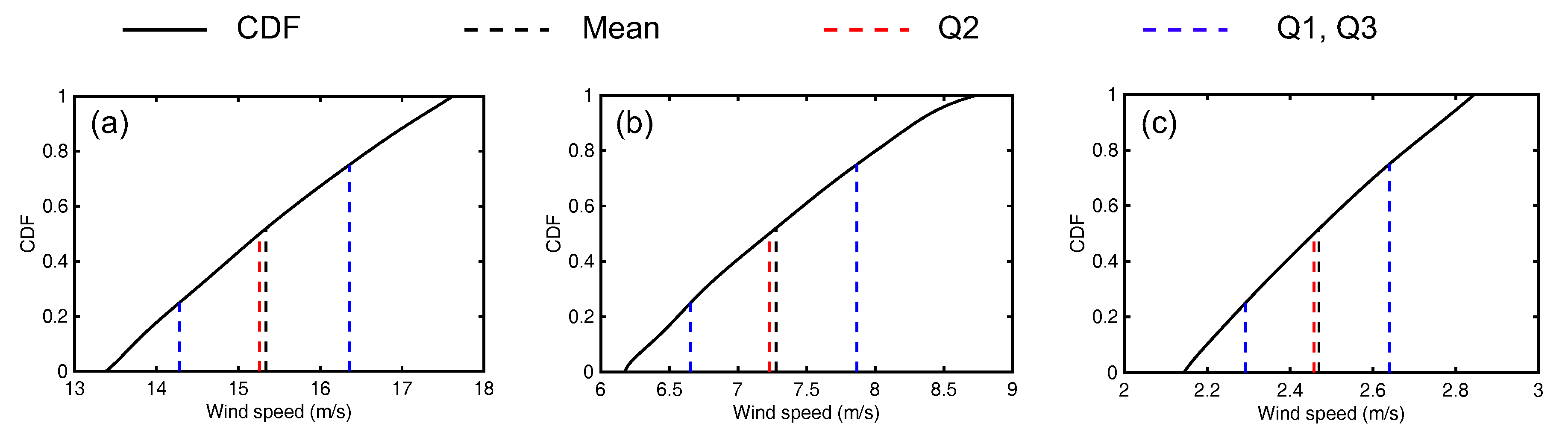
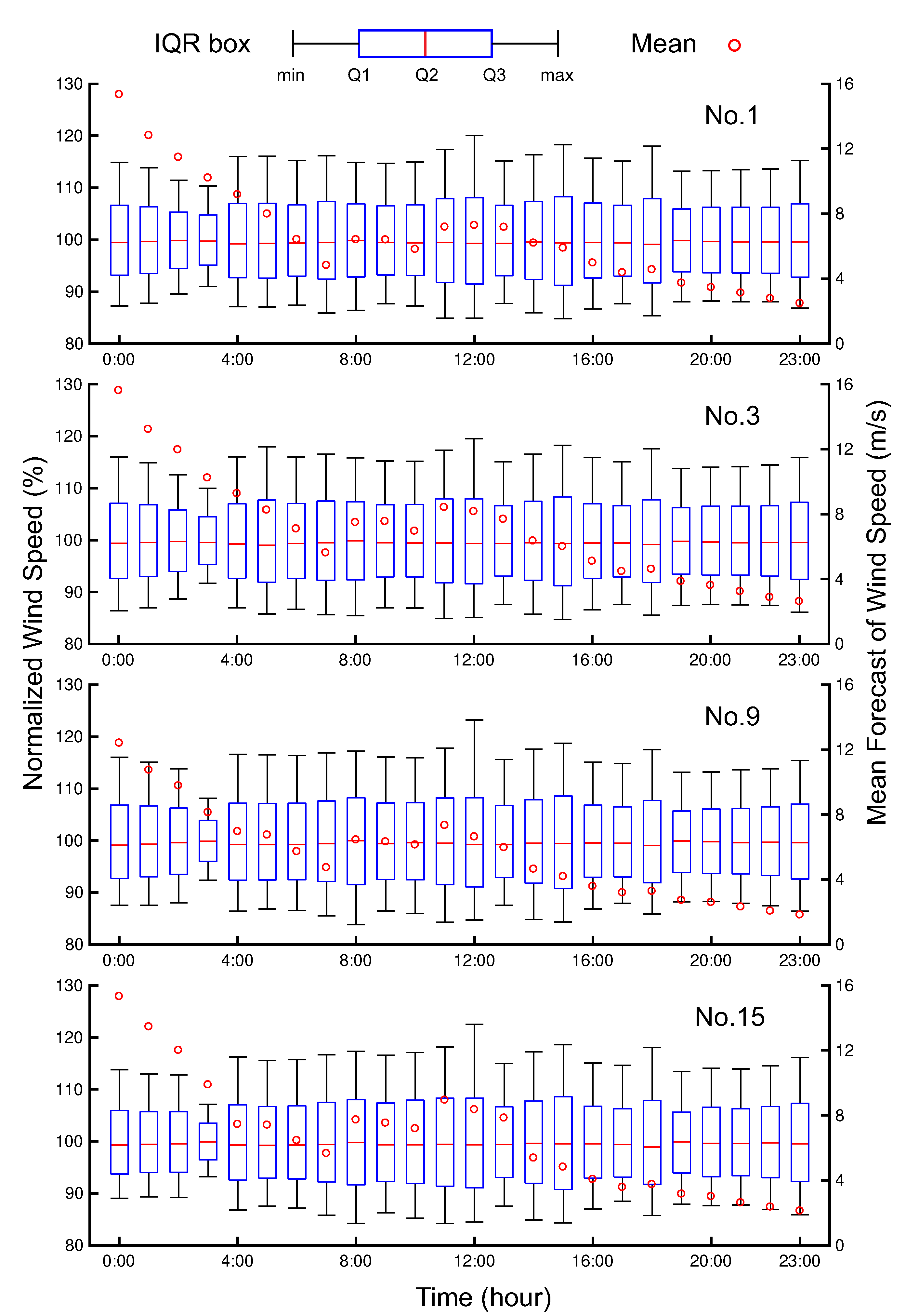
4.3.2. Statistic Characteristics of the Uncertainty in the Inflow Profile Parameter $\alpha$

As discussed above, the inlet wind profile plays a prominent role in predicting the wind field. We in this section discuss further the statistics of the wind speed prediction with the uncertainty in parameter $\alpha$. Figure 6 shows the wind speed change with the wind profile parameter $\alpha$ for three cases at the sites of turbine No.1, No.3, No.9, and No.15, respectively. The markers indicate the 17 quadrature points in the stochastic collocation method adopted in this study, and the black lines stand for the reconstructed profiles using the results of the stochastic collocation method. It is found that the reconstructed wind variation with respect to parameter $\alpha$ can be accurately fitted by the basis functions with the coefficients determined from the stochastic collocation method. From the reconstructed profiles, the relationship between $\alpha$ and the wind speed of each turbine can be obtained. Using this reconstructed profile and the predetermined probability function of the uncertainty element $p\left(\xi \right)$ (a uniform distribution within $[-1,1]$ in the present work), we can get the statistic properties of the predicted wind speed under the influence of uncertainty in $\alpha$.

The CDF functions of the corresponding wind speed of the three cases at turbine No.1 site are depicted in Figure 7 as an example, where we also indicate the mean value location and the points Q1, Q2, and Q3 standing for the locations where the CDF value equals to 25%, 50%, and 75%, respectively. It is observed that in all cases the CDF functions are slightly curved, and the mean value point locates close to but does not coincide exactly with the 50% CDF point, which indicates a weak nonlinearity in the CFD prediction results with respect to the uncertainty in $\alpha$.

The effects of the uncertain parameter $\alpha$ for four wind turbines at 24 instants, hourly from 00:00 UTC 9 October to 23:00 UTC 9 October 2013, are represented as the interquartile range IQR box and mean forecast of wind speed in Figure 8. The IQR values are based on the wind speed normalized with the mean values. It is notified that larger discrepancy between the wind forecasts of coupled model and observations is found during this period of time as shown in Figure 3.

Consistent with Figure 7, the difference between median and the mean wind speed is very small (≤1.13%). Although the IQR box varies among the turbines at different instants, the effect of the change of $\alpha$ is overall significant. For example, at instant 15:00, the significant variation in the normalized wind speed of turbine No.15 site for Q1 point reaches 9.26%, while that for Q3 point is 8.58%. Note that this kind of effect is prominent no matter how small or large the mean of wind speed forecast is. This significance of parameter $\alpha$ in affecting the wind speed forecast implies a potential to use it as the parameter for data assimilation to improve the numerical results of the coupled model.

5. Conclusions

In this study, a coupled model consisting of mesoscale WRF model and microscale OpenFOAM CFD model has been proposed to predict the hub-height wind at a wind farm in Japan, where the terrain condition is very complex and generates large fluctuations in surface wind field. The predicted hub-height wind of the coupled model has been compared with the raw prediction of WRF model as well as the observation, for a real-case test from 00:00 UTC 1 October to 23:00 UTC 9 October 2013. It is found that the coupled model is able to resolve more accurately the fine flow structures over the complex terrain. The numerical results show that the coupled model significantly ameliorates the hub-height wind forecasts in comparison with WRF-alone forecasts, with 26%, 22% and 4% improvements in the quantified metrics of ME, RMSE and CC, respectively.

In order to explore the possibility for further improvement, we have carried out the uncertainty quantification to analyze the sensitivity in the forecast wind speed to some important model parameters. A stochastic collocation method based on polynomial chaos expansion (PCE) has been used to obtain the statistics of the numerical results with uncertainties in constants of the turbulence model ($k-ϵ$ model) and the wind profile parameter $\alpha$ in the inflow conditions of the coupled model. It is found that the surface wind speed prediction from the coupled model is much more sensitive to parameter $\alpha$ than other parameters in the turbulence model. The uncertainties in the five parameters lead to weak impact on wind direction forecasts. The present work sheds a light on the importance of the inflow conditions for the CFD model, and suggests the next step to further improve the wind speed forecasting skill of the coupled model. A system to assimilate parameter $\alpha$ using the observation data of the target wind farm is under development.

References

1. Storm, B.; Basu, S. The WRF model forecast-derived low-level wind shear climatology over the United States Great Plains. Energies 2010, 3, 258–276. [Google Scholar] [CrossRef]
2. Chadee, X.T.; Seegobin, N.R.; Clarke, R.M. Optimizing the Weather Research and Forecasting (WRF) Model for Mapping the Near-Surface Wind Resources over the Southernmost Caribbean Islands of Trinidad and Tobago. Energies 2017, 10, 931. [Google Scholar] [CrossRef]
3. Zajaczkowski, F.J.; Haupt, S.E.; Schmehl, K.J. A preliminary study of assimilating numerical weather prediction data into computational fluid dynamics models for wind prediction. J. Wind Eng. Ind. Aerodyn. 2011, 99, 320–329. [Google Scholar] [CrossRef]
4. O’Sullivan, J. Modelling Wind Flow over Complex Terrain. Ph.D. Thesis, ResearchSpace@Auckland, Auckland, New Zealand, 2012. [Google Scholar]
5. Blocken, B.; van der Hout, A.; Dekker, J.; Weiler, O. CFD simulation of wind flow over natural complex terrain: Case study with validation by field measurements for Ria de Ferrol, Galicia, Spain. J. Wind Eng. Ind. Aerodyn. 2015, 147, 43–57. [Google Scholar] [CrossRef]
6. Moreno, P.; Gravdahl, A.R.; Romero, M. Wind flow over complex terrain: Application of linear and CFD models. In Proceedings of the European Wind Energy Conference and Exhibition, Madrid, Spain, 16–19 June 2003. [Google Scholar]
7. Wyszogrodzki, A.A.; Miao, S.; Chen, F. Evaluation of the coupling between mesoscale-WRF and LES-EULAG models for simulating fine-scale urban dispersion. Atmos. Res. 2012, 118, 324–345. [Google Scholar] [CrossRef]
8. Wang, Z.H.; Bou-Zeid, E.; Smith, J.A. A coupled energy transport and hydrological model for urban canopies evaluated using a wireless sensor network. Q. J. R. Meteorol. Soc. 2013, 139, 1643–1657. [Google Scholar] [CrossRef]
9. Miao, Y.; Liu, S.; Chen, B.; Zhang, B.; Wang, S.; Li, S. Simulating urban flow and dispersion in Beijing by coupling a CFD model with the WRF model. Adv. Atmos. Sci. 2013, 30, 1663. [Google Scholar] [CrossRef]
10. Miao, Y.; Liu, S.; Zheng, Y.; Wang, S.; Chen, B. Numerical study of the effects of topography and urbanization on the local atmospheric circulations over the Beijing-Tianjin-Hebei, China. Adv. Meteorol. 2015, 2015, 397070. [Google Scholar] [CrossRef]
11. Temel, O.; Bricteux, L.; van Beeck, J. Coupled WRF-OpenFOAM study of wind flow over complex terrain. J. Wind Eng. Ind. Aerodyn. 2018, 174, 152–169. [Google Scholar] [CrossRef]
12. García-Sánchez, C.; Philips, D.; Gorlé, C. Quantifying inflow uncertainties for CFD simulations of the flow in downtown Oklahoma City. Build. Environ. 2014, 78, 118–129. [Google Scholar] [CrossRef]
13. García-Sánchez, C.; Gorlé, C. Uncertainty quantification for microscale CFD simulations based on input from mesoscale codes. J. Wind Eng. Ind. Aerodyn. 2018, 176, 87–97. [Google Scholar] [CrossRef]
14. Che, Y.; Peng, X.; Delle Monache, L.; Kawaguchi, T.; Xiao, F. A wind power forecasting system based on the weather research and forecasting model and Kalman filtering over a wind-farm in Japan. J. Renew. Sustain. Energy 2016, 8, 013302. [Google Scholar] [CrossRef]
15. Launder, B.E.; Spalding, D.B. The numerical computation of turbulent flows. Comput. Methods Appl. Mech. Eng. 1974, 3, 269–289. [Google Scholar] [CrossRef]
16. Martinez, B. Wind Resource in Complex Terrain with OpenFOAM; Risø DTU, National Laboratory for Sustainable Energy: Roskilde, Denmark, 2011. [Google Scholar]
17. Stensrud, D.J.; Skindlov, J.A. Gridpoint predictions of high temperature from a mesoscale model. Weather Forecast. 1996, 11, 103–110. [Google Scholar] [CrossRef]
18. Hacker, J.P.; Rife, D.L. A practical approach to sequential estimation of systematic error on near-surface mesoscale grids. Weather Forecast. 2007, 22, 1257–1273. [Google Scholar] [CrossRef]
19. Xiu, D. Efficient collocational approach for parametric uncertainty analysis. Commun. Comput. Phys. 2007, 2, 293–309. [Google Scholar]
20. Xiu, D.; Karniadakis, G.E. The Wiener–Askey polynomial chaos for stochastic differential equations. SIAM J. Sci. Comput. 2002, 24, 619–644. [Google Scholar] [CrossRef]
21. Trefethen, L.N. Is Gauss quadrature better than Clenshaw–Curtis? SIAM Rev. 2008, 50, 67–87. [Google Scholar] [CrossRef]
22. Richards, P.; Hoxey, R. Appropriate boundary conditions for computational wind engineering models using the k-ε turbulence model. In Computational Wind Engineering 1; Elsevier: Amsterdam, The Netherlands, 1993; pp. 145–153. [Google Scholar]
23. Rehman, S.; Al-Hadhrami, L.M.; Alam, M.M.; Meyer, J. Empirical correlation between hub height and local wind shear exponent for different sizes of wind turbines. Sustain. Energy Technol. Assess. 2013, 4, 45–51. [Google Scholar] [CrossRef]
24. Edeling, W.; Cinnella, P.; Dwight, R.P.; Bijl, H. Bayesian estimates of parameter variability in the k–ε turbulence model. J. Comput. Phys. 2014, 258, 73–94. [Google Scholar] [CrossRef]
Figure 1. The configuration of inner most Weather Research and Forecasting (WRF) domain (a) and the OpenFOAM domain (b). The gray shaded indicates the terrain height. An enlarged part of the mesh structure of OpenFOAM domain is displayed in (c), where the wind farm of interest is included. The red triangles stand for the specific position of 15 turbine sites.
Energies 12 01505 g001
Figure 2. The distributions of the pressure (a) and the wind velocity (b) at 12:00 a.m. UTC, 1 October 2013, over the target area where the x and y represent the east and north directions, respectively. Two vertical cross sections are also included to provide 3D images. The dominant wind direction is northwestern.
Energies 12 01505 g002
Figure 3. The WRF forecasts (“WRF_fore”), the predictions of the coupled system (“WRF+OpenFOAM”) and the corresponding observations (“OBS”) of seven turbines for 192 cases, from 00:00 UTC 2 October to 23:00 UTC 9 October 2013.
Energies 12 01505 g003
Figure 4. Same as the Figure 3, but for the turbines from No. 8 to No. 15.
Energies 12 01505 g004
Figure 5. A comparison of mean error (ME) (a), root mean square error (RMSE) (b) and correlation coefficient (CC) (c) of the WRF model (solid black bar), the running mean method (solid white bar) and the coupled model (solid gray bar) forecasts of wind speed for the 15 turbines of the Awaji-island wind farm in Japan. The red line stands for the relative improvement by WRF/OpenFOAM coupled model in comparison with the WRF-alone forecasts and the forecasts using running mean approach.
Energies 12 01505 g005
Figure 6. The quadrature points and reconstructed profiles on the stochastic domain for turbine No.1 (a), No.3 (b), No.9 (c), and No.15 (d). The black lines are the reconstructed profiles via the stochastic collocation method using the values at the quadrature points.
Energies 12 01505 g006
Figure 7. The cumulative distribution functions (CDFs) of the wind speed at turbine No.1 site for case1 (a), case2 (b) and case3 (c). Mean value location is indicated by the black dotted line, and Q2 location (CDF value equals to 50%) by red dotted line. The left-most dotted blue line indicates the Q1 location (CDF value equals to 25%), while the right-most dotted blue line indicates the Q3 location (CDF value equals to 75%), respectively.
Energies 12 01505 g007
Figure 8. The interquartile range (IQR) boxes of the wind speed normalized by the mean values (left axis) in regard to the uncertainty in α for four turbines at 24 instants from 00:00 UTC 9 October to 23:00 UTC 9 October 2013. In each box, minimum, Q1, Q2, Q3, and maximum value stand for the CDF 0%, 25%, 50%, 75%, and 100%, respectively. The red circles indicate mean values of the wind speed forecasts (right axis) for each time instant.
Energies 12 01505 g008