1. Introduction
According to a Global Status Report 2017 [
1], buildings account for 28% of global carbon dioxide emissions, and are a significant contributor to climate change. A recently published report by the Intergovernmental Panel on Climate Change [
2] stresses the need for urgent action to reduce global carbon emissions, and intervention on buildings therefore needs to form a significant part of this effort. With only 1% of new buildings in the UK building stock, it is clear that existing buildings have the greatest impact on climate change and need to become the focus of structured improvement programs.
But how do we know the extent to which to improve an existing building? It is critical to establish thermal properties of an existing building accurately in order to be able to design performance improvements with confidence. There are two types of physical tests that can be carried out on a building that enable thermal properties to be determined: a co-heating test [
3], p. 251, and a dynamic heating test [
3], p. 259. The former involves heating a building with supplementary electric heaters over a period of several days, as well as monitoring internal and external air temperatures and the consumed electricity energy, resulting in the calculation of the overall heat loss coefficient. However, during the heating-up part of the co-heating test, the building goes through a dynamic change of internal temperature, and this can enable the calculation of two more properties: the time constant, and the effective thermal capacitance of the building [
4], thus going beyond steady-state thermal properties into dynamic physics properties.
Whilst there is a body of published work on co-heating tests, the focus of much of the work is on the procedures [
5] and repeatability of results [
6]. Thus, Jack et al. [
6] reported on co-heating tests conducted by seven different teams on the same building, achieving the measurement of heat loss coefficient within ±10% of the mean. Staford et al. [
7] conducted 34 co-heating tests on 21 dwellings and found discrepancies of up to 120% between predicted and measured heat losses. Farmer and co-workers used a fully instrumented house located within a test laboratory to measure thermal performance in steady-state conditions at each stage of a full-fabric retrofit of a solid wall dwelling [
8]. They found an increased accuracy of their measurements in comparison with the measurements in the field, although the absence of wind in the test facility and the incomplete thermal bridging calculations made it difficult to compare the measurements with heat loss coefficient predictions.
A dynamic method for measurement of the whole building heat loss was reported by Alzetto and co-workers [
9]. They claim “reasonable accuracy” of the estimated heat loss coefficient, obtained on the basis of a dynamic experiment of less than one-night duration. However, these results are questionable, as building time constant is generally a lot longer than the length of one night (explained in
Section 3 and
Section 4 of this article). Mangematin et al. [
10] developed a dynamic method for a quick measurement of the energy efficiency of buildings. In four experiments that lasted one or two days, they obtained high consistency of the heat loss coefficient and effective thermal capacitance values between all experiments. They found their experimental measurement of the heat loss coefficient, conducted in a new house, was almost identical to the calculated value, as result of the newbuild homogeneous envelope and uniform heat input covering the entire floor. Roels at al. [
11] worked on a method for characterizing the actual thermal performance of buildings as part of an IEA EBC Annex 58 project on “Reliable Building Energy Performance Characterisation Based on Full Scale Dynamic Measurements” [
12]. Whilst most of this work was based on test facilities, discrepancies of up to 360% were found between measured and theoretical values, mainly as result of poor workmanship.
Both co-heating and dynamic heating tests are considered to be disruptive—the building needs to be unoccupied for at least a week, internal gains need to be set to zero, and the external weather conditions need to be cold and reasonably stable over the period of the test. Considering that weather conditions may change significantly during the test and could make the results inconclusive, the repetition of the tests would require the building to be unoccupied over a longer period of time. These tests are restricted to winter time and any repetition of the tests may overrun into a warmer period when the tests will not be possible to do.
This disadvantage of actual physical testing can be overcome by having an accurate simulation model of the building and carrying out a simulation of the dynamic heating test during the winter period of the simulation weather file. Simulation models can be considerably inaccurate, resulting in a performance gap between simulated and actual behavior; however, they can also be calibrated to almost completely eliminate the performance gap. In order to obtain the data for the calibration of a simulation model, instrumental monitoring of the building energy performance is required. A simulation weather file will need to be amended with actual measured data to facilitate the calibration process. Alternatively, good annual records of energy bills would be required.
This article introduces physical dynamic heating tests in an unoccupied building, and simulated dynamic heating tests in an occupied building, and documents and discusses the results. In the case of the occupied building, the simulated dynamic heating tests were carried out before and after deep energy retrofitting, and the change of building physics properties through the retrofit is documented.
This research gives new insights into the properties of building materials in use, in contrast with their published values determined through laboratory testing under controlled conditions. It enables more realistic design improvements to be made through deep energy retrofitting. Accurate information on the building physics properties enables the development of simplified but accurate dynamic models of buildings, which can run in a microprocessor, determine the physics parameters through machine learning, and carry out energy-saving predictive control [
13].
The methods introduced in this article can also be used for quality assurance of deep energy retrofit projects, on the basis of measurement of building physics properties before and after the retrofit, and establishing whether the risk of higher U-values than in the manufacturers’ specifications is properly dealt with.
2. Method
The method in this research consists of two parts: physical dynamic heating tests in a building, and the calibration of a dynamic simulation model of the building before and after the retrofit and carrying out dynamic heating test simulations with the calibrated models.
In both parts, internal air temperature is obtained starting from a simplified heat balance equation, adapted from Jankovic [
3], p. 261:
The solution of Equation (1) can be expressed as:
Equation (2) can be expressed as follows:
The time constant is subsequently determined from curve fitting Equation (3) by minimizing the root-mean-squared error defined as
The overall heat loss coefficient is then calculated as
from the steady-state part of the dynamic heating test (
Figure 1).
As
tc becomes known from the curve-fitting procedure, and as the overall heat loss coefficient
HLC becomes known from Equation (5), effective thermal capacitance is calculated as
Therefore, the results of the dynamic heating test consist of the building time constant tc, effective thermal capacitance C, and the overall heat loss coefficient HLC.
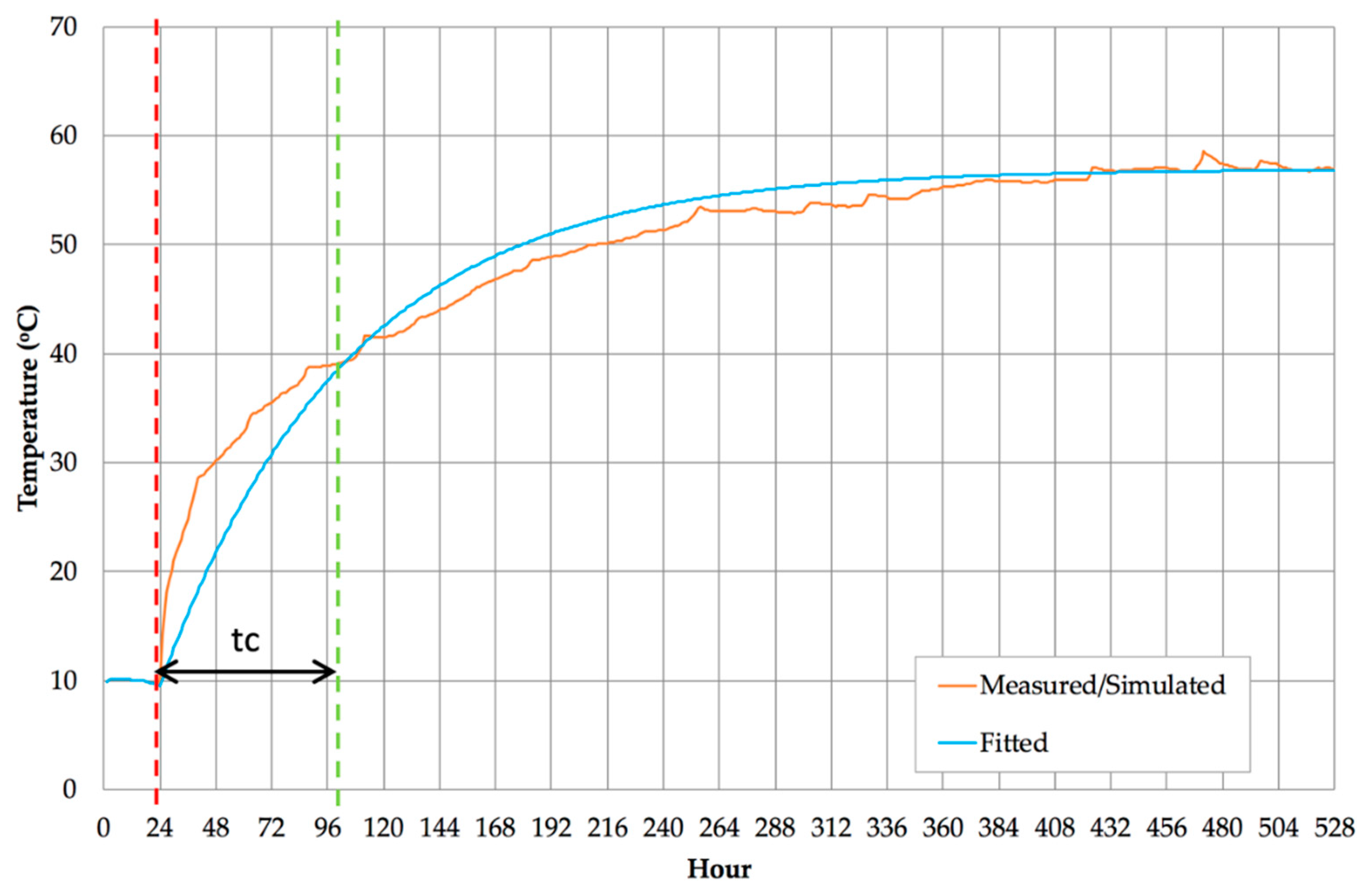
This method is illustrated in
Figure 1, where a curve is fitted to the result of the test, and where the time constant, which represents the time needed to go through 63% of the total change of temperature, is denoted as the time between the vertical red and green lines. The
HLC value is obtained from the asymptotic part of the fitted curve as a ratio between the heat input and the temperature difference between the inside and outside.
In the case of the physical test, the curve fitting is carried out with reference to measured internal temperatures as per Equations (3) and (4), and in the case of the simulated test, the curve fitting is carried out with reference to simulated internal temperatures using the same equations.
The simulated dynamic heating test needs to be carried out with a calibrated simulation model. The calibration is carried by minimizing relative errors between measured and simulated energy consumption, where objective functions are as follows:
The minimization is carried out using parametric simulation and multi-objective optimization, with two separate objective functions corresponding to thermal and electrical energy consumption based on Equation (7). The parameters for parametric simulations are: several variations of external wall and roof construction types, so that the thickness of thermal insulation is varied in each construction below and above the actual insulation thickness in order to determine the effective value of thermal insulation; a range of values of air tightness; a range of values for internal set temperature; a range of values of electrical lighting power density; and a range of values of miscellaneous gains power density. The parametric simulations and multi-objective optimization create a scatter plot of simulation model results (
Figure 2), and the point that is the closest to the origin of the coordinate system corresponds to a model with minimum errors—the calibrated model.
The calibrated model is subsequently used for conducting simulated dynamic heating tests. Details of the results of calibration of a specific building before and after the retrofit are provided in
Section 4.
A point worth noting is that multi-objective optimization reduces the number of simulation runs in comparison with parametric simulation runs. Instead of running the parametric simulations exhaustively for every combination of different parameters, such as construction types, air tightness, heating set temperatures, and so on, multi-objective optimization uses a genetic algorithm NSGA-II [
14] to search only the most viable parts of the solution space. Thus, the total search space for parametric simulations was just over 920,000 simulation cases, and only 737 cases were selected by the genetic algorithm as the most viable.
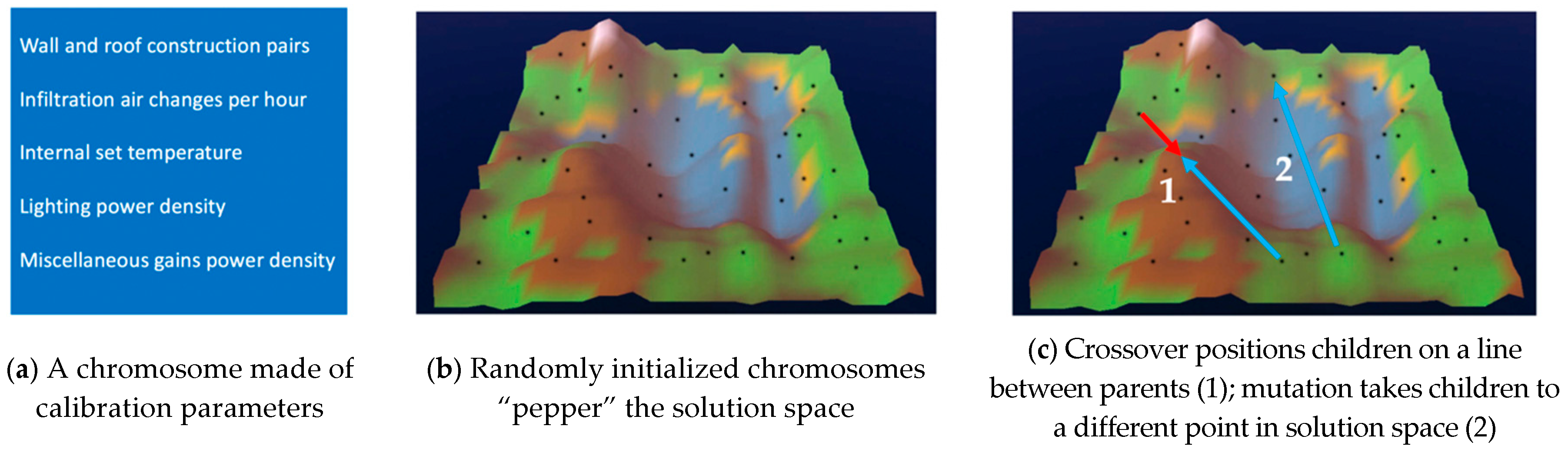
The reduction from 920,000 cases to 737 cases is now explained in more detail. The genetic algorithm used in the background of the parametric simulations treats each calibration parameter as a gene, and the combination of all parameters as a chromosome (
Figure 3a). The first generation of chromosomes is created by assigning random values of each calibration parameter within the range specified in
Section 4. The result is that the entire multidimensional solution space, conceptually represented in
Figure 3b as three-dimensional, is “peppered” with random chromosomes, where each chromosome represents an annual performance simulation using EnergyPlus [
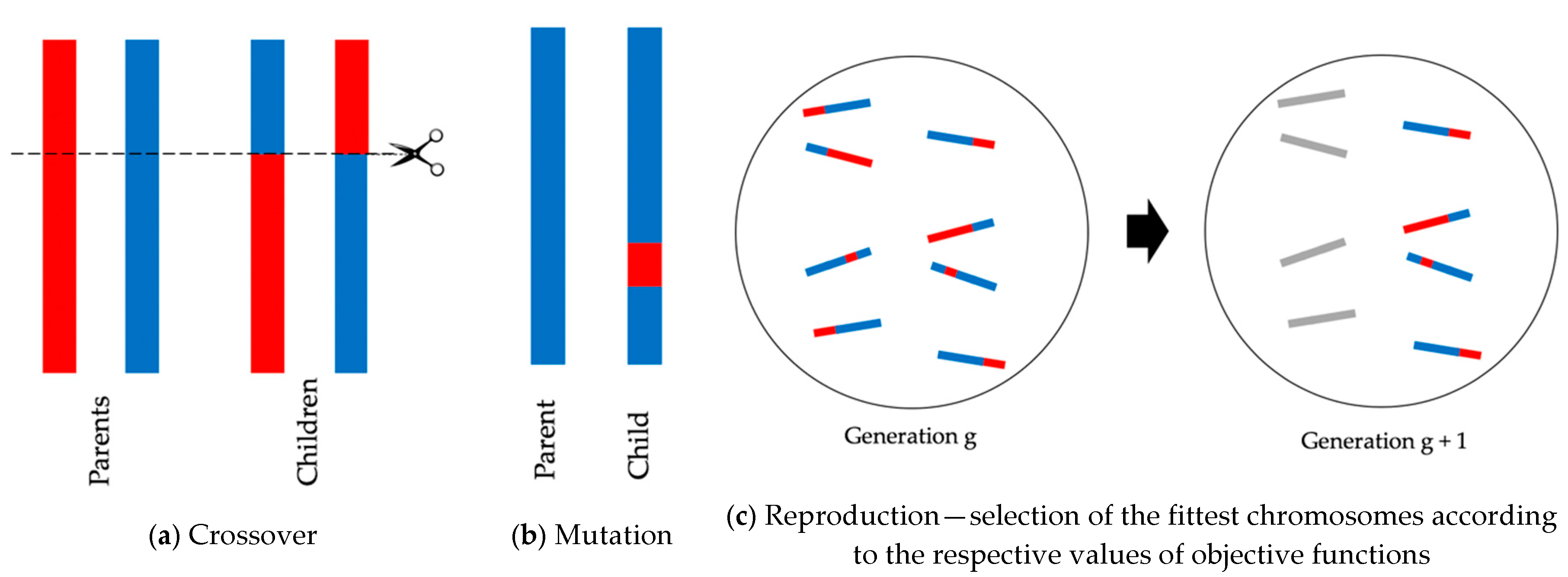
15]. This is where genetic operations of crossover, mutation, and reproduction start, as illustrated in
Figure 4. Two randomly selected chromosomes are paired, and split at a random position and crossed over to create a new child (
Figure 4a). That new child is on a straight line between the parents in the solution space (
Figure 3c(1)). Occasionally, a new child is created by mutation (
Figure 4b), which takes it to a different part of the solution space (
Figure 3c(2)). As EnergyPlus simulations proceed, the fitness of each chromosome is evaluated using Equation (7), and the fittest chromosomes are transferred into the next generation, while the unfit chromosomes, shown in grey in
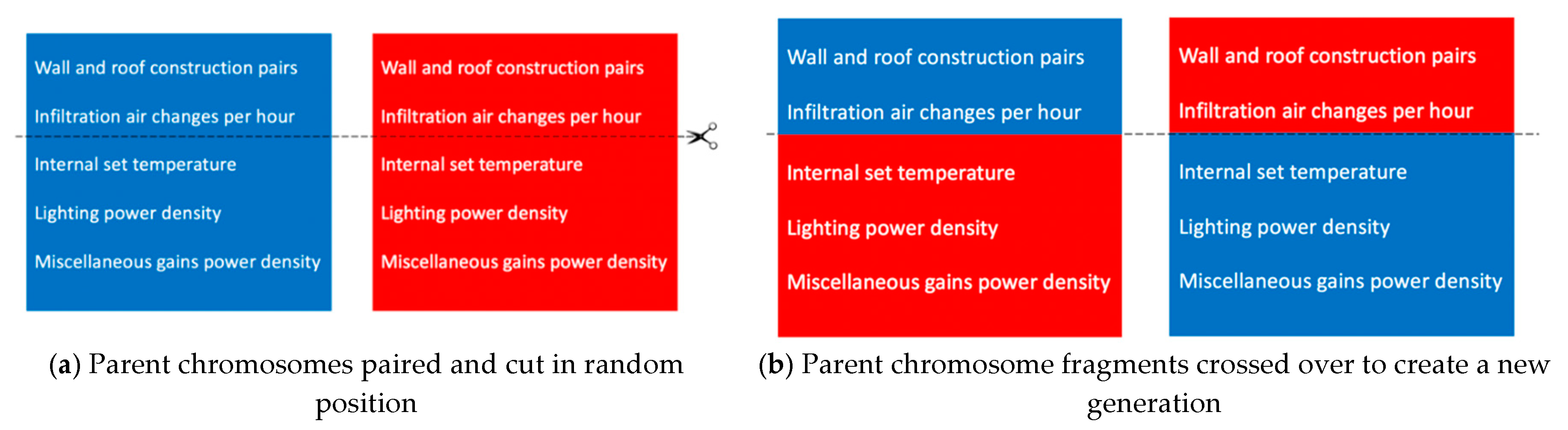
Figure 4c, are discarded according to the values of objective functions in Equation (7). This represents the operation of reproduction. As the process repeats a generation after a generation, the discarding of unfit chromosomes results in the reduction of simulation cases to be run, thus explaining the reduction from 920,000 to 737 cases in the particular example.
Calibration parameters in chromosome crossover are illustrated in
Figure 5.
The results of this process are shown on a scatter plot, and the model with the lowest relative error is subsequently selected from the scatter plot in
Figure 2.
3. Physical Dynamic Heating Test Experiments and Results
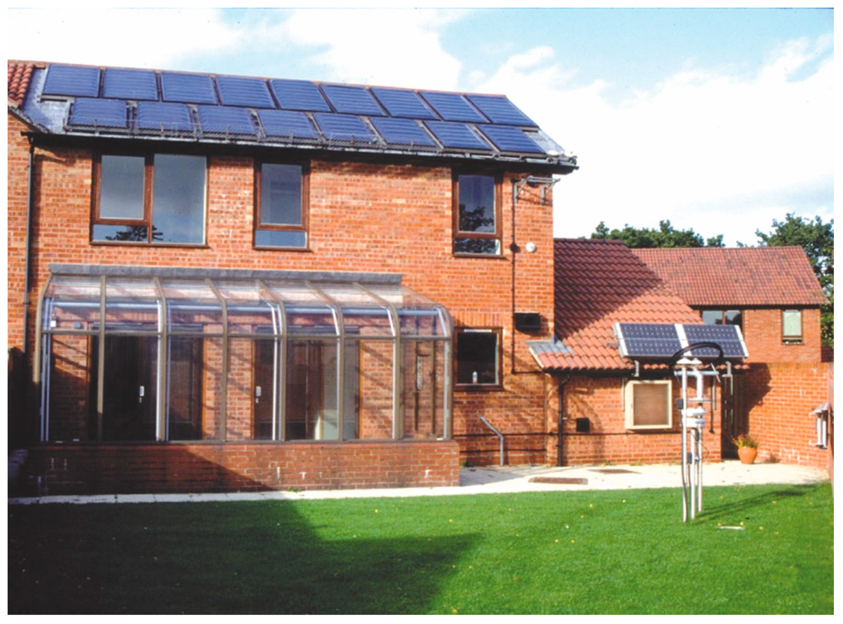
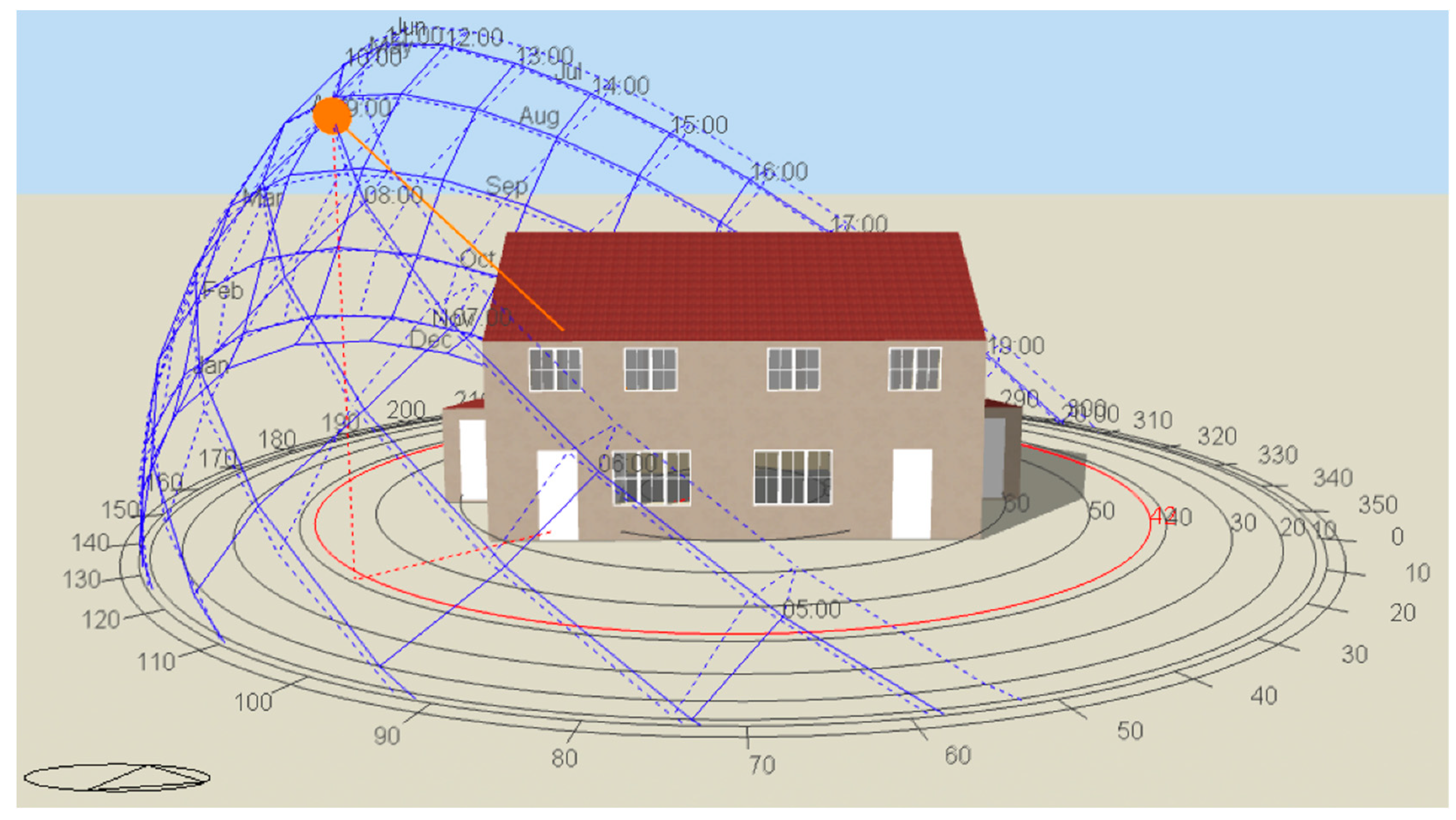
Physical dynamic heating tests were conducted on a Solar Demonstration House in Bournville, Birmingham (
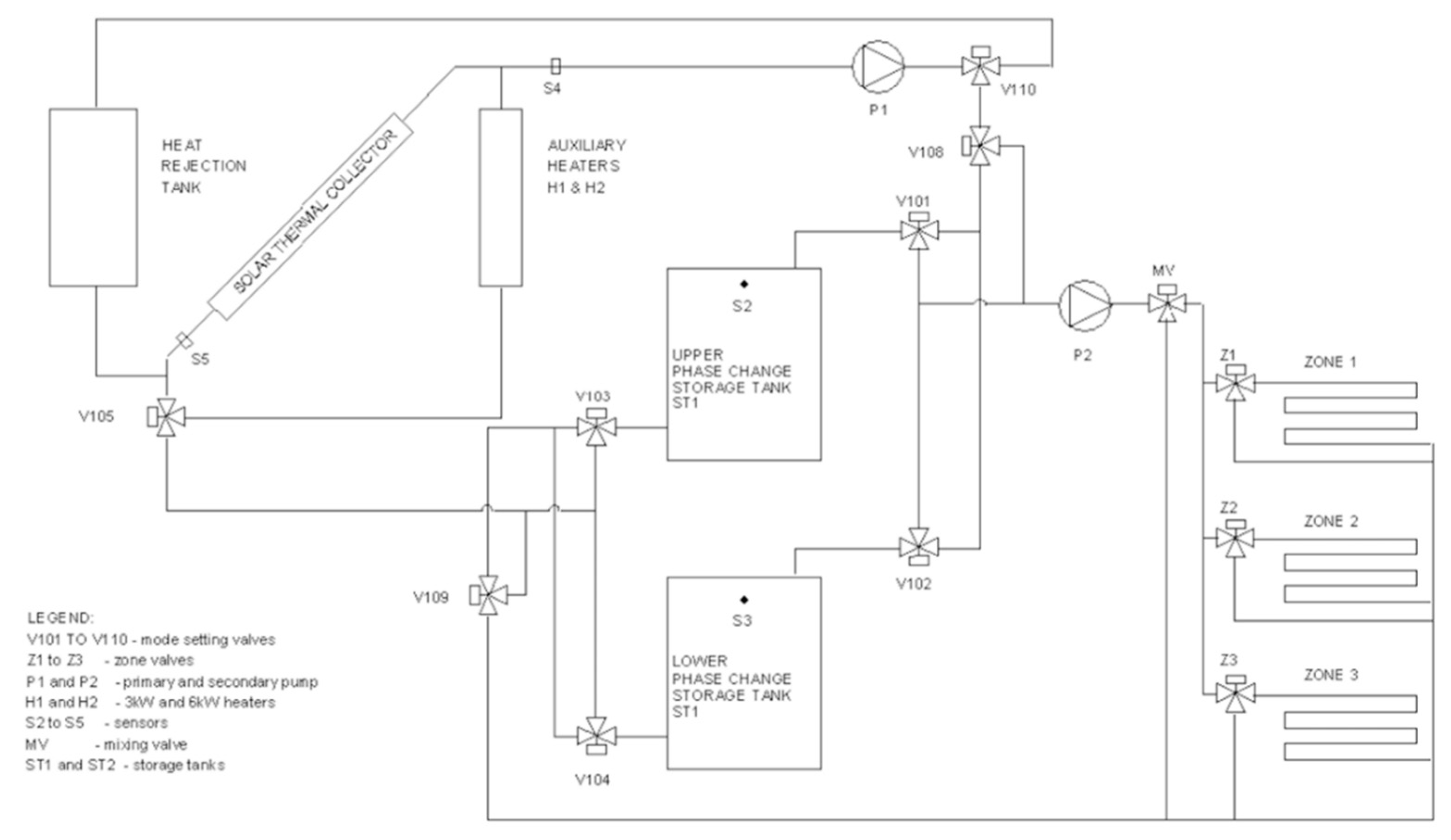
Figure 6). The house was based on a brick and block construction with a 100-mm cavity filled with polystyrene beads. The building was designed to absorb passive solar gain in the internal layer of external walls (consisting of high-density concrete blocks), and in the ground and first floor concrete slabs. Gas heating combined with an active solar thermal system supplied heat to two large storage tanks fitted with phase-change material, and heat was then distributed to the internal space via underfloor heating (
Figure 7). The heat indirectly absorbed in the storage tanks had to be taken into account in the analysis of results of dynamic heating tests.
The house was heavily instrumented for research purposes, in order to monitor various aspects of building performance. This included a weather station with two pyranometers measuring horizontal total and diffuse solar radiation, external air temperature and relative humidity (
Figure 6), plus over 200 internal sensors measuring various temperatures and other parameters in the building fabric and in the solar thermal system.
The building was subjected to a series of dynamic tests according to the schedule given in
Table 1. Each test consisted of a heating and cooling part. The time of the beginning of the heating part of each test was the time when heating was switched on, introducing a step change to the heat input. Additional electric heaters were used in combination with the house underfloor heating system for the dynamic heating tests.
The indoor air temperatures recorded during the heating part of the tests are shown in
Figure 8. The starting temperature
Tstart has been normalized to the same value of 10 °C for all six tests, with a corresponding adjustment for the outside temperature so that the temperature difference between inside and outside remained the same as measured. The cooling part of the tests started at the time the heaters were switched off. The building had been allowed to cool down to a free floating indoor temperature before the heating part of each test. The indoor air temperature was calculated as a volume-weighted average of all measured room temperatures. An occurrence of steady room temperature was used as a criterion for the end of the heating part of each test. The influence of solar radiation on the building response was reduced by means of thermal blinds. These were specially designed for this purpose, with a reflective outside surface and a thermally insulating fabric with edge seals.
Curves fitted to the indoor air temperatures data of the heating part of each test are shown in
Figure 9.
The reason for the choice of both underfloor heating and electric heating (
Table 1) was to expose the building to a wider range of heat inputs. As the tests with electric heating only (Tests 2 and 6,
Table 1) show similar time lags to the tests with underfloor heating switched on, there does not seem to be any significant difference between the two types of heat inputs. As the building was heavily instrumented, underfloor heating contribution was easy to measure. Any input that did not directly contribute to the internal temperature change is accounted for in
Table 2 under “Power Absorbed by Storage Tanks”. Related work shows good agreement between heat loss coefficients obtained from co-heating tests conducted with electric heaters and with a building’s own heating system [
17], thus justifying the approach in this article.
There were several difficulties encountered during the tests. During Test 1, the electricity meters were not available, and the nominal power of the electric heaters was used in the calculations. The air tightness was not known during Tests 1–4. This was calculated as the air tightness corresponding to the minimum relative error of the calculations. The air tightness was subsequently measured between Tests 4 and 5 after the air-tightening of the building had been carried out. The air tightness during Tests 5 and 6 was therefore known, and it was n = 0.68 1/h. Test 4 could not be conducted properly, as the high-limit thermostat in the heating system cut the power off long before the occurrence of the asymptotic room temperature. The data from this test have not been used for the calculation of the final results of the series of tests as the test result was based on extrapolated calculations and insufficient information on heat losses.
A further complication was that the measured heater power was different from the nominal in Test 3 (3.53 kW instead of 3 kW). The average total and auxiliary power were measured as different, although there was no any obvious reason for such difference. For this reason, two sets of calculations of the test results were carried out, one with the measured heater power in Test 3, and the other with the nominal heater power in the same test. In all other tests the measured power data were used, except in Test 1 where the electricity meters were not installed at the time of the test. A summary of heat input during the heating tests is shown in
Table 2.
In the following text, Case 1 refers to the analysis where the measured heater power in Test 3 (3.53 kW) was used, and Case 2 refers to the analysis where the nominal power in Test 3 was used (3 kW). The air tightness during Tests 1–4 had to be first assumed and determined from iterative calculations. Standard relative errors of the calculations of the heat loss coefficient HLC and the effective capacitance C are functions of the air tightness. These errors reached the minimum for the air tightness of n = 1.8 1/h in Tests 1–4 of Case 1. The minimum errors for Case 2 were reached for the air tightness of n = 1.2 1/h in Tests 1–4.
Results of dynamic heating tests are shown in
Table 3. As it can be seen from this table, multiple values have been obtained for each physics property.
The precision of the measurement of building physics properties would have been higher if additional weather data had been available, including wind speed at the building location, rain-caused evaporation effects on the building surface, measured air tightness for all experiments, and whether or not the ambient air temperature was truly constant. Under the circumstances the dynamic heating tests were conducted, and under the assumptions made during the analysis, it is possible to conclude that the building physics properties have the following values:
| Case 1: | tc = 44.4 ± 2.7 h
HLC = 256.2 ± 24.6 W/K
C = 41.1 ± 6.0 MJ/K | | Case 2: | tc = 46.4 ± 0.4 h
HLC = 268.5 ± 1.8 W/K
C = 44.8 ± 0.4 MJ/K |
As the assumptions for Case 1 appear to be more realistic, and as the range of associated results with their standard errors include the Case 2 results, the Case 1 results are considered to be the final results of the physical dynamic heating tests.
The ASHRAE Handbook of Fundamentals [
18] divides buildings into three categories: light, medium and heavy construction types, with respective capacitance of 112, 261 and 485 kJ/(K·m
2 of floor area). If we assume that the Demonstration House is in the heavy category due to high density concrete blockwork in the internal layer of the external walls, and due to concrete slabs, then the calculated capacitance for 83.7 m
2 of floor area is 40.6 MJ/K. The effective capacitance obtained from the experimental data is between 41.1 ± 6.0 MJ/K (
Table 4), and therefore within 1.3% relative error with reference to the theoretical value from the ASHRAE Handbook of Fundamentals [
18].
This, however, cannot be said for the overall heat loss coefficient. When its value is calculated on the basis of the published properties of building materials, the result comes to 172.9 W/K. This is an alarming fact for designers who rely only on building material properties published in manufacturers’ specifications and in engineering tables. The differences between theoretical end experimental values are shown in
Table 5, and are on average 48%, potentially reaching over 60%.
4. Simulated Dynamic Heating Test Experiments and Results
Conducting physical dynamic heating tests in a building is impractical and disruptive. The building needs to be unoccupied for the duration of the test so that no heat gains or heat losses occur as result of occupancy; furthermore, if the external weather conditions become unstable, the tests need to be repeated, leading to a prolonged time in which the building needs to be unoccupied. Recent developments have enabled occupants to live in the building during retrofit construction, whilst the quality control method does not quantify the improvements in the building envelope.
In this context, a method of simulated dynamic heating tests was developed, using the standard simulation tool EnergyPlus [
15] as a quality assurance procedure for a retrofit project carried out on two semi-detached houses owned by Birmingham City Council and based on “Wimpey No-fines” construction (
Figure 10).
That construction type was predominant in the UK in the late 1940s and early 1950s due to increased housing demand and a lack of skilled labor. The concrete was cast in situ so that the houses were quicker to build without requiring the skills of traditional building trades. As building regulations at that time did not require an energy-efficient design, this left a legacy of some 300,000 houses that now require deep energy retrofitting.
The method developed here was to provide an answer to a practical question of how to address the risk of higher U-values in the completed retrofit than those in the manufacturers’ specifications. The envelope characteristics before and after the retrofit, as reported by Jankovic [
19], are shown in
Table 6.
In the first step, a calibration of the simulation model before and after the retrofit was carried out using JEA [
20] running EnergyPlus as a simulation engine [
15], as illustrated in
Figure 2. Details of calibration parameters are in
Table 7. The choice of JEA was dictated by its capability for user-defined objective functions, which were in this case based on Equation (7a–d) for gas and electricity consumption.
Thus, specific objective functions in respect to gas and electricity consumption in the pre-retrofit case were obtained by substituting numerical values of measured annual energy consumption in Equation (7) as follows:
Similar substitution of monitored annual energy consumption in Equation (7) provided objective functions in the post-retrofit case as follows:
In both pre-retrofit and post-retrofit cases, numerical values in Equation (7a–d) are in Joules, in order to make the measured values units-compatible with EnergyPlus results. The simulated values in these equations were obtained by varying parameters in the EnergyPlus model, as per
Table 7, and the genetic algorithm controlled which EnergyPlus simulations were actually going to be run, with reference to the explanations of
Figure 3,
Figure 4 and
Figure 5.
The EnergyPlus model, required for running JEA, was developed using DesignBuilder [
21] (
Figure 11), and by exporting from it a text file called EnergyPlus Input Definition File (IDF), thus obtaining the EnergyPlus model.
The results of calibration are shown in
Table 8. In addition to the high accuracy of the calibrated model before and after the retrofit, two additional matters become apparent as a result of calibration after the retrofit: (1) the external wall thickness in the calibrated model of 256 mm (
Figure 2) differed from the actual thickness of 270 mm, indicating that the actual U-value would be higher than the theoretical (
Table 6); and (2) the calibration could not be completed with the measured air-tightness value of 1.78 1/h at 50 Pascal, as the calibration errors in respect to gas consumption were in excess of 5%. When air tightness was changed from the fixed value corresponding to the air tightness test result to a varying range of parametric values, the calibration errors were reduced to those reported in
Table 8, and the corresponding air tightness value obtained from the scatter plot in
Figure 2 was 0.8 1/h.
As gas energy was used for heating and electricity for lighting and plug loads, a minimization of errors in respect to these two sources of energy was carried out. The high accuracy of the calibrated models (
Table 8) confirmed their accurate representation of the building behavior and justified their use for dynamic heating tests. As the simulation models were calibrated using measured data, the dynamic heating tests with these models were considered to be a form of measurement. This was the basis for deciding that more than one dynamic test simulation would be required for the case before the retrofit and after the retrofit.
The initial choice of heat input in dynamic test simulations was consistent with the heat input in physical tests reported in
Section 3, namely 3, 6, 9, 12, and 15 kW. However, in the post-retrofit case, the heat input was overridden by the simulation tool without explicit instruction when internal temperatures of over 70 °C were reached, so that the corresponding results could not be considered to represent unconstrained building behavior. This behavior was attributed to internal limits of the simulation tool, occurring for heat input rates of 12 kW and above in the post-retrofit case. Therefore, the maximum heat input rate that resulted in the behavior driven by the building physics parameters alone was considered to be 9 kW in the post-retrofit case. Whilst there was no similar limitation to the pre-retrofit case (i.e., the test with 12 and 15 kW did not result in exceeding internal temperature limits), only the results of tests with 3, 6, and 9 kW have been analyzed for the cases before and after the retrofit for consistency reasons.
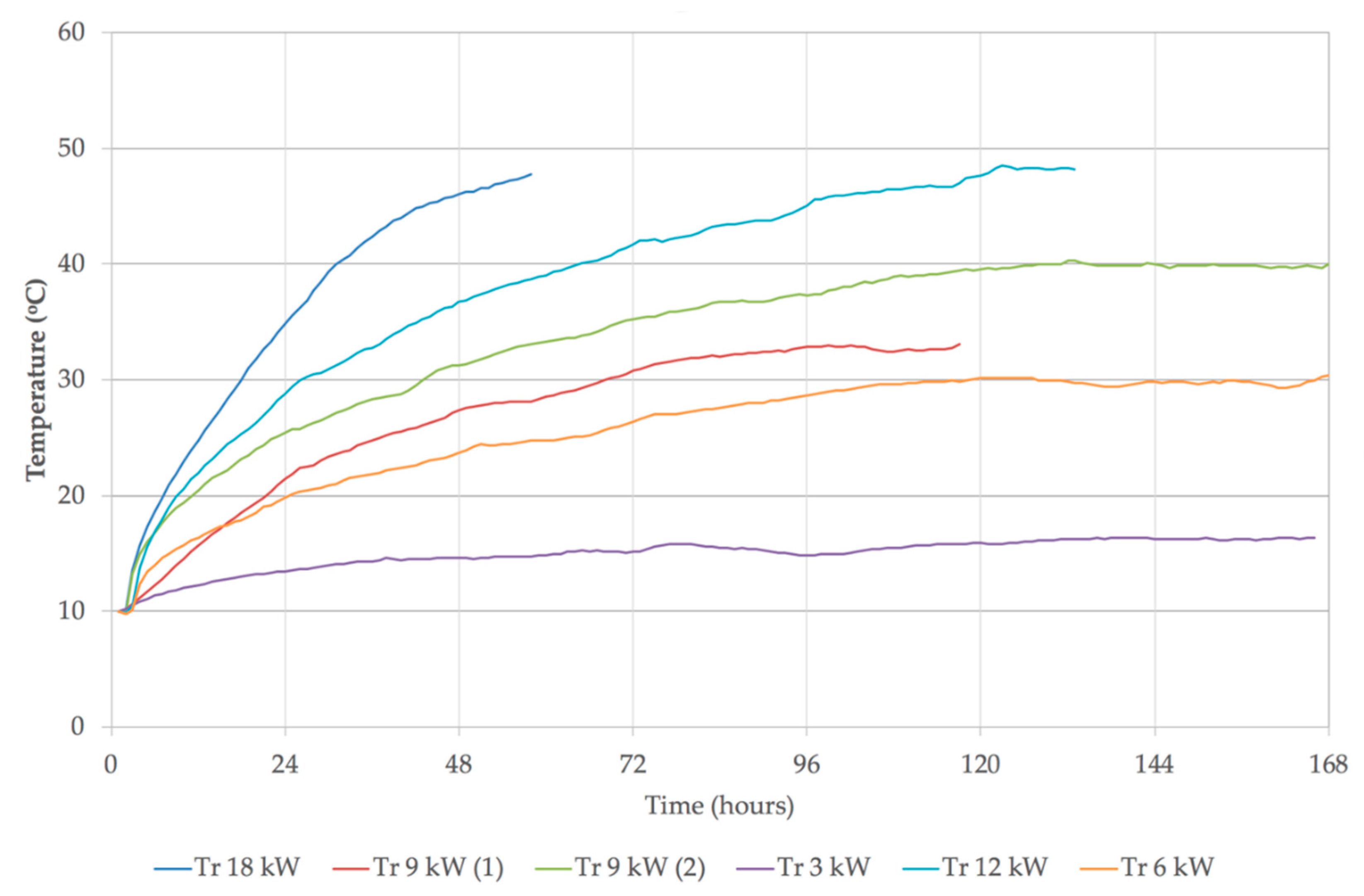
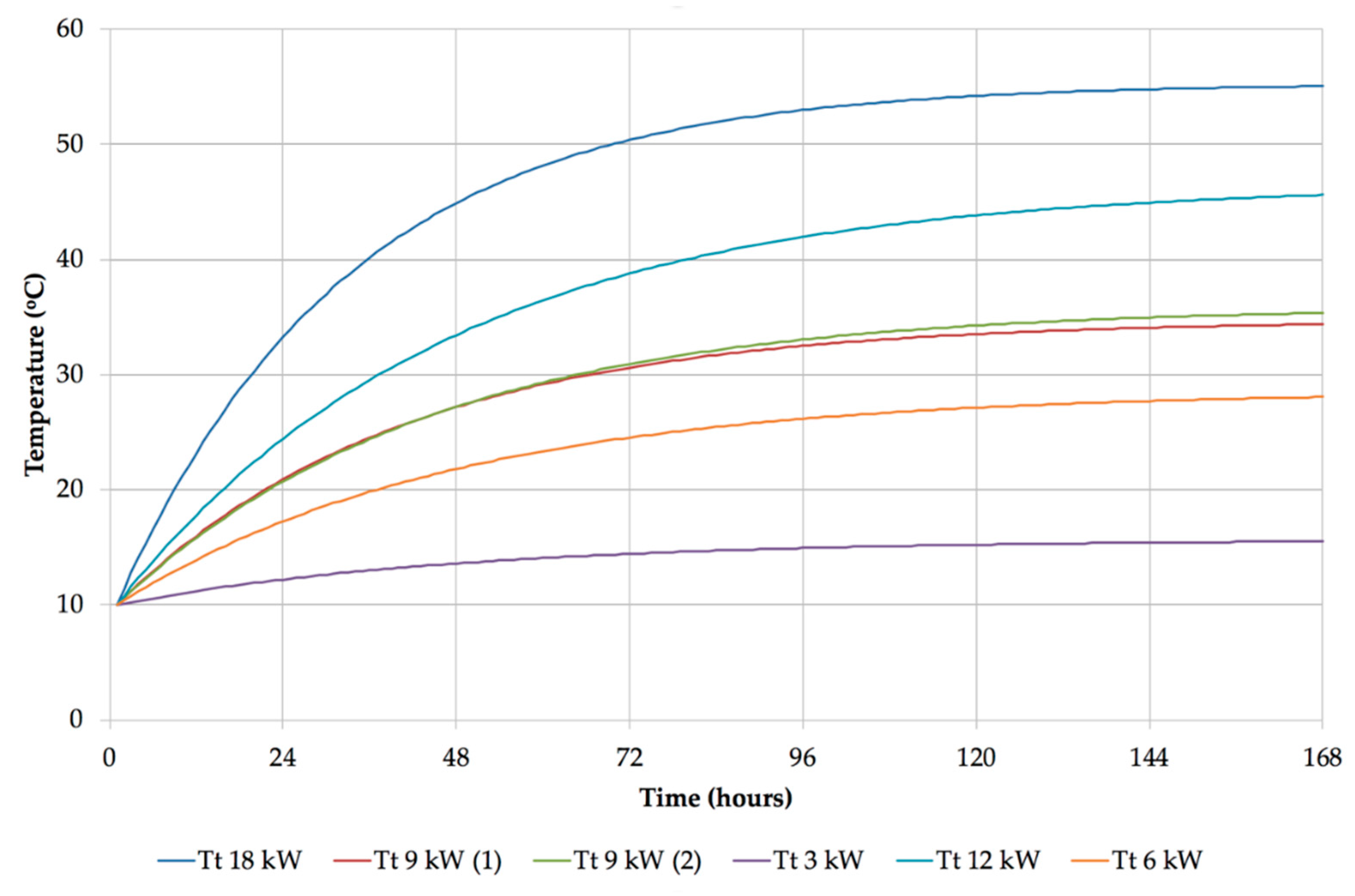
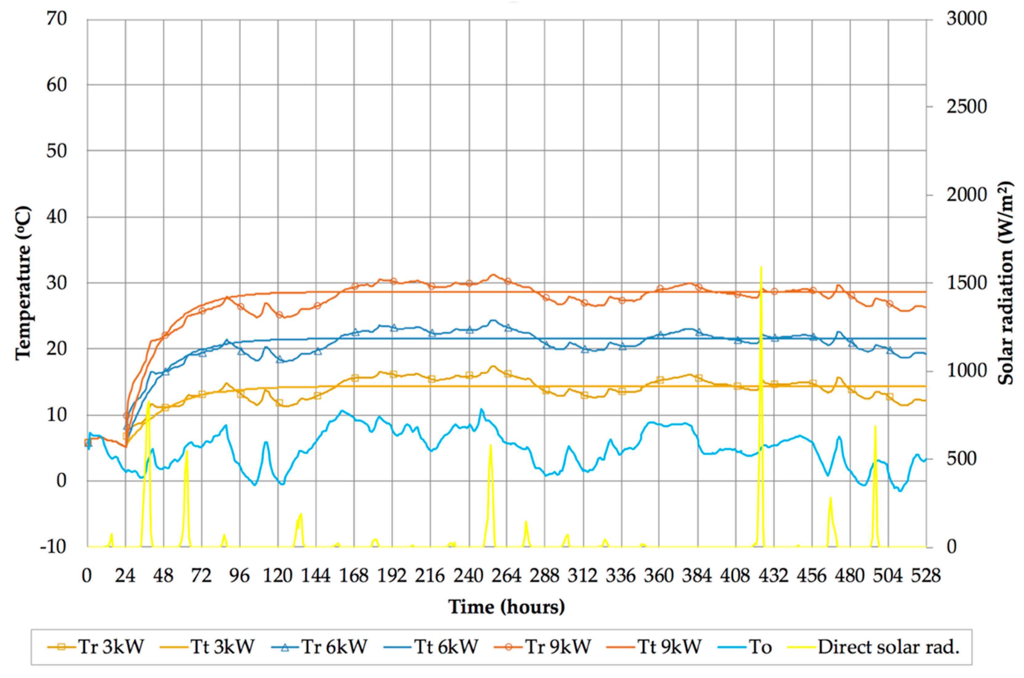
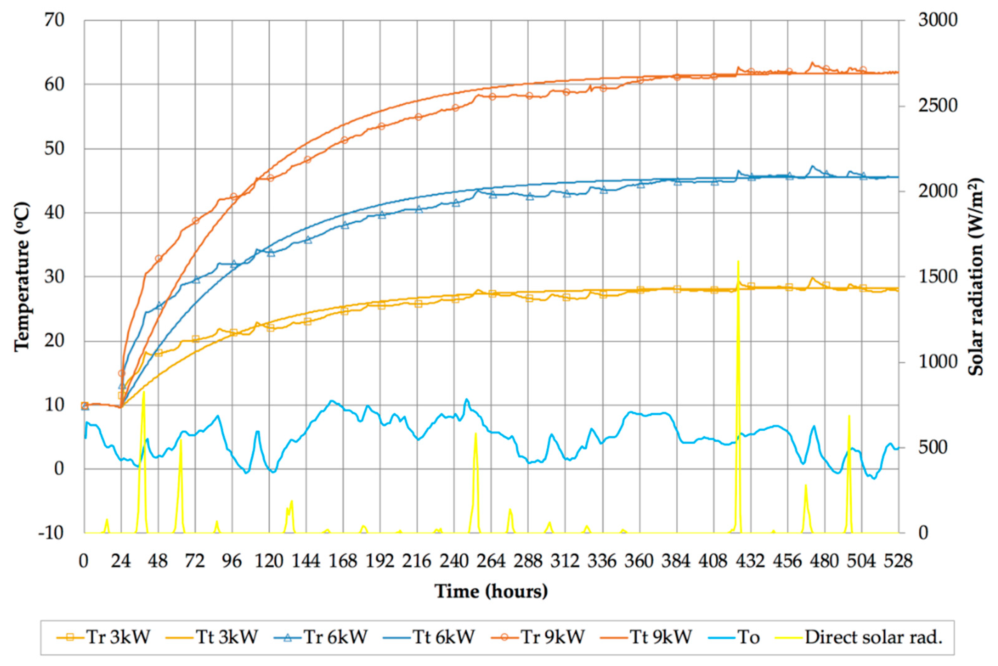
The results of simulations before and after the retrofit are shown in
Figure 12 and
Figure 13, respectively. In both figures, the simulation results are represented with slightly fluctuating curves, and the curve-fitting results are represented with smooth curves. Both simulation results and curve fitting results are represented with the same color for each of the different heating rate inputs. In all simulated tests, the internal heat gains from people, lights, and appliances were set to zero, so that the only other influences on the building temperature were from external air temperature and solar radiation, both shown in these two figures. The scales of horizontal and vertical axes in these figures were kept identical for ease of comparison between the pre-retrofit and post-retrofit simulations.
As can be seen from the pre-retrofit simulations (
Figure 12), the models reached relative steady state within four days after the heating was switched on. This steady state is referred to as “relative” due to the internal temperature fluctuations caused by external air temperature and solar radiation.
In the case of the post-retrofit simulations, the relative steady state was reached only after 14 days, demonstrating a much slower response to heat input in comparison with the pre-retrofit case.
The physics properties obtained from the curve fitting and related calculations in both series of dynamic heating tests are shown in
Table 9.
Therefore, the results of the tests can be expressed as follows:
| Before retrofit: | tc = 21.93 ± 2.65 h
HLC = 328.70 ± 33.05 W/K
C = 25.64 ± 0.38 MJ/K | | After retrofit: | tc = 78.39 ± 1.40 h
HLC = 147.32 ± 12.52 W/K
C = 41.59 ± 3.82 MJ/K |
As can be seen from the results in
Table 9, there was a significant change of building physics parameters through the process of retrofit. The time constant increased 3.57 times to just over 78 h, the heat loss coefficient reduced by a factor of 0.45 to ~147 W/K, and the effective thermal capacitance increased by a factor of 1.62 to just over 41 MJ/K. The overall U-value, which includes the combined effect of all building thermal elements, reduced by the same factor of 0.45 as the heat loss coefficient to 0.69 W/m
2K.
As explained in the
Section 2, the time constant
tc is obtained by curve-fitting to the test results. It is therefore encouraging to see that in both cases, and especially after the retrofit, the standard deviation was low, indicating high accuracy of the results.
But how do the results of dynamic heating tests compare with theoretical calculations of the heat loss coefficient before and after the retrofit? For comparison, the results are shown in
Table 10, side by side with the results of simulated dynamic heating tests.
As can be seen from
Table 10, the theoretical post-retrofit heat loss coefficient falls outside of the range of the heat loss coefficients obtained from the simulations of dynamic heating tests. The discrepancy between the values obtained from simulated dynamic tests and theoretical values is on average 50% after the retrofit, and potentially exceeding 60%.
5. Discussion
Despite of the two sets of dynamic heating tests, physical and simulated, being carried out on different buildings, the average discrepancies of 48% and 50%, and the extreme discrepancies of 62% and 63%, were fairly consistent between the two methods, as shown in
Table 5 and
Table 10.
It was originally intended for simulated dynamic heating tests to be run with the same scenario of heat inputs as in the physical tests, namely 3, 6, 9, 12, and 18 kW. However, in the simulated case, the result of the 12-kW scenario produced a curve that was not equally spaced in comparison with the 3, 6, and 9 kW curves in
Figure 13. This was attributed to an internal limit in the EnergyPlus model that could not be easily found, and it was decided to limit the analysis of simulated dynamic heating tests in this article to 3, 6, and 9 kW inputs.
Although thermal imaging was carried out on both buildings, the results of such surveys are always qualitative, and do not provide a quantitative scale of difference between theoretical and actual building properties, as is the case with dynamic heating tests.
The results of both physical and simulated dynamic heating tests originated from physical measurements taken either directly during the test, or during the calibration of the simulation model using monitored data. For this reason, there was a measurement error in both cases, and thus the results were expressed as mean value ± standard deviation. Despite this uncertainty of the exact values of building thermal properties, there was a significant discrepancy between theoretical heat loss coefficients and the corresponding results of physical and simulated dynamic heating tests. This suggests that designers use inaccurate information when designing building energy performance using theoretical values of building material properties. This makes a case for introducing a safety margin, by downgrading the theoretical building material properties in design calculations and simulations. The scale of this safety margin could go as high as the discrepancies reported in this article.
In the case of simulated dynamic heating tests, there are also two uncertainties related to the process of calibration of simulation models, based on parametric simulation and multi-objective optimization. First, there is an uncertainty that occurs through the interaction of design parameters in parametric simulations, which could lead to a situation where two radically different sets of parameters reach similar outcomes and similar discrepancies between measured and simulated building performance. Second, there is an uncertainty that occurs in the process of multi-objective optimization, which was in this case carried out using the NSGA-II genetic algorithm [
14] built into the JEA optimization tool [
20]. The algorithm starts from a random population of design parameters and applies genetic operations of cross-over, mutation, and reproduction, moving the “offspring” properties closer to the properties of “parent” combinations of parameters, and selecting offspring according to values of objective functions, in order to improve the accuracy of results. In doing so, there is a small chance that a region of the solution space, representing a particular combination of design parameters that leads to better solutions than those found, could be missed.
The chances of the first type of uncertainty influencing the results is eliminated by a close observation and interpretation of results, and, if required, a re-run based on a changed parameter set. The points along the vertical axis in
Figure 2 are sufficiently far from the minimum, so there is no risk of two points close to each other being the result of a radically different set of design parameters, and thus there was no need for parameter changes or re-runs.
The chances of the second type of uncertainty influencing the results are minimized by ensuring a sufficiently small step of each parameter in parametric simulations. The JEA interactive optimization engine used for this purpose first starts with a coarse mesh of parameter combinations and progressively introduces finer meshes in sub-regions of this space [
20].
Finally, it is worth noting a differentiation between the terms of building thermal properties and building physics properties used in this article. “Building thermal properties” refers to steady-state properties relating to and influencing the overall heat loss coefficient HLC. “Building physics properties” are an extension of building thermal properties, and relate to parameters that describe dynamics of heat transfer, such as time constant tc and effective thermal capacitance C.
6. Conclusions
This article investigated the ways of improving building energy efficiency through measurement of building physics properties using dynamic heating tests. The research was initiated in response to a practical question of how to address the risk of U-values being higher than in manufacturers’ specifications, and thus potentially causing long-term and large-scale underperformance of buildings.
A method of measuring building physics properties was developed on the basis of a physical dynamic heating test on a real building and a on the basis of a simulated dynamic heating test with a calibrated model of a retrofitted building. The former is suitable for unoccupied buildings where the duration of the test lasts several days in the case of stable weather, or several weeks in the case of changing weather, and where it would not cause inconvenience of keeping the building unoccupied during that period. The latter is suitable for occupied buildings that have undergone deep energy retrofit and are monitored over a sufficiently long period before and after the retrofit.
In comparison with co-heating tests, which are used to measure the overall heat loss coefficient of the building, the dynamic heating tests provide two more building physics parameters: the time constant and the effective thermal capacitance.
The parameters obtained from the dynamic heating test enable the creation of a simplified but accurate simulation model expressed with Equation (3). The simplicity of this model opens up opportunities for machine learning and predictive control in microprocessor applications.
Both types of tests, actual and simulated, revealed significant discrepancies with theoretically calculated heat loss coefficients for two different buildings. Discrepancies were as high as 62% in the case of the physical test, and up to 63% in the case of the simulated test, with average discrepancies being 48% and 50% in the two respective cases. The consistency between physical and simulated tests is encouraging, as it confirms the usability of the simulated tests as a less-invasive alternative in comparison with the physical tests.
The discrepancies between measured and theoretical values arise from the differences between the in-use context and the laboratory context from where the respective information on material properties originated. The scale of these discrepancies makes a case for using a safety margin in design calculations and simulations, and such a safety margin could be as high as the discrepancies reported in this article. Whilst other sources report large discrepancies between measured and theoretical values of the overall heat loss coefficient [
6,
7,
12], none of these sources question the validity of theoretical material properties reported in technical reference tables.
The simulated dynamic heating test using the calibrated simulation model is a tool for establishing the characteristics of the existing building before the retrofit, and for establishing the quality of the retrofit after completion. The application of this method provides a mechanism for ensuring that the risk of higher U-values in the completed building, in comparison with the values quoted in manufacturers’ specifications, is properly addressed and eliminated.
These results make a case for a systematic review of the published material properties used in building design, in comparison with properties of the same materials in buildings in use.
The application of safety margins in respect to building material properties, and the proposed systematic review of published building material properties, will contribute to improvements in building energy efficiency at a significant scale.


