Evaluation of Cyclic Gas Injection in Enhanced Recovery from Unconventional Light Oil Reservoirs: Effect of Gas Type and Fracture Spacing

Abstract

Production from ultra-low permeability shale plays requires advanced technologies such as horizontal wells with multistage hydraulic fracturing treatment. In this study, a cyclic gas injection method with two pumping schedules is introduced as an enhanced oil recovery (EOR) method. Fracture spacing and type of injection gas in a horizontal well from the Bakken formation are analyzed through numerical simulations. The economic profitability and reservoir performance are also investigated. Rate transient analysis is used to anticipate hydraulic fracture and effective fracture permeability. Different fracture spacings are selected as the major determinant factor in generating an effective reservoir contact area. Compositional simulations are conducted to model incremental oil recovery after cyclic injection of three gases (ethane, CO₂, and natural gas). Economic indicators of net present value (NPV), internal rate of return (IRR) and oil recovery factor are compared to determine the best alternative among the proposed investment scenarios. Current market and a certain time-frame (2015–2035) are used to assess the investment viability of unconventional oil plays. Cyclical injection of ethane and CO₂, remarkably improved oil recovery from the Bakken example. Natural gas injection however, led to inferior results and in terms of investment, may not guarantee the long-term success. Some scenarios are identified as profitable for high oil-API but do not achieve positive outcomes from lower oil specific gravities. The results from this study highlight the impact of fracture spacing in incremental oil recovery. Producing a majority of the cumulative oil during the first years makes most of the scenarios viable only for short terms. To maintain the long-term cost-effectiveness, performing cyclic gas injection through hydraulic fractures is recommended. Cycle sizes directly impact the propagation of injectant and the extent of the drainage area. Increasing the number of fracking stages can be an alternative strategy to gas injection in reservoirs with lower oil-API.

1. Introduction

Bakken, an enormous liquid-rich shale resource and its adjoining formation of Three Forks, extending from North Dakota, Montana, and South Dakota in the United States, to Saskatchewan and Manitoba in Canada, has made strong contributions to oil production in North America. According to the 2013 United States Geological Survey (USGS) project reports, there are 7.4 billion barrels of unrecovered oil that can be produced from the Bakken and Three Forks formations [1]. The U.S Energy Information Administration (EIA) also estimates that the Canadian portion of the Bakken reservoir contains 1.6 billion barrels of oil and 2.2 trillion cubic feet of natural gas [2]. Unconventional reservoirs are difficult to extract due to their restrictive economics and substantial needs for special completion techniques.

Extremely low permeability in unconventional reservoirs prevents oil from flowing naturally into the wellbore. The ultra-low (micro- to nano-Darcy) matrix permeability makes the aforementioned resources geologically unfavorable for recovery. In contrast, the low viscosity and high compressibility of hydrocarbon fluids make them viable potential options for oil production.

The advents of innovations in horizontal drilling and hydraulic fracturing has led the industry to be able to access significant amounts of hydrocarbons in the United States, which were previously considered as unattainable resources. Hydraulic fracturing is the high-pressure injection of a fracking fluid (water, chemical additives to control water viscosity, and proppants) into a horizontal well, at predetermined distances. The pressure creates fractures, which are kept open by proppants providing conductive paths for fluid flow [3]. Hydraulic fracking has provided massively enhanced production in the United States. According to the EIA drilling productivity report for tight oil, total production from the Bakken region has shown a steady growth since 2009 and reached from 200,000 to 1,200,000 barrels per day in 2018 because of the mentioned technologies [4].

However, unconventional oil extraction utilizing fracking methods is accompanied by economic and sometimes technical challenges. In hydraulic fractured wells, by virtue of the conductive paths for fluid flow, high initial production rates and consequently very steep decline rates occur within the early life of the reservoir. Implementing proper EOR methods is required to overcome the quickly flattened recovery and to maintain production levels in unconventional resources.

Secondary and tertiary recovery mechanisms are sought to increase the oil production through pressure maintenance and displacement mechanisms. CO₂ injection, as the second most common EOR method after thermal recoveries for heavy oil [5], has been successfully employed in light to medium oil reservoirs [6,7,8,9,10,11]. However, low permeability and limited injectivity in tight shale reservoirs yield poor gas displacement efficiencies since the injected fluid would take a very long time to spread from the injector towards the producer.

Moreover, because of high degree of heterogeneity in unconventional resources, injectors and producers may not have effective connections for fluid flow. The huff-n-puff method in which the gas injection and oil production are performed in a single well, has made efficient enhanced recovery from tight formations viable. In this method, a gas (e.g., CO₂) is injected into the well for a certain period. After that, the well is shut-in and a soaking time is started. The mechanisms involved in CO₂ EOR consist of an increase in average reservoir pressure, oil swelling, and vaporization of light and medium hydrocarbon components, oil viscosity reduction and enhanced oil mobility [12]. Molecular diffusion of CO₂ in the oil phase also plays a key role in this process. After the soaking period, the well is put into production for a specific time and the whole procedure is repeated. Simulations of the cyclic CO₂-injection method in Bakken have demonstrated incremental [13] oil recoveries between 5% to 20% in multistage hydraulically fractured wells [14]. Results from CO₂ extraction experiments on Upper and Lower Bakken core plugs also indicated that CO₂ diffusion under miscible conditions lowers the oil viscosity and makes the oil extraction from tight cores feasible [15]. Thus, the Bakken formation could be considered as a promising candidate for cyclic CO₂ injection EOR.

In addition, due to huge potential of this EOR method in secure storage of CO₂, much attention has been paid to various designs of CO₂ EOR in previous years. In North America, available and low-cost supplies of CO₂ in addition to vast pipeline networks have led to successful CO₂-EOR projects including the Wasson field in U.S. and Weyburn in Canada [16,17,18].

A successful oil extraction may be affected by many factors such as accessibility of the injection gas, gas price and the investment circumstances. Although promising recovery results from CO₂ injection are obtained, there are some limitations, which are significant controlling factors in EOR projects. Severe corrosion of pipelines, wellhead valves and surface facilities is a challenging issue that usually occurs in CO₂ injection techniques.

Simulation studies have investigated the possibility of using different injection gases for the purpose of shale EOR. Recovery of 6.5% was obtained from natural depletion and 29% incremental oil recovery was observed after cyclic injection of a mixture of 77% C₁, 20% C₂, and 3% C₆ into a hydraulic fractured well in a shale oil reservoir [19]. The obtained oil recovery from CO₂ huff-n-puff into a shale condensate field was slightly higher than methane injection while both greatly outperformed nitrogen injection [20]. Enhanced recovery potential of injecting nitrogen, methane, ethane and CO₂ into shale oil reservoirs has been also investigated through numerical modelling by Li et al. [21]. Ethane has shown great ability in enhancing oil recovery by 15.17%, followed by 9.74% from CO₂ injection, 7.52% from methane injection and 6% from N₂ injection. The lower minimum miscibility pressure (MMP) of CO₂ compared to other gases, including methane and nitrogen, has made it favourable for most of the reservoirs since there is no need for high injection pressure [22].

A profitable cyclic gas injection (CGI)-EOR process is reliant on the availability of sources of the injection gas. In the fields where the available low-cost natural CO₂ resource is not sufficient and other sources of CO₂ such as coal-fired power plants are not economically profitable, miscible or immiscible hydrocarbon gas injection is an alternative technique. In our previous study, we have investigated various uncertainties incorporated in a cyclic CO₂ injection project in the Bakken formation [23]. An experimental design method coupled with numerical modelling were used to introduce the parameters controlling hydrocarbon recovery factor, CO₂ utilization factor, and CO₂ retention factor. Hydraulic fracture half length, fracture spacing, rock permeability, formation porosity, injection pressure, start time of injection and pay zone thickness are the parameters affecting the project’s profits. Different studies also proposed useful methods and algorithms of phase field model for fracture in poroelastic media [24]. The economic profitability and viability of recovery enhancement by hydrocarbon gas injection have been widely investigated and confirmed through simulation studies as well as field operations. Natural gas, methane enriched with C₂, C₃, C₄ or mixtures of CO₂ with C₁, C₂, C₃ are examples of injectants used in EOR projects including North Slope and Prudhoe Bay field [25]. In the latter, CO₂ acts as a carrier gas and miscibility is achieved between oil and C₃ and C₄. The reported West Sak oil (18.5° API) viscosity reduction by ethane was effectively higher than CO₂, followed by C₁ [26]. In another study on West Sak crude oil, miscibility of ethane was observed in lower pressures of around 600 psi while CO₂ miscibility was not achieved even at 6,600 psi [27].

The higher critical pressure of CO₂ compared with ethane, increases its liquefaction pressure. Hence, achievement of liquid state of CO₂ under reservoir conditions (to make it miscible with crude oil) requires higher injection pressure. The non-corrosiveness of ethane and natural gas also minimizes the damage coming from CO₂ acidity and consequent corrosion problems [28]. Moreover, the lower miscibility of hydrocarbon gases in water compared with CO₂, reduces the possibility of gas solution trapping in reservoir brine and consequently a higher gas utilization factor.

However, the relatively higher price of ethane and natural gas compared with CO₂ necessitates further economic analysis to see if utilizing hydrocarbon gases instead of CO₂ can lead to economically sound projects [29,30]. Therefore, it is vital to examine the potential of other injection gases in incremental oil recovery. To do that, accurate field scale simulation is required in order to evaluate the reservoir performance after cyclic gas injection EOR technique using different gases. In this study, using an integrated analytical-numerical method, a reservoir dynamic model is constructed. We designed a CO₂-EOR scheme based on the fixed and growing-cycle sizes of gas injection and oil production. Then an economical decision-based approach is followed to study the effect of stage numbers, gas type and injection schedule on the EOR project economics.

The objective of this study is to deploy different cyclic gas injection scenarios with various fracture spacings to evaluate the potential of different designs of CGI for EOR in the Bakken formation. First, reservoir properties are estimated using analytical modelling. The compositional reservoir dynamic model is then constructed using CMG-GEM software. After history matching, production forecasting is performed in different scenarios to be able to choose the best scenario from both the economical and technical points of view. Two schemes of cyclic gas injection with fixed and growing cycle size are introduced to improve the lateral continuity of injected gas at various fracture spacing. Three injection gases—CO₂, ethane (C₂H₆) and natural gas (NG, a mixture of 75% methane and 25% ethane)—are utilized in our the model. The current study will strive to optimize the asset value for the operators, investors and decision makers by identifying the technically and economically optimum opportunities to maximize production and recovery from other unconventional reservoirs with similar properties.

Four main scenarios proposed in this study are natural depletion, CO₂ injection, ethane injection and natural gas injection. Each scenario uses currently available gas price and oil price data from 2014 through 2019 and forecast data since 2019 to 2035. To examine how the variations in fracking costs, oil price and gas price will affect the ultimate cash flow, a sensitivity analysis is conducted.

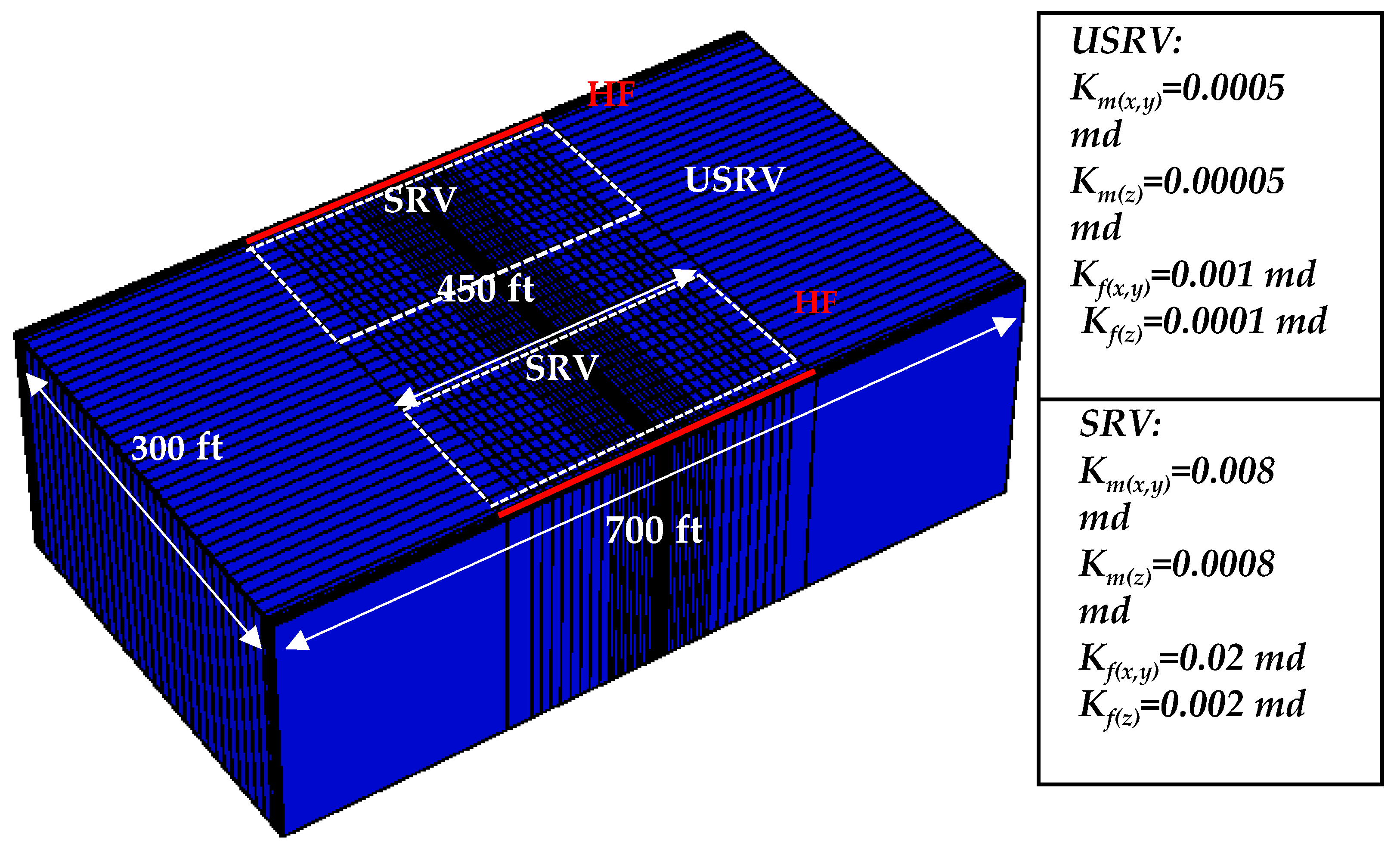
2. Model Construction

Details of rate transient analysis (RTA) calculations are described in our previous work [31]. The calculated hydraulic fracture permeability (10.8 md) and effective fracture permeability (0.02 md) obtained from an analytical model based on flow regimes in horizontal wellbores are used as an initial estimate for history matching in the numerical model. We use production data from the Bakken well to construct a numerical reservoir model. A dual porosity medium defines the natural fractures. Local grid refinement (LGR) is applied in I and J directions within the matrix and fracture blocks near the hydraulic fractures. Hydraulic fracture blocks width (W_hf) is set to 1 ft. Length of stimulated reservoir volume (SRV) is set equal to fracture length of 450 ft and SRV width equals fracture spacing of 300 ft. Effective fracture permeability kf_eff of 0.002 mD and matrix permeability k_meff of 0.0008 mD are found through history matching. SRV and USRV properties of reservoir and fracture are listed in Figure 1. The detailed procedure and results of history matching are reported in our previous publication [32].

2.1. Design of Cyclic Gas Injection

The main mechanism of oil mobilization in unconventional tight resources is known as molecular diffusion of injection gas in oil phase. Miscibility is achieved through multiple contacts and mass transfer between injection gases and crude oil components through vaporization/condensation. Reduced IFT between oil and injection gas leads to oil swelling and viscosity reduction which are the main mechanisms of gas injection EOR [33]. Injection pressures of 5000 psi are used to achieve miscibility.

The molecular diffusion coefficients of CO₂, ethane and natural gas used in this model are set to 5.5 × 10⁻⁴, 4 × 10⁻⁴ and 6 × 10⁻⁴ cm²/s, respectively [13,14]. As mentioned, in the field scale studies of cyclic gas injection process, normally the operation continues for a certain number of fixed-size cycles. However, in our simulation, we investigate and impose proper constraints to adopt a varying cycle size design as outlined below. Fracture spacing is an important factor which defines the extent of drainage area and the potential for improved oil recovery.

In tight formation developments, in addition to recovery forecasts, the environmental effects and drilling costs of fracking stages must be taken into account. Reservoir contact area can be improved by identifying proper fracture spacing as well as pumping schedules. Stimulated area and effective fracture half-length in horizontal wells determine the extent of injection gas in the reservoir. In most field scale simulations constant duration for both injection and production cycles are used for cyclic-injection process design. However, in this study, we adopted a variable cycle size where the injection cycle are continuously increased to fill the previously depleted reservoir volumes. To obtain larger lateral gas continuity between hydraulic fractures longer cycles are utilized in wider fracture spacing. The injection and production lengths for each cycle are selected depending on the fracture spacing. For wider spacings, cycle sizes are extended while for narrow spacing smaller cycles are used.

In the fixed cycle scheme, the well produces under the natural depletion for 150 months and then a cyclic gas injection scheme is applied for total of 270 months. In the later cycles, larger volumes of the reservoir are being drained and more gas is needed to fill the depleted sections. Hence, in an extended cycle scheme the injection duration is increased at the constant injection pressure in order to provide larger volume of solvent. Production cycles are also extended at later cycles as the drainage area in the reservoir is extended. In this design, the soaking intervals are kept constant and injection and production cycle sizes are growing as listed in

Table 1. Injection and Production Cycle Sizes.

Stage#	Fracture Spacing (ft)	Injection Cycle Length (Days)							Production Cycle Length (Days)
		1	2	3	4	5	6	7	1	2	3	4	5	6
n = 10	900	40	40	48	56	64	64	64	112	120	128	144	160	168
n = 15	600	26	26	32	37	42	42	42	74	80	85	96	106	112
n = 20	450	20	20	24	28	32	32	32	56	60	64	72	80	84
n = 25	360	16	16	19	22	25	25	25	44	48	51	57	64	67
n = 30	300	13	13	16	18	21	21	21	37	40	42	48	53	56
n = 35	257	11	11	13	16	18	18	18	32	34	36	41	45	48
n = 40	225	10	10	12	14	16	16	16	28	30	32	36	40	42

.

Results from oil production simulation of each fracture spacing just before start of CGI are shown in Figure 2. The difference in produced oil disappears for more than n = 20 hydraulic fracture stages. At the same time one can conclude that 15 fracking stages giving RF = 16.56% is not significantly different from higher stage numbers of 20 to 40 with recoveries of 17.27% to 17.39%, respectively. However, 10 fracking stages leads to the least recovery of 13.68% due to insufficient drainage volume around each hydraulic fracture.

Figure 3 and Figure 4 show the average reservoir pressure (dashed lines) and oil recovery factor (solid lines) during CGI in both fixed and growing cycle sizes for n = 10 and n = 35. As shown, the extended cycles are capable of maintaining the average reservoir pressure effectively higher than that obtained from fixed cycles. This allows for extension of the injection zone and more efficient diffusion between CO₂ and oil. As a result, the oil recovery factor in FS = 10 is improved from 15.8% to 17.7% and in FS = 35 it is slightly changed from 28.6% to 29.09%. The more number of fracture stages, the less changes between two injection schedules are observed. The reason is more effective depletion of SRV in any type of injection. However, with less number of fractures, extended cycles lead to higher oil recovery. This method can provide enough time for the injected gas to penetrate into the reservoir and contact the in-situ oil.

2.2. Effect of Injection Gas

Measured MMPs for Bakken crude oil sample (with 38 API gravity) and pure CO₂, methane and ethane are reported in an experimental study by Hawthorne et al. [34]. Under measurement conditions of 110 °C, the MMPs of oil and ethane, CO₂ and a mixture of 74.1% methane and 25.9% ethane were 1359, 2520 and 3165 psi, respectively. Figure 5 and Figure 6 compare original oil in place composition, oil composition after natural depletion (ND) and oil composition after CGI by CO₂, C₂ and NG. The plots clearly demonstrate the ability of ethane in mobilizing an entire range of hydrocarbon molecular weights while showing that CO₂ preferentially extracts lighter hydrocarbon components [35]. The results from NG injection are fairly comparable with the natural depletion mechanism.

The effect of injection gas on oil recovery can be explained using the definition of MMP at which the IFT reaches zero [34]. Figure 7 and Figure 8 plot the IFT changes in a single grid block versus time in all three scenarios of CGI for both API gravities. As it can be seen, with the emergence of solution gas as a result of a sharp pressure drop below the bubble point pressure, IFT increases from zero to 7 dyne/cm in a light oil sample. After the CGI is started, at each injection cycle, the IFT dropped to around zero due to increase in pressure and occurrence of miscibility between oil and injection gas. However, IFT between oil and methane is slightly higher than zero, showing that a full miscibility is not achievable for this gas. As the production cycle starts, the pressure drops and IFT immediately increases which demonstrates the existence of two-phase flow. In the scenario of cyclic methane injection, IFT reaches to the highest value compared with the two other gases, that confirms its incomplete miscibility with oil. This results in a larger portion of dissolved gas coming out of solution and leads to relatively higher IFT. Overall, CO₂ acts better than methane in lowering the IFT and ethane outperforms the two other gases. In a 31° API oil sample, the same trend is observed. However, the range of IFT is relatively higher due to existence of heavier molecular weight pseudocomponents.

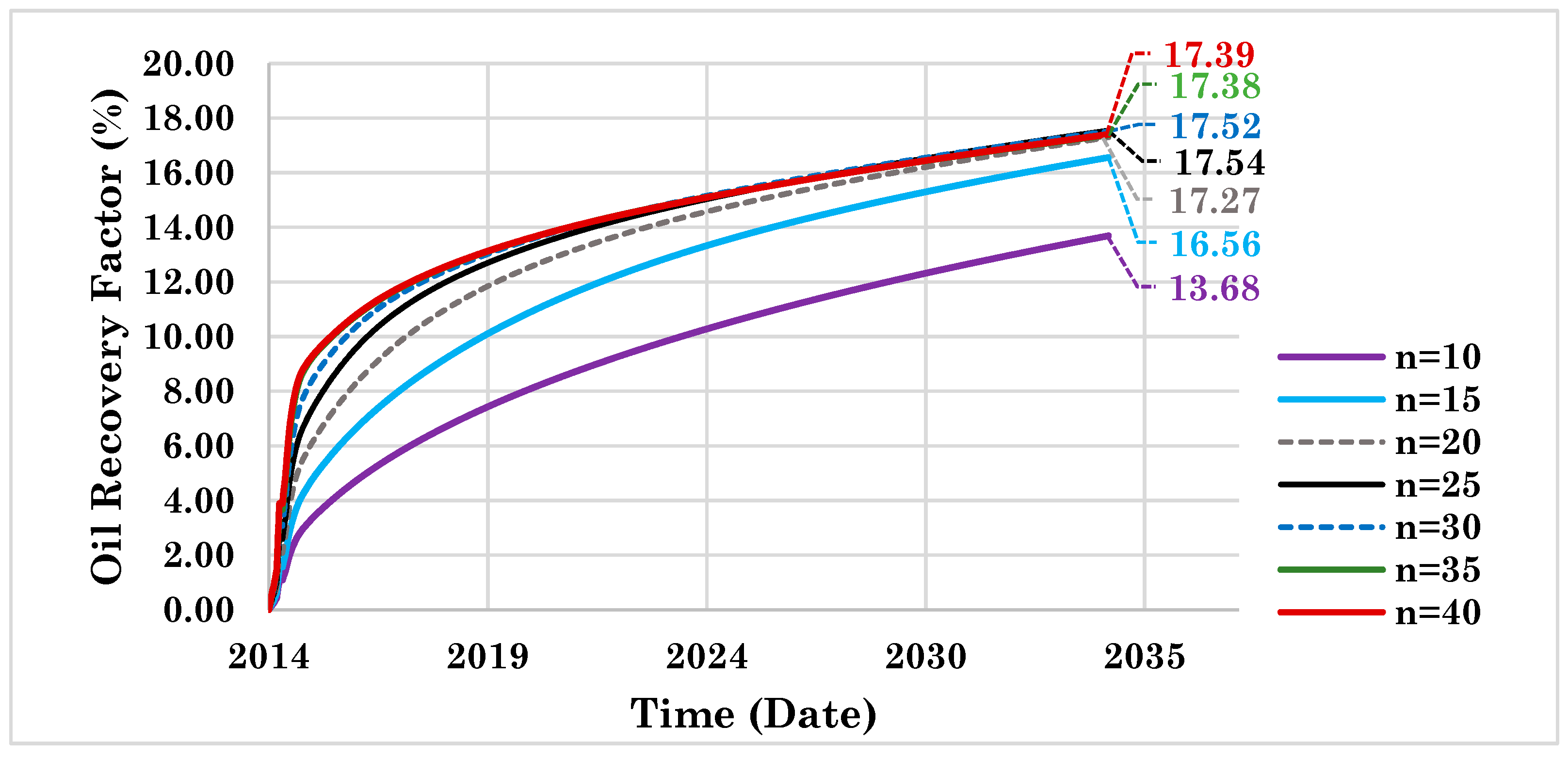
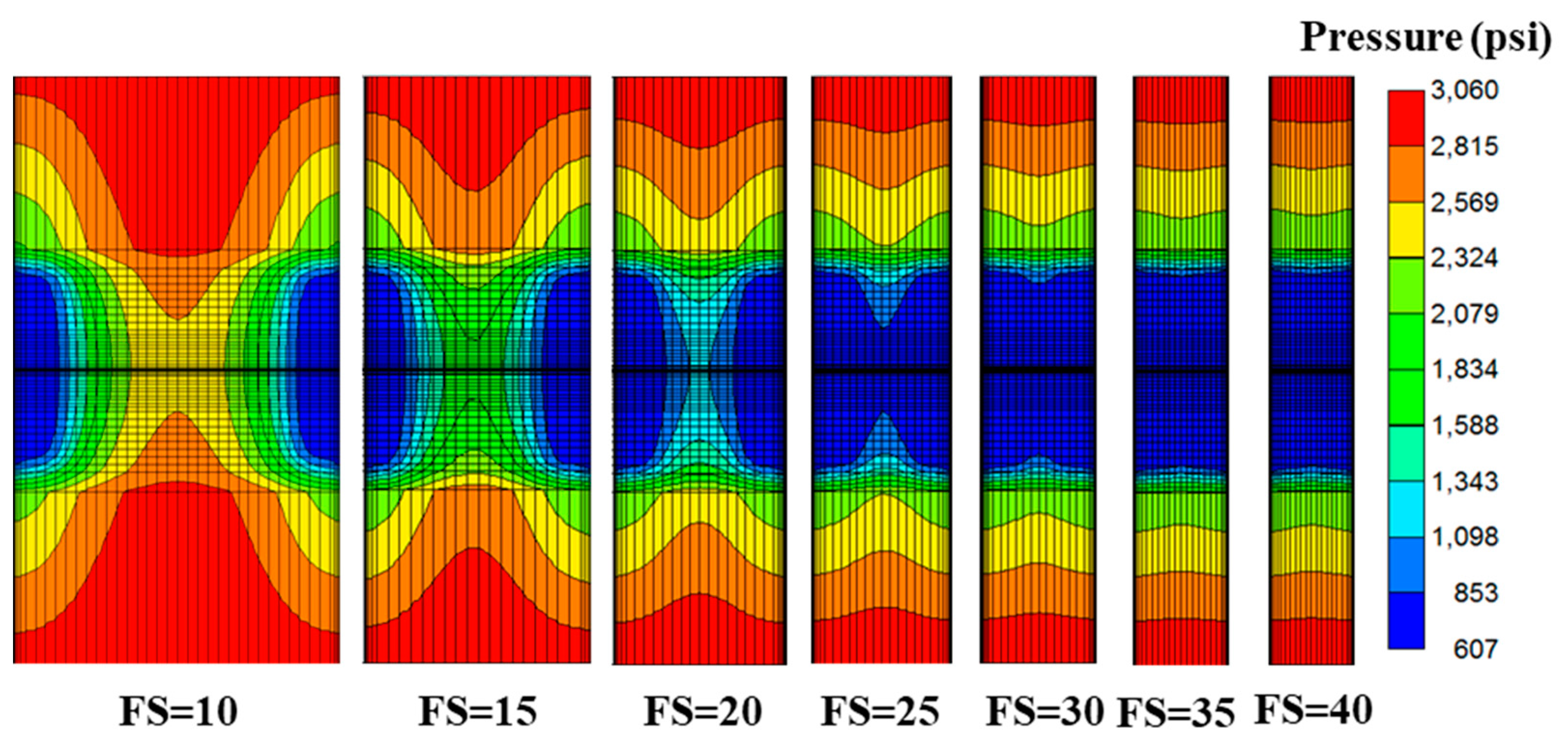
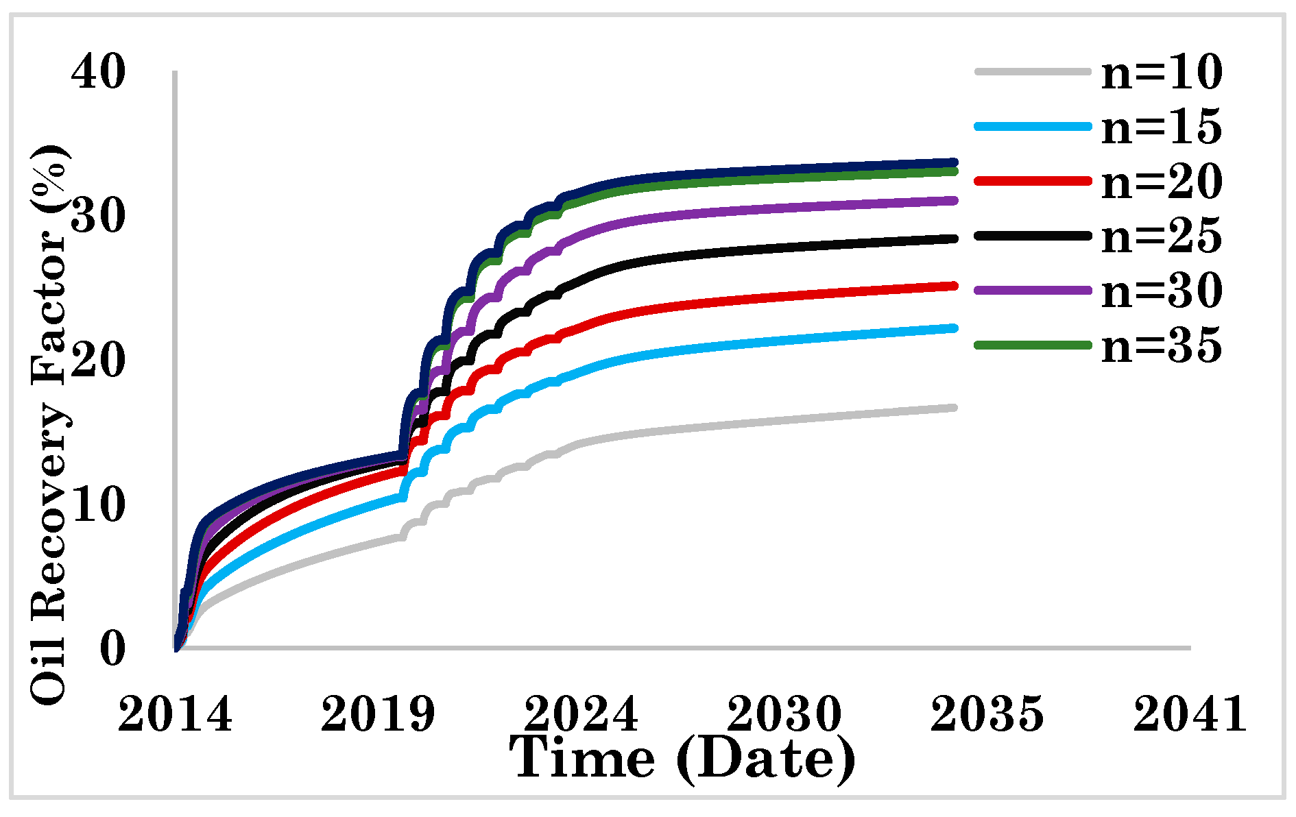
2.3. Effect of Gas Type Coupled with Fracture Spacing

This section is focused on identifying an optimum fracture spacing for each scenario that gives the higher oil production regardless of any other factor. The contour plots of average reservoir pressure after one year of natural depletion between two adjacent fracture stages are shown in Figure 9. The figure shows that quick pressure depletion occurs mostly within the SRV region (K_m = 0.008 md and K_f = 0.02 md) due to conductive fracture network, while pressure in USRV region (K_m = 0.0005 md and K_f = 0.001 md) remains almost the same as the initial reservoir pressure. This behavior also demonstrates the importance of fracking stimulation operations in unconventional reservoirs. Yet, a large area of the reservoir will remain un-depleted, hence the production ends with a high residual oil saturation. The figure also demonstrates the effect of fracture spacing on reservoir pressure distribution. More number of stages decreases fracture spacing, leading to more uniform pressure depletion. However, in the lowest fracture stage, the area between neighbor fractures will not deplete effectively.

Table 2. Recovery factors from fixed and extended cycles scenarios at three fracture numbers of 10, 15 and 20 during injection of C₂, CO₂ and NG.

Frac #/Scenario	n = 10		n = 15		n = 15
	Fixed	Extended	Fixed	Extended	Fixed	Extended
C2	16.64%	20.27%	22.14%	26.12%	25.07	28.35
CO2	15.50%	17.28%	19.97%	22.4%	21.99	23.83
NG	14.05	15.73	16.82	18.93	17.51	19.64

compares the ultimate recovery factors from various scenarios with the largest fracture spacings (fracture stages = 10, 15 and 20). Recovery factors from each scenario are obtained and the results are shown in Figure 10, Figure 11, Figure 12, Figure 13, Figure 14, Figure 15, Figure 16, Figure 17, Figure 18, Figure 19, Figure 20 and Figure 21 for both high and low oil API gravities. Comparing the ultimate recovery of oil, extended cycles in wide fracture spacings leads to more effective extraction of available reserves compared with fixed-cycle designs. For instance, the extended and fixed cycles of ethane injection respectively give 20.27% and 16.64% from 10 fracture stages and 26.12% and 22.14% from 15 fracture stages. The difference is minimized at higher fracture stage numbers. Extending the CO₂ injection cycles leads to 17.28% and 22.4% RF from 10 and 15 fracking stages while 16.64% and 19.94% RFs are obtained from 10 and 15 fracking stages with fixed cycles.

2.4. Economic Assumptions

Hydraulic fracturing is used to improve the poor flow rate in low permeability shale formations. After drilling the horizontal wellbore and conducting perforations, high-pressure fracking fluid is injected into the well to create fractures within the drainage area. Highly conductive fluid paths expose larger resources and provide more contact areas between reservoir and wellbore which facilitates oil flow into the wellbore. The associated costs of this new technology are higher than conventional completions as a result of longer well laterals, additional operations and materials needed for well fracking. In this completion method, fracking pumps, equipment and required horsepower atone for almost 24% of total cost of U.S. onshore drilling and completion [36]. Proppant as fracking fluid additives, which are used to open up the cracks, make up on average 14% of the total costs. Operator’s tendency is increasing the number of fracture stages to mitigate the effect of sharp decline rate in hydraulic fractured wells. From the simulation results of various fracture spacing values, additional fracking and minimizing the spacing improves the oil production by providing more effective reservoir contact area. However, increasing the number of stages brings additional costs due to enhanced amount of material used as proppant, workovers and high injection rates. In this section, economic analysis is performed to see if the smaller fracture spacing in a fixed lateral length and corresponding higher well performance is capable of offsetting the drilling costs or may lead to higher total cost and unprofitable investment.

In addition to oil price and the nature of reservoir fluid/rock properties, criteria for an economical EOR method consists of various basic operational factors including access to capturing pipelines, installation of recycling plants, corrosion-resistant facilities, gas compression/injection plants and production units. Available gas resources as well as purchase prices are also influential factors in economics of any gas injection process. Although operating expenses depend on many variables including well performance and well location, in the current study, an estimate of total cost for typical Bakken well is used in the analysis and is kept the same for all scenarios. This cost is comprised of three key cost sources of drilling, certain facility configuration/completion and the amount of required material associated with fracking and cyclic gas injection. Average leasing cost of $3MM is used for a Bakken well in 2014. The costs for gas gathering, processing and transportation are not included in our analysis since the mentioned costs depend on the availability of plants and pipelines which may substantially vary in different plays.

Average drilling cost of a typical Bakken well with 8600 ft length including rig rates, drilling fluids, casing and cement costs is estimated around $2.4MM, making up 31% of total well cost. In addition to facilities cost of $0.6MM, completion cost for 25 frack stages is approximately $4.4MM, accounting for almost 63% of total well cost consisting of: completion fluid (including volume of consumed water, chemical additives and gel, and type of fracking fluid), hydraulic fracture pump/equipment and artificial/natural proppants. Costs of injection gas during CGI are assumed based on the most recent EIA report for historical and forecasted prices for CO₂ [37], ethane [38] and natural gas [39]. Crude oil historical and forecasted prices are also obtained from natural energy board [40]. Inflation of 2.8% is considered as increase in oil price per year. Cash flow statements as a useful tool for assessment of oil and gas investments are used to calculate net present values (NPV), internal rate of interest (IRR) and selection of optimum production scenarios. NPV is defined as the difference between sum of the cash inflow present values (PVs) and the sum of cash outflow PVs, calculated as Equation (1) [41]:

$$NPV={\displaystyle \sum }_{n=1}^{n=20}\frac{C_n}{{\left(1+r\right)}^n}-C_0$$

(1)

where C_n is net cash inflow during the period n, C₀ is total initial investment costs, r is discount rate and n is umber of time periods. IRR (Equation (2)) ascertain the discount, which makes the present value of all cash flows (outflow and inflows) equal to zero:

IPR = PV of cash inflow − PV of cash outflows = 0

(2)

The analysis provides information concerning the cash receipts and cash payments. A rate of return of 10% as minimum acceptable discount rate is selected to obtain the equivalent values of future cash flows. The investment period of this study is considered twenty years between 2015 and 2035. Each positive net present value specifies profitable investment, indicating that the projected cash flows from the corresponding scenario is greater than the costs. To calculate net present value of each scenario as of some years prior to 2035 the cumulative NPV is also calculated. Internal rate of return is the discount rate equaling the present value of cash inflows to the initial investment and identifies the overall gain or loss of an investment project. Approximately, at any IRR value higher than 10%, the investment opportunity may be a good one.

3. Economic Analysis Results

In this section, a cash flow is constructed and profitability indicators are calculated. Before conducting cash flow statements, cumulative oil production, cumulative injected gas and cumulative produced gas of each scenario are extracted from our compositional numerical model. It is assumed that 10% of produced gas in each production cycle is re-injected to the reservoir in proceeding injection cycle. Due to variable parameter within the scenarios including fracture spacing, oil price, gas price, and various production performances from CGI (due to variable cycle size and oil gravities) different results are obtained. As it can be seen from the oil recovery plots, due to the specific structure of unconventional fracked reservoirs and highly conductive flow paths, oil recovery is ramped up quickly during the initial year of production. NPV is negative during the development phase (year 0 to 1) and starts to increase immediately after start of natural depletion. It decreases as production continues (year 2 to 7), and experiences a second peak after start of CGI, a quick increment (during production period) and an immediate decrease (during injection period) at each cycle corresponding recovered oil and the costs associated with gas injection, respectively. Decreasing trend of NPV results from flattened plots of oil recovery as cycles proceed which are clearly shown in cumulative NPV plots. Different behavior of NPVs in various scenarios at each fracture spacing is due to different parameters involved such as injection gas price, cycle size and produced oil volume.

NPV and cumulative NPV plots of two scenarios with 30 and 10 fracking stages are shown in Figure 22, Figure 23, Figure 24, Figure 25, Figure 26, Figure 27, Figure 28 and Figure 29. The plots illustrate annual profit of the scenarios for fixed and extended cycles of cyclic CO₂, C₂ and NG injection as well as natural depletion. Extended cycle scenarios have shown more durable NPVs compared with fixed cycle scenarios. This trend can be observed easily in cumulative NPV plots in which extended cycles are always located above the fixed cycle regardless of injection gas type. Oil recovery factor, IRR and cumulative NPV during the reservoir life are summarized in

Table 3. High API and low API Oil recovery factor, IRR and cumulative NPV during the reservoir life for n = 30 and n = 10.

FS/Oil API	Economic Indicator	Fixed-C2	Fixed-CO2	Fixed-NG	Extended-C2	Extended-CO2	Extended-NG	ND
n = 30, 38 API	RF(%)	30.87	28.38	19.79	32.02	29.51	20.42	16.77
	Cum NPV (MM$)	18.55	17	11.35	19.09	17.48	11.64	10.73
	IRR	168.04	169.82	167.6	168.02	169.82	167.61	167.4
n = 30, 31 API	RF(%)	22.27	20.062	13.51	23.05	20.96	13.87	10.03
	Cum NPV (MM$)	14.45	11.18	6.87	11.9	10.61	5.9	5.05
	IRR	82.08	80.44	78.85	82.26	80.34	77.8	77.24
n = 10, 38 API	RF (%)	17.7	16.61	14.05	19.54	17.79	15.73	12.92
	Cum NPV (MM$)	8.36	7.76	6.13	9.15	8.3	6.93	6.04
	IRR	64.04	63.4	61.39	63.91	63.32	62.17	61.04
n = 10, 31 API	RF (%)	10.63	10.63	8.22	13.24	10.06	9.56	6.78
	Cum NPV (MM$)	3.77	3.77	2.83	2.44	4.86	2.98	1.82
	IRR	30.21	27	24.06	29.93	26.46	25.18	21.69

.

3.1. 38° API Oil

Our results demonstrate that fracking additional stages significantly accelerates oil recovery. With 30 fracture stages, NPV increases from $−3.84MM to $8.84MM within the first year of production, while with 10 fracture stages NPV has only reached from $−3.03MM to $3.29MM. It can be seen that more stages are profitable to quickly pay off the costs related to fracking operation and the corresponding additional required material. The second peak in NPV occurs at 8th year of the project, when the CGI process is started. The maximum NPV obtained from 30 stages is $4.08MM, which is much higher than $1.62MM from 10 stage. The case with natural depletion mechanism, has led to recovery factors of 12.92% from 10 stages and 16.77% from 30 stages illustrating that increment in recovery is only marginal with increase in fracking stages and to achieve a profitable project, any type of CGI is recommended.

With comparison of only recovery factors, one may conclude that the scenarios with 10 stages-C₂ (fixed), CO₂ (fixed and extended) and NG (extended) injection (17.7%, 16.61%, 19.54% and 17.79%, respectively) are commensurate with 30 stages-natural depletion (16.77%). However, lower NPV and IRR indicators suggest that although higher recovery is achieved from CGI, more fracking stages and oil production under natural depletion mechanism lead to more attractive economic. The reason is inclusion of injection gas costs into the analysis.

Produced oil and corresponding NPV and IRR values of CGI confirm that maximum oil recovery from all fracture spacings is obtained from cyclic injection of ethane followed by CO₂ and NG. The extended cycles regardless of gas type are capable of improving the recovery compared with fixed cycles. NPV and IRR values compared to cases without EOR mechanism strongly confirms that conducting the CGI can improve the project’s profit.

3.2. 31° API Oil

Thirty fracture stages yield an increment in NPV from $−3.84MM to $5.42MM within the first year of production while 10 fracture stages are capable of increasing NPV from $−3.03MM to $1.87MM. The highest peak in NPV after CGI is from ethane injection followed by CO₂ and NG. Natural depletion from 30 stages leads to 10.03% recovery factor while CGI in 10 stages lead to higher recoveries of 10.63%, 13.24% and 10.06% from C₂ (extended) and CO₂ (extended and fixed) injection respectively. However, again when cost-effectiveness of the mentioned scenarios is evaluated by means of NPV and IRR instead of RF, it clearly can be seen that more fracture stages is more beneficial to the project’s economic rather than CGI technique. Same as the results from 31°API oil, higher recovery and NPVs are gained from extended cycles compared to fixed cycles.

4. Economic Indicators Sensitivity Analysis

In the previous section, the project cash flow was constructed from obtained production, cost and fiscal assumptions. In addition, applied discounted cash flow was used to determine the net present values. To identify the feasible EOR scenarios and the possible alternatives, sensitivity analysis on profits is performed in this section. The cost and schedule for the field developments will form the basis of this economic analysis. Accurately determining the ultimate oil recovery and precise estimate of the costs associated with fracking and CGI, have significant impacts on the benefit or detriment of the EOR project. From spider plot, the economic inputs, which are sensitive to the NPV/IRR and exhibit large influences, can be identified and prioritized. The gas costs and oil price are also variables that change with time. In this section sensitivity analysis are carried out to see how NPV and IRR change with ±30% and ±15% variation in gas cost, oil price and fracking costs. The spider chart of changes in NPV and IRR are shown in Figure 30, Figure 31, Figure 32, Figure 33, Figure 34 and Figure 35, for 31 °API and 38 °API gravities in some scenarios. The most and least sensitive scenarios are shown with black and red curves respectively.

4.1. 38° API Oil

4.2. 31° API Oil

5. Conclusions

CO₂ preferentially mobilizes the lighter oil components and reservoir residual oil becomes heavier with time. The molecular selectivity of CO₂ leads to the retention of intermediate and heavy components in residual oil. Natural gas has higher MMP compared with CO₂ and pure ethane. Because miscibility is achieved quicker than with CO₂ and NG, ethane is capable of effectively mobilizing the light, intermediate and even heavier hydrocarbon components. The poor performance of natural gas is related to incomplete miscibility and inefficient mobilization of crude oil. To observe how the IFT changes in each scenario, one grid block is selected and the IFT trend versus time is plotted for all cases.

Though the volumes of injected solvents are identical for all scenarios, pure ethane has led to highest oil recovery for the same production time and operation conditions. Comparison between three injection gases of C₂, CO₂ and NG, the ethane-EOR results in terms of RF are the most favorable followed by CO₂ and NG.

Constant and extended C₂, CO₂ and NG injection modes are compared along with the primary production recovery. Number of fracture stages is also studied in terms of profitability and are included in economic analysis. By sensitivity analysis of uncertainties on the key field development metrics (ultimate produced oil and costs) and visualizing the results in spider plots the impacts can be ranked. The vertical range generated by each parameter represents the expected range of profits it would produce if the changes in that parameter varies between the minimum and maximum (−30% and +30%).

Result shows that fracking cost and gas price have the minimum influence on project’s economic corresponding to short vertical ranges in NPV and IRR. However, reduction in oil price shows a huge effect and extends the vertical range to more negative NPV values. This reduction is intrinsic in large fracture spacings. In fracture stages more than FS = 20, the NVP and IRR changes becomes minimum.

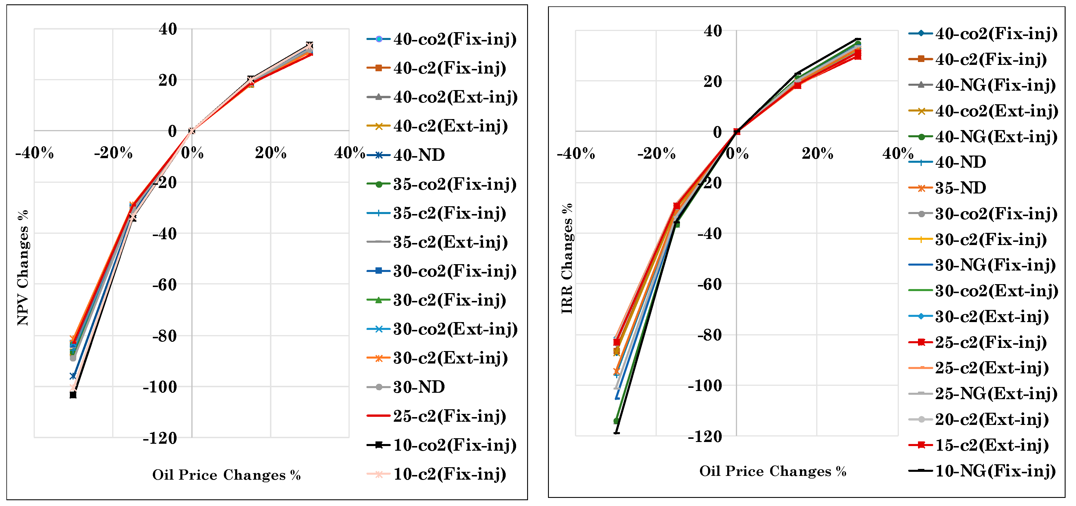
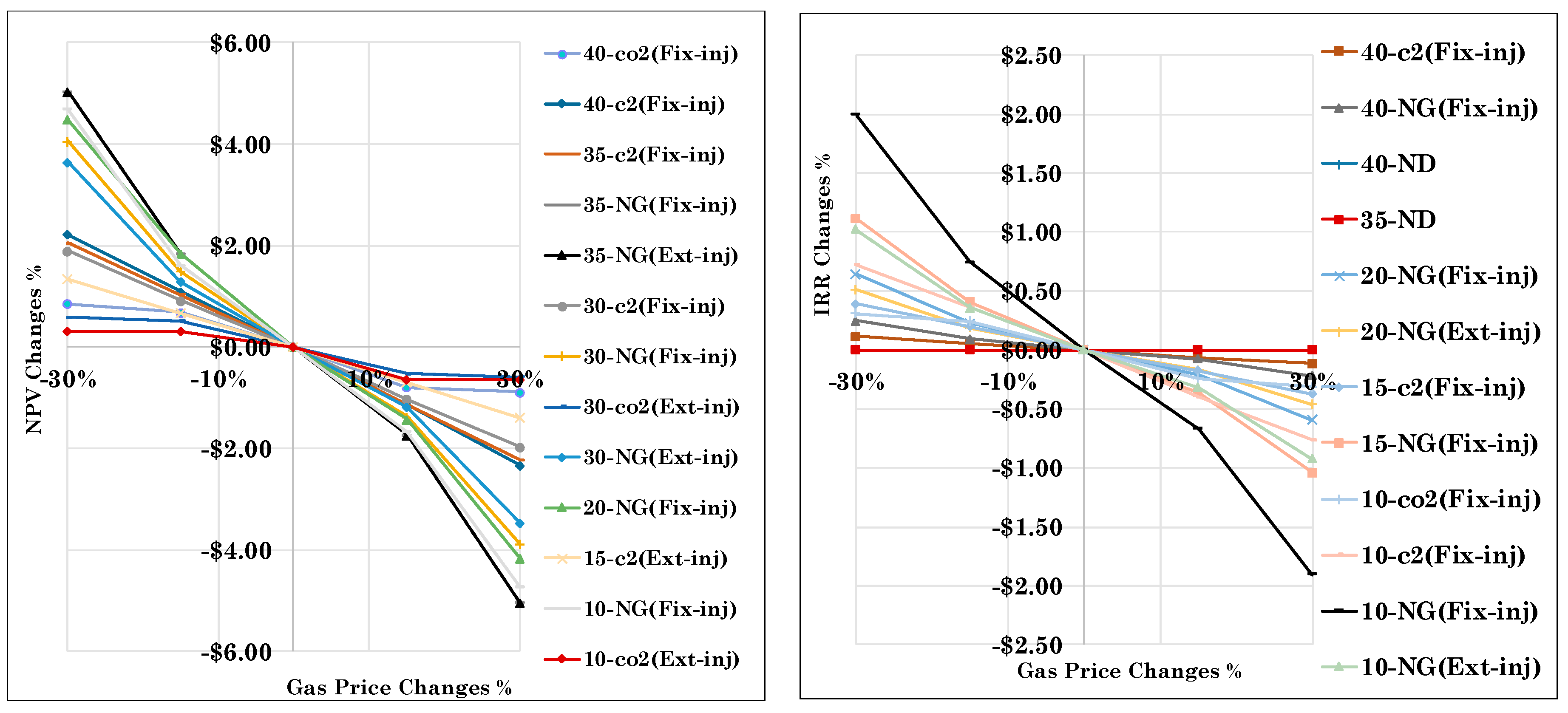
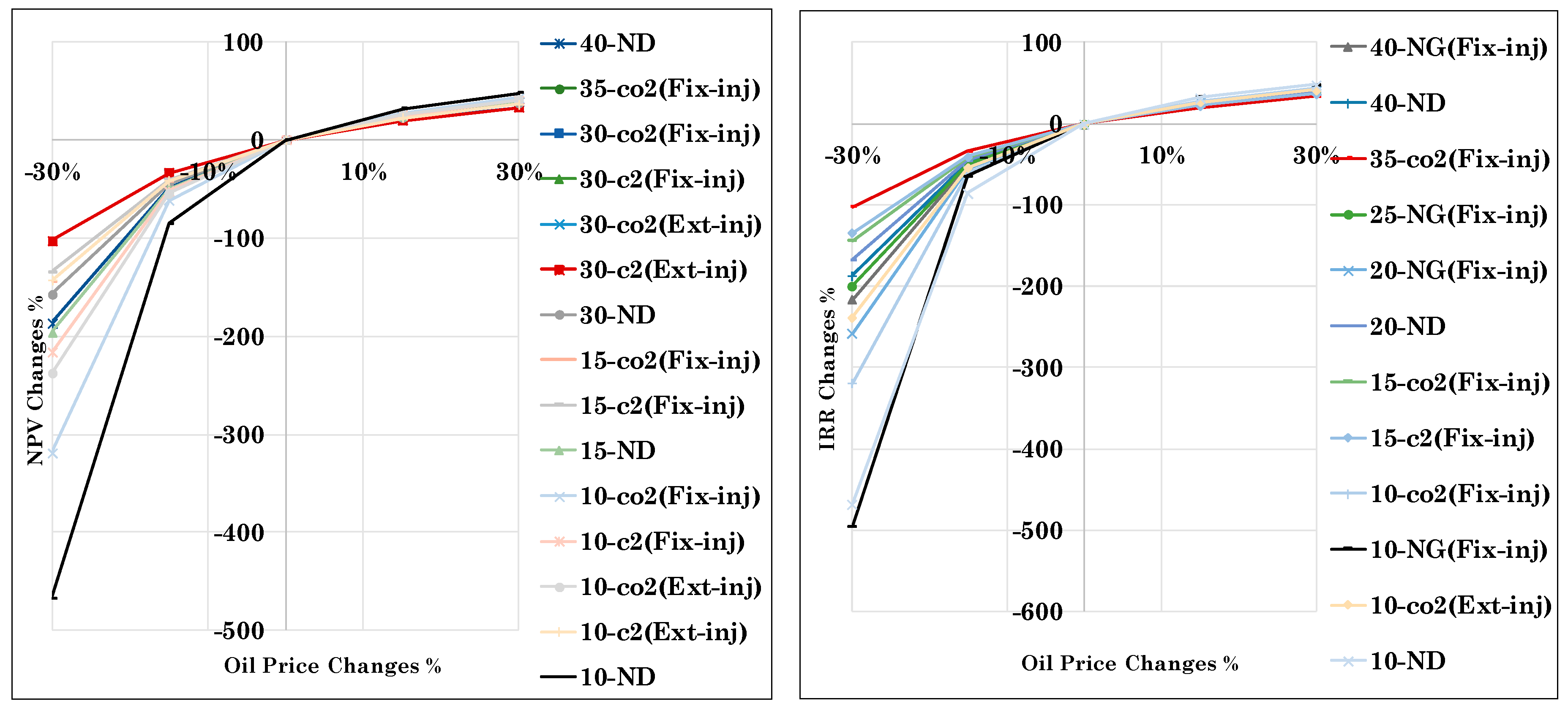
• Amongst the variables, oil price is the most influential factor in project’s NPV and IRR. Oil price decline has a dramatic effect on NPV and IRR and −30% changes leads to 467% decrease in NPV while 30% increment in oil price only results in 48% higher NPV.
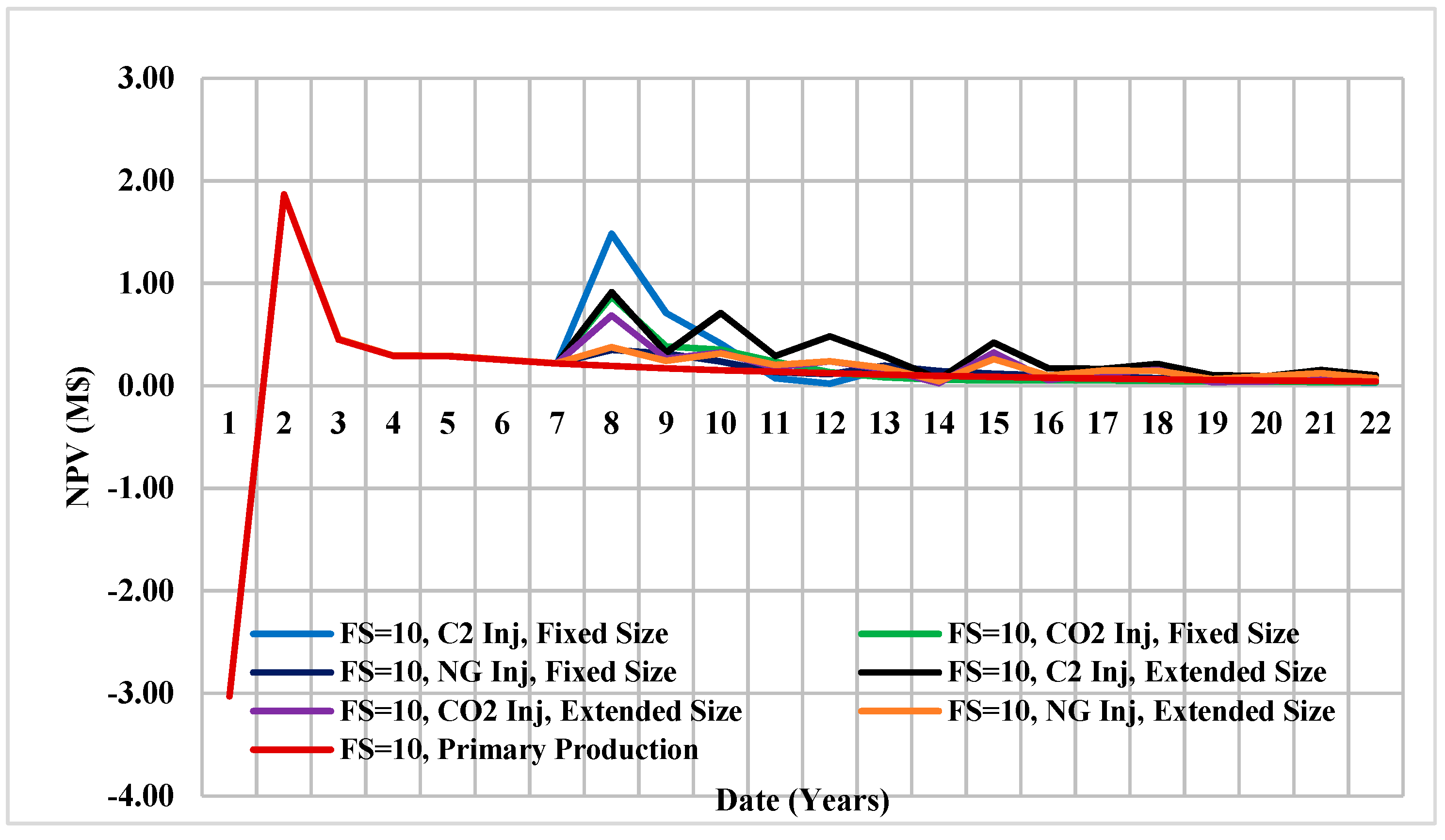
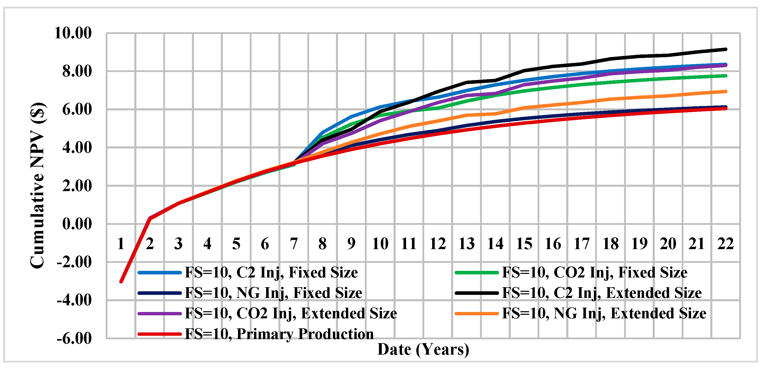
• When the oil price declines by 30% and 15%, cumulative NPV is reduced by −100.24% and −33.39%, meaning that while keeping the rest of the costs constant, 30% decrease in oil price may lead to negative NPV and IRR, making the project uneconomic. This trend is seen in scenarios for FS = 10-C₂ (fixed) and FS = 10-CO₂ (fixed). The scenario of FS = 25-C₂ (fixed) is showing the minimum reduction in NPV. Almost all the scenarios will result in 30%−33% and 19%−20% increment of NPV if the oil price increases by 30% and 15% respectively. Variation in IRR lies between −120% and −80% with 30% decline in oil price and between −28% to −35% with 15% decline in oil price.
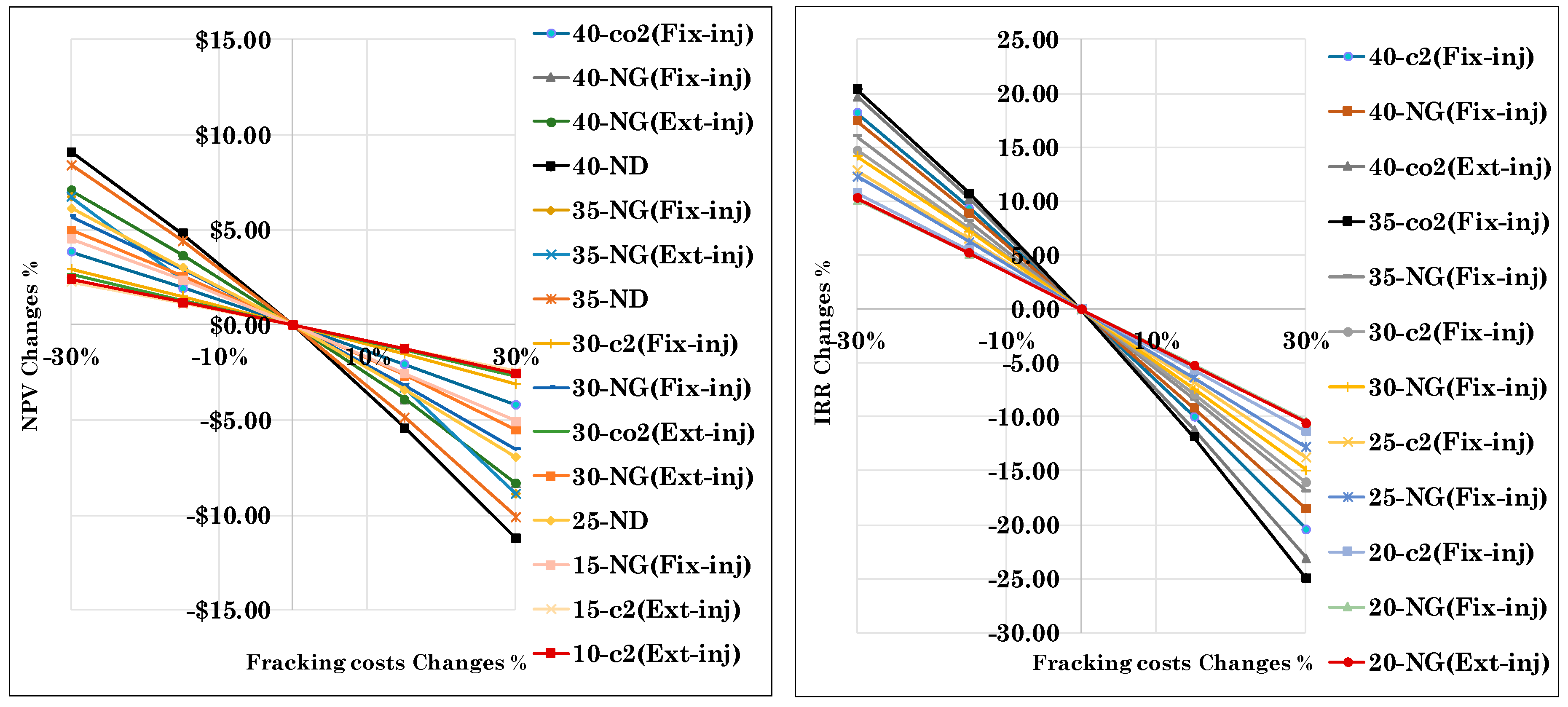
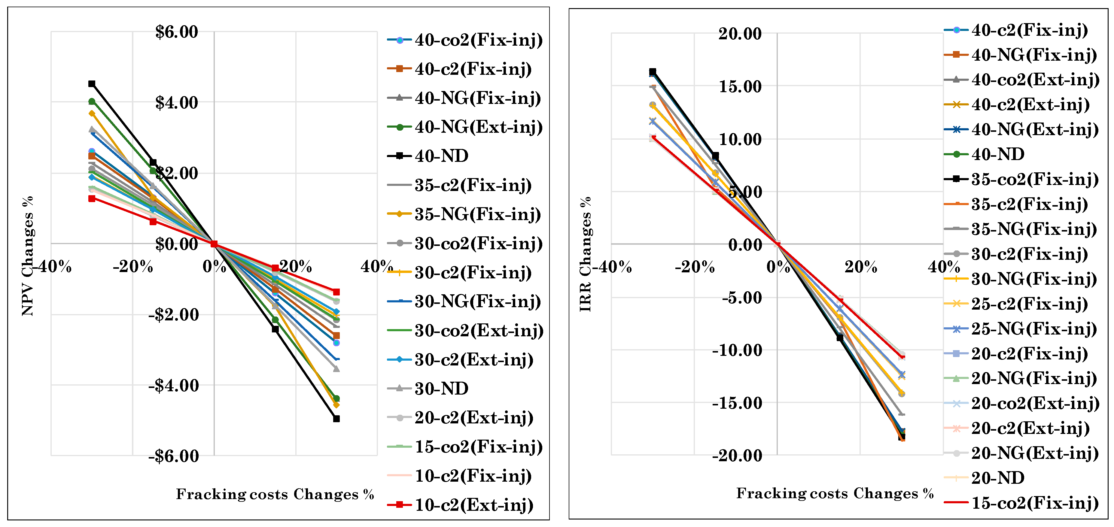
• Fracking cost has fewer effects on the profit compared with oil price. If the fracking cost decreases by 30% and 15%, NPV increases by 1.29% to 4.59% and 0.7% to 2.31% respectively. 30% and 15% increase in fracturing costs results in 9.96% and 1.36 decrease in NPV.
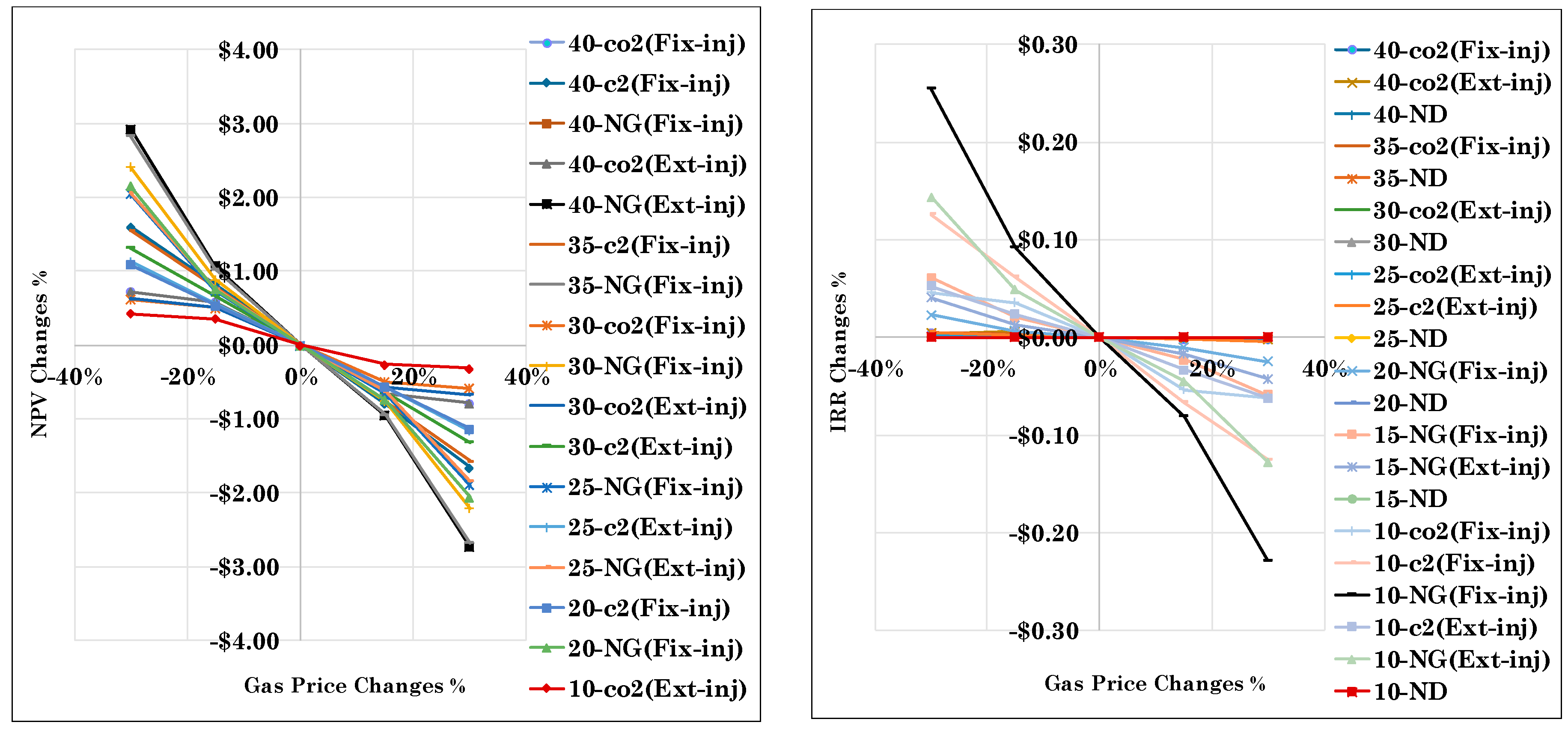
• Gas price is the factor with minimum effect on the economic responses. 30% and 15% reduction in gas prices lead to 0.43–2.93% and 0.38% to 1.05% increment in NPVs respectively. The scenario with the most benefit is FS = 40-NG (fixed and extended) and scenario with the least profit is FS = 10-CO₂ (extended). 30% and 15% increase in gas price yields to 0.31–2.73% and 0.26–0.91% incremental in NPV.
• Scenarios with minimum influences on the project’s economic in terms of NPV are fracking cost for n = 10-C₂ (extended), oil price for n = 30-C₂ (extended) and gas price for n = 10-CO₂ (extended).

References

1. U.S. Geological Survey 2013 Assessment of Undiscovered Resources in the Bakken and Three Forks Formations of the U.S. Williston Basin Province. Available online: https://pubs.er.usgs.gov/publication/70145284 (accessed on 9 April 2019).
2. U.S. Energy Information Administration (EIA). Available online: https://www.eia.gov/ (accessed on 9 April 2019).
3. Kolb, R.W. The Natural Gas Revolution: At the Pivot of the World’s Energy Future, 1st ed.; Pearson FT Press: Upper Saddle River, NJ, USA, 2013. [Google Scholar]
4. Drilling Productivity Report. Available online: https://www.eia.gov/petroleum/drilling/pdf/dpr-full.pdf (accessed on 9 April 2019).
5. Kulkarni, M.M. Immiscible and Miscible Gas-Oil Displacements in Porous Media. Master’s Thesis, Louisiana State University, Baton Rouge, LA, USA, 2003. [Google Scholar]
6. Moritis, G. EOR Survey. Oil Gas J. 2006, 104, 37–57. [Google Scholar]
7. IEA. CO2 Storge in Depleted oil Fields Report of the Greenhouse R&D Programme; IEA: Paris, France, 2009. [Google Scholar]
8. Bardon, C.; Corlay, P.; Longeron, D.; Miller, B. CO2 Huff ‘n’Puff Revives Shallow Light-Oil-Depleted Reservoirs. SPE Reserv. Eng. 1994, 9, 92–100. [Google Scholar] [CrossRef]
9. Mohammed, S.; Jennifer, L.; Singhal, A.K.; Sim, S.S. Screening criteria for CO2 huff‘n’puff operations. In Proceedings of the SPE/DOE Symposium on Improved Oil Recovery, Tulsa, OK, USA, 22–26 April 2006; Society of Petroleum Engineers: Houston, TX, USA, 2006. [Google Scholar]
10. Zhang, Y.P.; Sayegh, S.G.; Huang, S.; Dong, M. Laboratory Investigation of Enhanced Light-Oil Recovery by CO/Flue Gas Huff-n-Puff Process. J. Can. Petrol. Technol. 2004, 45. [Google Scholar] [CrossRef]
11. Koottungal, L. Worldwide EOR Survey. Oil Gas J. 2014, 112, 79–91. [Google Scholar]
12. Tunio, S.Q.; Tunio, A.H.; Ghirano, N.A.; El Adawy, Z.M. Comparison of different enhanced oil recovery techniques for better oil productivity. Int. J. Appl. Sci. Technol. 2011, 1, 143–153. [Google Scholar]
13. Yu, W.; Lashgari, H.; Sepehrnoori, K. Simulation study of CO2 huff-n-puff process in Bakken tight oil reservoirs. In Proceedings of the SPE Western North American and Rocky Mountain Joint Meeting, Denver, CO, USA, 16–18 April 2014. [Google Scholar]
14. Alharthy, N.; Teklu, T.; Kazemi, H.; Graves, R.; Hawthorne, S.; Braunberger, J.; Kurtoglu, B. Enhanced oil recovery in liquid-rich shale reservoirs: Laboratory to field. In Proceedings of the SPE Annual Technical Conference and Exhibition, Houston, TX, USA, 17–18 April 2015. [Google Scholar]
15. Hawthorne, S.B.; Gorecki, C.D.; Sorensen, J.A.; Steadman, E.N.; Harju, J.A.; Melzer, S. Hydrocarbon mobilization mechanisms from upper, middle, and lower Bakken reservoir rocks exposed to CO2. In Proceedings of the SPE Unconventional Resources Conference, Calgary, ON, Canada, 5–7 November 2013. [Google Scholar]
16. Todd, M.R.; Cobb, W.M.; McCarter, E.D. CO2 flood performance evaluation for the Cornell Unit, Wasson San Andres field. J. Petrol. Technol. 1982, 34, 2–271. [Google Scholar] [CrossRef]
17. Hsu, C.F.; Morell, J.I.; Falls, A.H. Field-scale CO2 flood simulations and their impact on the performance of the Wasson Denver unit. SPE Reserv. Eng. 1997, 12, 4–11. [Google Scholar] [CrossRef]
18. Asghari, K.; Dong, M.; Shire, J.; Coleridge, T.J.; Nagrampa, J.; Grassick, J. Development of a correlation between performance of CO2 flooding and the past performance of waterflooding in Weyburn oil field. SPE Prod. Oper. 2007, 22, 260–264. [Google Scholar] [CrossRef]
19. Wan, T. Evaluation of the EOR Potential in Shale Oil Reservoirs by Cyclic Gas Injection. Ph.D. Thesis, Texas Tech University, Lubbock, TX, USA, 2013. [Google Scholar]
20. Sheng, J.J.; Mody, F.; Griffith, P.J.; Barnes, W.N. Potential to increase condensate oil production by huff-n-puff gas injection in a shale condensate reservoir. J. Nat. Gas Sci. Eng. 2016, 28, 46–51. [Google Scholar] [CrossRef]
21. Li, L.; Sheng, J.J.; Xu, J. Gas Selection for huff-n-puff EOR in shale oil reservoirs based upon experimental and numerical study. In Proceedings of the SPE Unconventional Resources Conference, Calgary, AB Canada, 15–16 February 2017; Society of Petroleum Engineers: Houston, TX, USA, 2017. [Google Scholar]
22. Ali, S.; Farouq, M.; Thomas, S. A Realistic Look at Enhanced oil Recovery. Sci. Iran. 1994, 1, 3. [Google Scholar]
23. Hejazi, S.H.; Assef, Y.; Tavallali, M.; Popli, A. Cyclic CO2-EOR in the Bakken Formation: Variable cycle sizes and coupled reservoir response effects. Fuel 2017, 210, 758–767. [Google Scholar] [CrossRef]
24. Zhou, S.; Zhuang, X.; Rabczuk, T. A phase-field modeling approach of fracture propagation in poroelastic media. Eng. Geol. 2018, 240, 189–203. [Google Scholar] [CrossRef]
25. Cockin, A.P. Prudhoe Bay Miscible Gas Distribution. In Proceedings of the SPE Western Regional Meeting, Anchorage, AK, USA, 26–28 May 1993; Society of Petroleum Engineers: Houston, TX, USA, 1993. [Google Scholar]
26. DeRuiter, R.A.; Nash, L.J.; Singletary, M.S. Solubility and displacement behavior of a viscous crude with CO2 and hydrocarbon gases. SPE Reserv. Eng. 1994, 9, 101–106. [Google Scholar] [CrossRef]
27. Sharma, G.D. Development of Effective Gas Solvents Including Carbon Dioxide for the Improved Recovery of West Sak Oil. No. DOE/FE/61114-2; Alaska Univ., Petroleum Development Lab.: Fairbanks, AK, USA, 1990. [Google Scholar]
28. McGuire, P.L.; Okuno, R.; Gould, T.L.; Lake, L. Ethane-based EOR: An innovative and profitable EOR opportunity for a low price environment. In Proceedings of the SPE Improved Oil Recovery Conference, Tulsa, OK, USA, 11–13 April 2016; Society of Petroleum Engineers: Houston, TX, USA, 2016. [Google Scholar]
29. Natural Gas Futures Contract 1. Available online: https://www.eia.gov/dnav/ng/hist/rngc1A.htm (accessed on 4 November 2018).
30. Natural Gas Prices Are a Function of Market Supply and Demand. Available online: https://www.eia.gov/energyexplained/index.cfm?page=natural_gas_factors_affecting_prices (accessed on 19 December 2018).
31. Assef, Y.; Almao, P.P.; Pourafshary, P. Miscibility Effects on Performance of Cyclic CO2 Injection in Hysteretic Tight Oil Reservoirs. In Proceedings of the Abu Dhabi International Petroleum Exhibition & Conference, Abu Dhabi, UAE, 12–15 November 2018; Society of Petroleum Engineers: Houston, TX, USA, 2018. [Google Scholar]
32. Assef, Y.; Kantzas, A.; Almao, P.P. Numerical modelling of cyclic CO2 injection in unconventional tight oil resources; trivial effects of heterogeneity and hysteresis in Bakken formation. Fuel 2019, 236, 1512–1528. [Google Scholar] [CrossRef]
33. Tabrizy, V.A. Investigated Miscible CO2 Flooding for Enhancing Oil Recovery in Wettability Altered Chalk and Sandstone Rocks. Ph.D. Thesis, University of Stavanger, Stavanger, Norway, 2012. [Google Scholar]
34. Hawthorne, S.B.; Miller, D.J.; Jin, L.; Gorecki, C.D. Rapid and simple capillary-rise/vanishing interfacial tension method to determine crude oil minimum miscibility pressure: Pure and mixed CO2, methane, and ethane. Energy Fuels 2016, 30, 6365–6372. [Google Scholar] [CrossRef]
35. Hawthorne, S.B.; Miller, D.J.; Sorensen, J.A.; Gorecki, C.D.; Steadman, E.N.; Harju, J.A. Effects of reservoir temperature and percent levels of methane and ethane on CO2/Oil MMP values as determined using vanishing interfacial tension/capillary rise. Energy Procedia 2017, 114, 5287–5298. [Google Scholar] [CrossRef]
36. Trends in U.S. Oil and Natural Gas Upstream Costs, Independent Statistics & Analysis. U.S. Energy Information Administration. Available online: www.eia.gov (accessed on 23 March 2016).
37. 2015 Carbon Dioxide Price Forecast. Available online: http://www.synapse-energy.com/sites/default/files/2015%20Carbon%20Dioxide%20Price%20Report.pdf (accessed on 3 March 2015).
38. Hydrocarbon Gas Liquid Prices Are Related to Oil and Natural Gas Prices and Are Related to Supply and Demand. Available online: https://www.eia.gov/energyexplained/index.cfm?page=hgls_prices (accessed on 19 December 2018).
39. Short-Term Energy Outlook. Available online: https://www.eia.gov/outlooks/steo/report/natgas.php (accessed on 9 April 2019).
40. Canada’s Energy Future 2016: Energy Supply and Demand Projections to 2040. Available online: https://www.neb-one.gc.ca/nrg/ntgrtd/ftr/2016/index-eng.html (accessed on 9 April 2019).
41. What is the Formula for Calculating Net Present Value (NPV)? Available online: https://www.investopedia.com/ask/answers/032615/what-formula-calculating-net-present-value-npv.asp (accessed on 9 April 2019).
Figure 1. Schematic of two hydraulic fractures (HF) and SRV area with local grid refinement. SRV length is 450 ft. SRV width is variable; depending on fracture spacing.
Energies 12 01370 g001
Figure 2. Primary (natural depletion) recovery factor at different number of fracture stages.
Energies 12 01370 g002
Figure 3. Dashed lines: average reservoir pressure; solid lines: oil recovery factor during CGI in both fixed and growing cycle sizes for n = 10.
Energies 12 01370 g003
Figure 4. Dashed lines: average reservoir pressure; solid lines: oil recovery factor during CGI in both fixed and growing cycle sizes for n = 35.
Energies 12 01370 g004
Figure 5. Composition of oil before and after natural depletion (ND) and CGI by CO2, C2H6 and NG.
Energies 12 01370 g005
Figure 6. Composition of oil before and after natural depletion (ND) and CGI by CO2, C2H6 and NG.
Energies 12 01370 g006
Figure 7. IFT during natural depletion (ND) and CGI by CO2, C2H6 and NG, Oil API = 38°.
Energies 12 01370 g007
Figure 8. IFT during natural depletion (ND) and CGI by CO2, C2H6 and NG, Oil API = 31°.
Energies 12 01370 g008
Figure 9. Average reservoir pressure after one year of natural depletion for different fracture stages (FS).
Energies 12 01370 g009
Figure 10. C2H6 Injection (Fixed Cycle Size) 38 API Oil.
Energies 12 01370 g010
Figure 11. C2H6 Injection (Extended Cycle Size) 38 API Oil.
Energies 12 01370 g011
Figure 12. CO2 Injection (Fixed Cycle Size) 38 API Oil.
Energies 12 01370 g012
Figure 13. CO2 Injection (Extended Cycle Size) 38 API Oil.
Energies 12 01370 g013
Figure 14. NG Injection (Fixed Cycle Size) 38 API Oil.
Energies 12 01370 g014
Figure 15. NG Injection (Extended Cycle Size) 38 API Oil.
Energies 12 01370 g015
Figure 16. C2H6 Injection (Fixed Cycle Size) 31 API Oil.
Energies 12 01370 g016
Figure 17. C2H6 Injection (Extended Cycle Size) 31 API Oil.
Energies 12 01370 g017
Figure 18. CO2 Injection (Fixed Cycle Size) 31 API Oil.
Energies 12 01370 g018
Figure 19. CO2 Injection (Extended Cycle Size) 31 API Oil.
Energies 12 01370 g019
Figure 20. NG Injection (Fixed Cycle Size) 31 API Oil.
Energies 12 01370 g020
Figure 21. NG Injection (Extended Cycle Size) 31 API Oil.
Energies 12 01370 g021
Figure 22. NPV of the scenarios for fixed and extended cycles of cyclic CO2, C2 and NG injection as well as natural depletion, FS = 30, Oil API = 38.
Energies 12 01370 g022
Figure 23. Cumulative NPV of the scenarios for fixed and extended cycles of cyclic CO2, C2 and NG injection as well as natural depletion, FS = 30, Oil API = 38.
Energies 12 01370 g023
Figure 24. NPV of the scenarios for fixed and extended cycles of cyclic CO2, C2 and NG injection as well as natural depletion, FS = 10, Oil API = 38.
Energies 12 01370 g024
Figure 25. Cumulative NPV of the scenarios for fixed and extended cycles of cyclic CO2, C2 and NG injection as well as natural depletion, FS = 10, Oil API = 38.
Energies 12 01370 g025
Figure 26. NPV of the scenarios for fixed and extended cycles of cyclic CO2, C2 and NG injection as well as natural depletion, FS = 30, Oil API = 31.
Energies 12 01370 g026
Figure 27. Cumulative NPV of the scenarios for fixed and extended cycles of cyclic CO2, C2 and NG injection as well as natural depletion, FS = 30, Oil API = 31.
Energies 12 01370 g027
Figure 28. NPV of the scenarios for fixed and extended cycles of cyclic CO2, C2 and NG injection as well as natural depletion, FS = 10, Oil API = 31.
Energies 12 01370 g028
Figure 29. Cumulative NPV of the scenarios for fixed and extended cycles of cyclic CO2, C2 and NG injection as well as natural depletion, FS = 10, Oil API = 31.
Energies 12 01370 g029
Figure 30. Changes in NPV and IRR coming from variation in fracking costs.
Energies 12 01370 g030
Figure 31. Changes in NPV and IRR coming from variation in Oil Price.
Energies 12 01370 g031
Figure 32. Changes in NPV and IRR coming from variation in Gas Price.
Energies 12 01370 g032
Figure 33. Changes in NPV and IRR coming from variation in fracking costs.
Energies 12 01370 g033
Figure 34. Changes in NPV and IRR coming from variation in Oil Price.
Energies 12 01370 g034
Figure 35. Changes in NPV and IRR coming from variation in Gas Price.
Energies 12 01370 g035