Article

Finite-Volume High-Fidelity Simulation Combined with Finite-Element-Based Reduced-Order Modeling of Incompressible Flow Problems

1
Department of Mathematical Sciences, Norwegian University of Science and Technology, NO-7491 Trondheim, Norway
2
CSE Group, Mathematics and Cybernetics, Sintef Digital, NO-7034 Trondheim, Norway
*
Author to whom correspondence should be addressed.
Energies 2019, 12(7), 1271; https://doi.org/10.3390/en12071271
Submission received: 13 February 2019 / Revised: 19 March 2019 / Accepted: 1 April 2019 / Published: 2 April 2019
(This article belongs to the Special Issue Recent Advances in Aerodynamics of Wind Turbines)

Abstract

:
We present a nonintrusive approach for combining high-fidelity simulations using Finite-Volume (FV) methods with Proper Orthogonal Decomposition (POD) and Galerkin Reduced-Order Modeling (ROM) methodology. By nonintrusive we here imply an approach that does not need specific knowledge about the high-fidelity Computational Fluid Dynamics (CFD) solver other than the velocity and pressure results given on an element mesh representing the related discrete interpolation spaces. The key step in the presented approach is the projection of the FV results onto suitable finite-element (FE) spaces and then use of classical POD Galerkin ROM framework. We do a numerical investigation of aerodynamic flow around an airfoil cross-section (NACA64) at low Reynolds number and compare the ROM results obtained with high-fidelity FV-generated snapshots against similar high-fidelity results obtained with FE using Taylor–Hood velocity and pressure spaces. Our results show that we achieve relative errors in the range of 1–10% in both H 1 -seminorm of the computed velocities and in the L 2 -norm of the computed pressure with reasonably few ROM modes. Similar accuracy was obtained for lift and drag.

1. Introduction

High-fidelity numerical simulations based on finite-volume (FV) method [1], finite-element (FE) method [2] and finite-difference (FD) method [3] are generally used to study phenomena governed by partial differential equations [4]. In the context of incompressible fluid flow, these equations are called the Navier–Stokes equations and the branch of computational techniques that deals with it called the Computational Fluid Dynamics (CFD) [5]. The solution of these equations for complicated flows around complex geometries such as a turbine blade [6] requires high degrees of freedom and hence are computationally very demanding even on the most advanced computing facilities [7,8]. The industry, on the other hand, has a need for accurate yet computationally light modeling tools for design optimization and real-time predictions. To this end, researchers have been developing reduced-order models. One such development in the field is towards the use of self-excited oscillator models for prediction of the aerodynamic forces (drag and lift) on the bluff bodies [9,10]. Others have exploited reduced basis methods for higher-dimensional systems by extracting the most useful information from the flow field [11,12,13]. In a reduced basis method, high-fidelity numerical simulation results for a set of input parameters are projected onto a significantly lower-dimensional space to construct reduced basis which is then used to build up a reduced-order model [14,15,16]. Such models exhibit efficiency, robustness, reliability, and accuracy.
Usually, the aerodynamic flow-related problems in wind engineering depend heavily on some critical parameters such as angle of attack, wind velocity, airfoil shape, etc. [17]. For faster-repeated sampling, it could be a legitimate alternative to approximate the behavior based on a linear combination of precomputed solutions on a reduced basis for different choices of input parameter space (physical or geometrical) [18]. This required transformation of the non-affine problems in an affine way which—to the best of the knowledge of the authors—have not been addressed before for wind turbines, where the angle of attack undergoes periodic variations over a complete cycle. Concerning order reduction procedures, known methods to develop the basis in the literature are Greedy Method (GM), Centroidal Voronoi Tessellations (CVT) Taylor, Lagrange, Hermite, and Proper Orthogonal Decomposition (POD) [19]. The techniques provide a subspace which optimally represents a dynamical system with fewer degrees of freedom [20,21]. The dominant modes after the decomposition capture the highly energetic coherent structures in a flow field [22,23,24].
To perform POD, input data sets are required and taken from experiments or numerical studies. The reduced basis obtained from POD is ordered by descending energy content and termed as basis functions or modes [25]. The first use of POD in engineering applications was formally introduced in the study by authors [26,27], who employed the technique to study the formation of coherent structures in a flow field. Later, authors of [20,28] used it to solve problems related to boundary layer turbulence. The author of [29] used FE technique to generate the snapshots and analyzed the turbulent structures using POD around a circular cylinder. The author of [30] extended that technique to develop a Galerkin free POD formulation of incompressible flows using snapshots from a DNS solver. The authors of [31] developed a minimum residual projection to build coupled velocity-pressure POD-ROM for incompressible Navier–Stokes equations using the high-fidelity data from the FE approach. The new model enabled to increase the velocity and pressure fields accuracy. The authors of [11] employed POD to develop a Galerkin ROM for the construction of both pressure and velocity spaces. They adopted an enrichment procedure of the velocity space by supremizer solutions to enhance the stability and monitored the fulfillment of an inf-sup Ladyzhenskaya–Babuska–Brezzi (LBB) stability condition at the reduced-order level. Whereas studies related to the affine representation of velocity and pressure fields are important and based on the reduced basis and a transformation between physical and reference geometries. The authors of [32] employed the strategy and developed a ROM for the Stokes problem using a domain decomposition technique. The author of [24] has shown the integration of FVM and POD, whereas authors of [16] demonstrated the applicability of such an approach on a two-dimensional cylinder.
In this paper, the concept of mixing of methods for the development of novel FE-based ROM is demonstrated. We devised mixed method term for the reduced FE solution obtained from the snapshots generated by FV method. Whereas, uniform method is called for the reduced FE solution based on the snapshots created by FE method. The methods are implemented, and their applicability is manifested on a parametrized two-dimensional NACA64 airfoil. For a combination of input physical (velocity) and geometrical (incidence angle) parameters, high-fidelity simulations of FE and FV are conducted using an in-house code and OpenFOAM (4.0) [33] respectively. First, an optimal reduced basis is constructed on the reference domain with the application of POD on the snapshots generated using FE and FV methods. Using the reduced space, a reduced-order model based on FE method is formed in the Nutils [34] framework. The ROM solutions are compared with the corresponding FE, and FV high-fidelity discretization and the differences are illustrated in the energy spectrum, error magnitudes, computational time for the methods and the shape of the modes. Supremizer solutions are added to the velocity space such that non-spurious pressure modes can be developed resulting in a stable solution. The whole procedure is demonstrated with a novel procedure, that transforms wind turbine-related problems from a classical non-affine context to an affine framework thereby motivating the use of precomputed solutions as a linear combination of reduced basis functions.
In this paper, Section 2 describes the systems of governing equations, the discretization technique for the map and the affine transformation. The formulation of reduced-order modeling (ROM) is then presented in Section 3. The section also describes the implementation of our solver and boundary conditions. In Section 4, the results are compared for the two developed models in terms of flow dynamics, spectrum of velocity/pressure, L 2 error and the computational efficiencies evaluated in a test case of the NACA64 airfoil. The last section describes the conclusions of the work followed by future recommendations.

2. Theory

This section describes the mathematical formulation of the reduced assembly based on the governing equations, the POD, and the affine representation of the equations.

2.1. Governing Equations

The steady Navier–Stokes equations can model the flow in a low Reynolds number regime, where the equations are non-linear due to the presence of the convection term [35]. The equations are considered for the cases when ν is constant. The flow remains incompressible below the Mach number of 0.3. The mathematical description of the Navier-Stoke equations is given as
ν Δ u + ( u · ) u + p = f in Ω , · u = 0 in Ω , u = g on Γ D , p n + ν ( u ) n = h on Γ N .
The equation represents distributive force f , Dirichlet data g and Neumann fluxes h where ν is the kinematic viscosity, u = ( u 1 , u 2 ) is the velocity field, p, is the pressure and n shows the normal unit vector to Γ N . The domain of interest is represented by Ω R d , with mixed boundary conditions. Figure 1 represents the boundaries of the domain, where a solid line at the inlet illustrates Dirichlet ( Γ D ) and the dotted line represents the Neumann ( Γ N ) conditions at the boundary. The mathematical description of boundary is introduced as
Ω = Γ D Γ N , Γ D Γ N = , Γ D .

2.1.1. FE Discretization

The discretization of the Navier–Stokes equations is developed by determining the weak variational formulation of our problem [36,37]. To manage the inhomogeneous Dirichlet boundary conditions, a lifting function is constructed corresponding to the Dirichlet boundary condition such that = g on Γ D , writing u = u 0 + where u 0 satisfies homogeneous Dirichlet conditions u 0 = 0 on Γ D . The governing equations are multiplied with the test functions ( w , q) and perform integration by parts to obtain the solution onto the physical domain. Hence, the weak form is described as
d ¯ ( u 0 , w ) + c ( u 0 , u 0 , w ) + b ( p , w ) = f ¯ 1 ( w ) ,
b ( q , u 0 ) = b ( q , ) .
the bi- and trilinear forms are defined as
d ¯ ( u 0 , w ) = d ( u 0 , w ) + c ( u 0 , , w ) + c ( , u 0 , w ) ,
f ¯ 1 ( w ) = Γ N h · w + Ω f · w d ( , w ) c ( , , w ) ,
d ( v , w ) = ν Ω v : w ,
b ( p , w ) = Ω p · w ,
c ( z , v , w ) = Ω ( z · ) v · w .
For Galerkin discretization, we then choose finite dimensional subspaces U h U , P h P , U 0 h = v U h | v = 0 on Γ D and wish to find ( u 0 , p ) U 0 h × P n such that (1) and (2) hold for all ( w , q ) U h × P h .
Specifically, let Ω = i K e be a decomposition of the computation domain into quadrilateral pairwise disjoint elements K e , and for each element, define a mapping
π e : K e > [ 0 , 1 ] 2
Given a selection of shape functions defined on the reference element [ 0 , 1 ] 2 , we can then define the corresponding shape functions on K e by pullbacks through π e . With this in mind, let us define on [ 0 , 1 ] 2 the bilinears and biquadratics,
Q 1 , 1 = span 1 , ξ , η , ξ η Q 2 , 2 = span 1 , ξ , η , ξ η , ξ 2 , η 2 , ξ 2 η , ξ η 2 , ξ 2 η 2
and define our finite dimensional subspaces as globally C 0 -continuous biquadratics and bilinears [38], respectively. These are also known as Taylor–Hood [39] type elements.
U h = v H 1 ( Ω ) 2 C 0 ( Ω ) 2 | π e * v Q 2 , 2 2 e P h = p L 2 ( Ω ) C 0 ( Ω ) | π e * p Q 1 , 1 e .

2.1.2. FV Discretization

The Navier–Stokes equations in space are discretized using the FV approximation technique. The PDEs are discretized over the control volume using the integral form approach. To avoid additional errors due to the differences between the domain subdivisions into finite cells/elements, the same number of non-overlapping cells are used in both methods. The discretized equations for momentum and continuity are represented for each term using the Gauss theorem which converts the volume integrals into surface integrals [40]. The integral form of the momentum equation over each control volume is given by
V ( u · ) u d V ν V Δ u d V + V p d V = 0
Here, the discretization of each term in the Navier–Stokes is discussed explicitly. The convective term, using the linear variation of u and applying the generalized form of Gauss theorem is discretized
V ( u · ) u d V = V · ( u u ) d V = S d S f · ( u u ) f S f · u f u f = f F u f
the u f represents the velocity at the center of the face of the control volume. where S f is the surface area of the face and F is the face flux. The F represents the mass flux over the surface of each face constituting the control volume. It is formed from the product of S f · u f .
The Laplacian, continuity, and pressure terms are discretized as follows
V · ( ν u ) d V = S d S f · ( ν u ) f ν S f · ( u ) f = ν f F
V · u d V = S d S · ( u ) = f S f · u f = f F
V p d V = S d S · ( p ) = f S f · p
p represents the values at the center of each control face of the control volume. The integrals appearing in the equations above are linearized employing the first/second-order upwind, blended difference, and the central differencing schemes available in OpenFOAM (4.0) [33]. The continuity equation is solved taking the divergence of momentum and solving as pressure Poisson equation. For further explanation, the reader is referred to [33]. The schemes used for the solution of numerical examples are described in Section 4.1.

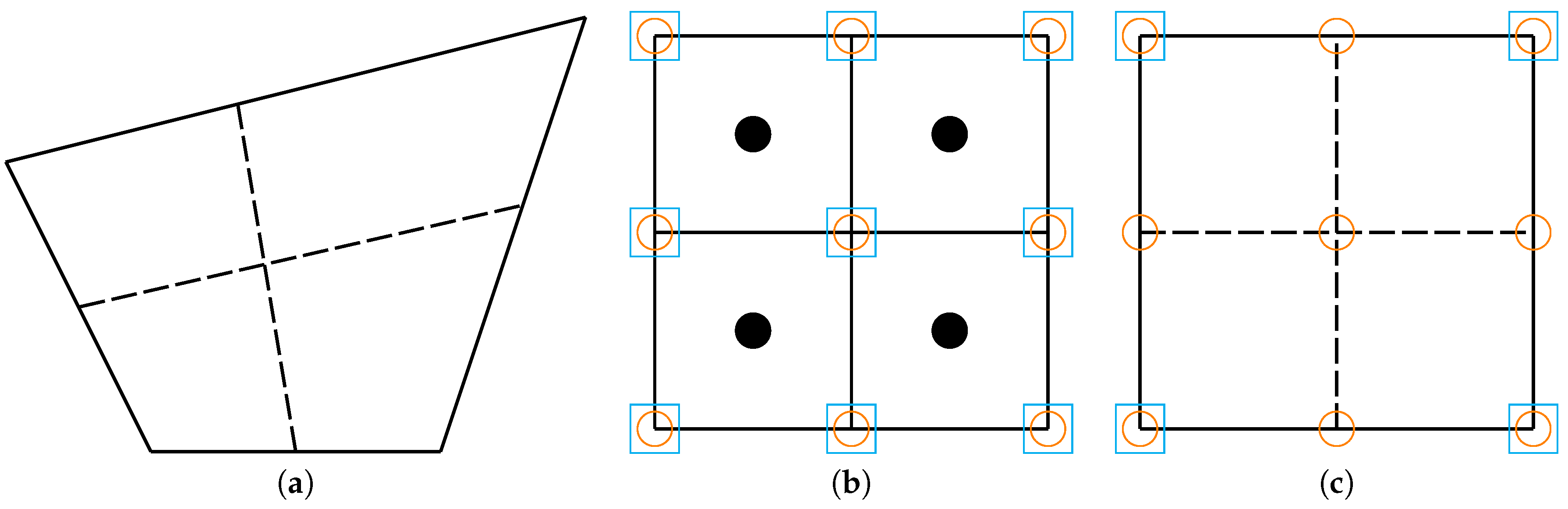
2.2. Projection of FV Results to FE Space

Earlier work on combining the FV high-fidelity solvers with POD Galerkin ROM is presented in [16,24]. They have adopted a consistent approach and included the contribution of the face flux field (face area vector multiplied by the face flux) in addition to the velocity and pressure fields into the POD Galerkin ROM. This is done to ensure that the method employed to construct the ROM remain consistent with the Full-order Model (FOM). However, the drawback with this is that it introduces an extra field variable and that it requires access to the high-fidelity face flux field, which is not always easily accessible.
Herein, we explore a nonintrusive approach, i.e., no specific knowledge is needed about the high-fidelity CFD solver other than the velocity and pressure snapshots given on an element mesh representing the related discrete interpolation spaces. The key step in our approach is that the FV high-fidelity velocity and pressure fields are projected onto suitable FE spaces and then the classical POD Galerkin ROM algorithm is applied. Unfortunately, the projection from FV-spaces to FE spaces introduces an inconsistency between the FV-FOM and the resulting ROM, i.e., the projected high-fidelity FV velocities and pressures do not fulfill Equations (1) and (2). The significance of this inconsistency error relative to the error introduced by ROM is an important issue in our numerical investigation presented below.
We have used OpenFOAM in this study to produce the high-fidelity FV results and the computed velocities and pressures are transferred to the Taylor–Hood FE space in a two-stage process:
  • Cell centers to cell nodes interpolation:
    In the first stage, the velocity and pressure fields that are calculated by OpenFOAM at the center of the control volumes are interpolated onto the control volume vertices using Inverse Distance Weighting (IDW) interpolation before they are stored at VTK-files. Thus, the stored velocity and pressure results on the VTK-files are implicitly assumed to be interpolated as bilinear fields.
  • Projection to taylor hood FE space:
    In the second stage, the velocity and pressure results stored on the VTK-files are projected onto the Taylor–Hood FE space. Herein, we have used L 2 -projection for both velocities and pressure.
To minimize the inconsistency error, we generated first the FE-mesh with characteristic element size 2 h and then uniformly refined every element into four new elements with characteristic element size h. As illustrated in Figure 2a this was done in such a way that the geometry of the domains Ω h and Ω 2 h is exactly the same for the two different meshes.
The Taylor–Hood FE space is characterized by biquadratic interpolation of velocities and bilinear interpolation of the pressure, whereas the OpenFOAM results stored on the VTK-files are assumed interpolated bi-linearly for both variables. We have here chosen to project the FV results computed on a mesh with characteristic size h onto an FE-mesh of characteristic size 2 h as this gives the same number of degrees of freedoms (DOFs) for the FV and FE velocity fields. Furthermore, the original FV results are piecewise (cell-centered) constant, and therefore considered to be less accurate than Taylor–Hood FE of the same mesh size.

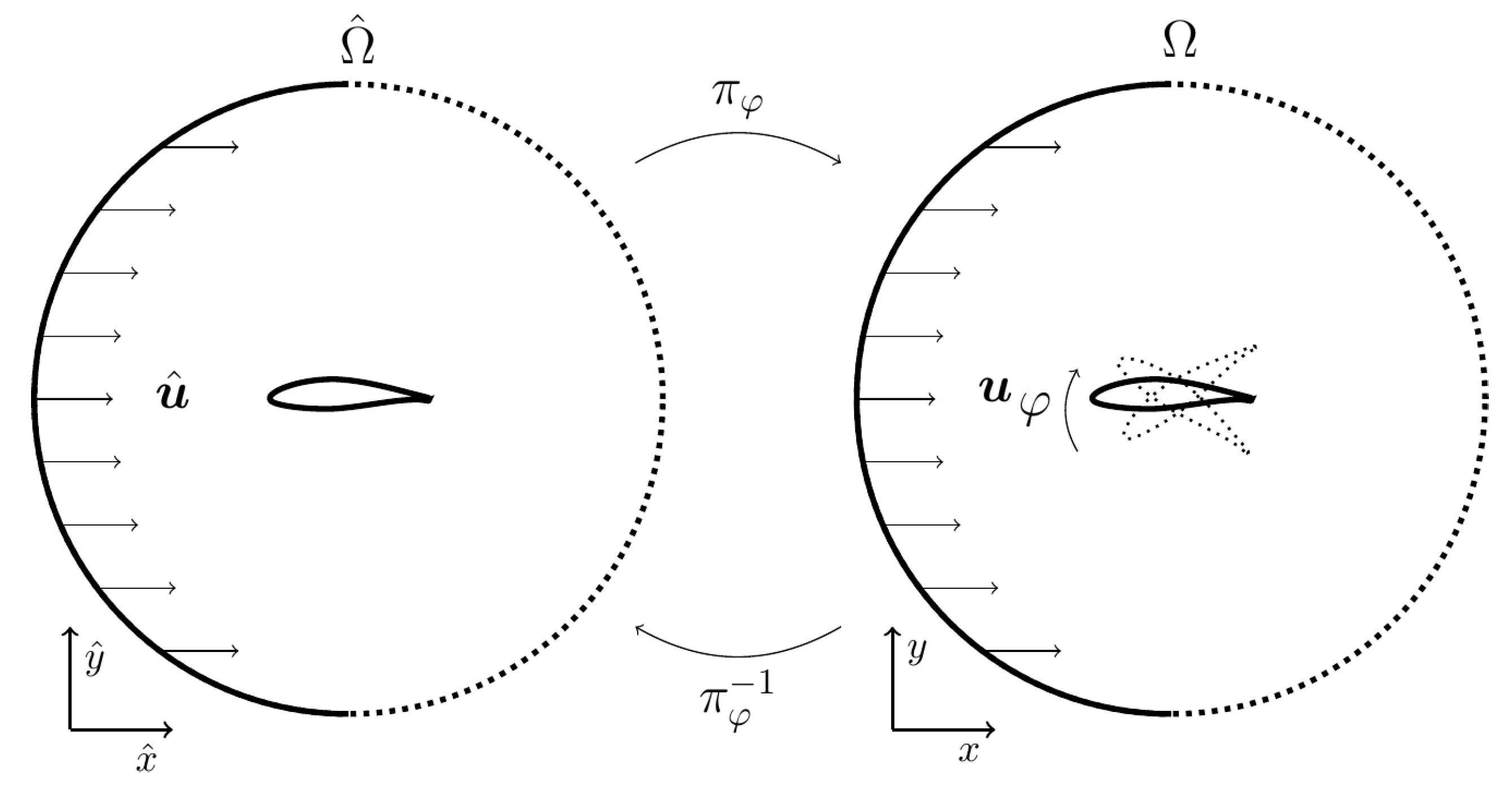
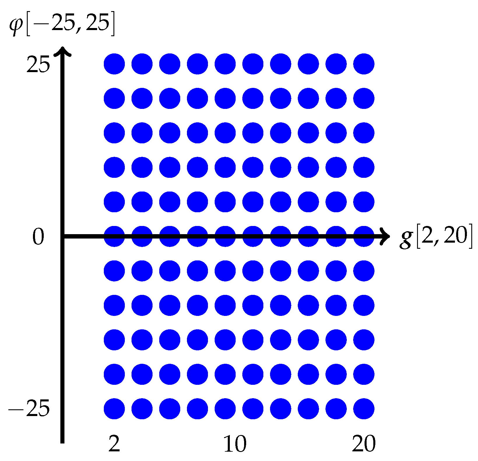
2.3. Parametric Dependency

We consider here the case where the problem defined by (1) and (2) is depends on several parameters. Denote by P the parameter space and by μ any given element of P . For flow problems we typically have the following classes of parameters: physical parameters, boundary condition parameters and geometric parameters. We shall denote the linear and bilinear forms dependence on the parameters μ with notation such as d ( u , w ; μ ) , and similarly for other forms.
Physical parameters are very often material parameters describing the continuum at hand e.g., the viscosity ν of an incompressible fluid. Boundary condition parameters are related to the Dirichlet and Neumann conditions, e.g., g and h in the governing equations of the Navier–Stokes equation. In particular, non-homogeneous Dirichlet parameters g (that introduce the lifting function l) needs to be handled properly [41].
Geometric parameters imply that the computational domain Ω = Ω ( μ ) varies. Let Ω ^ be a reference domain which herein is described by the physical domain of Ω ( μ 2 = φ = 0 ) (i.e., angle of attack equal to zero) and a corresponding FE and FV discretization of Ω ^ . A one-to-one mapping is then introduced to map the physical domain to the reference geometry and is defined by
π μ : Ω ^ ( μ ) Ω .
Suitable functions are created in the physical domain Ω ( φ ) by applying the pullback on the transformation which maps the solution from the reference geometry onto the physical geometry and is given by (see [41] for more details)
v = π μ * v ^ , p = π μ * p ^ .
The geometry variation affects the linear and bilinear forms. Hence for the convective form c, the mapping takes the form
c ( π φ * u ^ , π φ * v ^ , π φ * w ^ ; φ ) = Ω ^ ( u ^ · J ) v ^ · w ^ i = 0 2 n φ i Ω ^ ( u ^ · B i ( ) ) v ^ · w ^ .
and for the diffusive part d it reads
d ( π φ * u ^ , π φ * w ^ ; φ ) = ν Ω ^ ( J ) u ^ : ( J ) w ^ = ν Ω ^ u ^ : ( J 1 J ) w ^ ,
and finally, the incompressibility constraints b becomes
b ( π φ * p ^ , π φ * w ^ ; φ ) = Ω ^ p ^ ( J ) · w ^ = Ω ^ p ^ J : w ^ ,
To find the detail derivation of the above ROM equations and the explanation of expressions B i ( ) the reader is referred to the article by Fonn et al. [41]

2.4. ROM Using POD

The notion of ROM is introduced to obtain an accurate solution of the Navier–Stokes equations over a discrete solution space whose dimensions far exceeds the natural dimensions of the model itself [42]. In other words, the practical dimensions of the space
( u ^ 0 ( μ ) , p ( μ ) ) | μ P
is considerably more manageable than the dimension of any discretization necessary to achieve good accuracy with conventional FE/FV methods. We will solve the steady Navier–Stokes problem and proceed by sampling and generate the ensemble of solutions which corresponds to different snapshots to produce an approximation of the space of Equation (14). The POD is employed to reduce the dimension of the space such that the solution can be described by an optimal combination of the most energy rich modes [21,42].
First the ensemble is developed by performing the high-fidelity simulations at each state chosen by a combination of input parameters with FE and FV methods ( μ i = ( φ i , g i ))
Φ = ϕ i = ( u ^ 0 i ( φ i , g i ) , ( p ^ i ( φ i , g i ) i = 1 N
A correlation matrix is then constructed from the ensemble for velocity and pressure respectively,
C i j = a ( ϕ i , ϕ j )
Given eigenpairs ( λ i , v i ) of C , one may then pick an M such that
i = 1 M λ i 1 ϵ 2 i = 1 N λ i
where ϵ > 0 is a suitable error tolerance. It is hoped that M N , as M will be the dimension of the reduced space (it can be interpreted as the practical dimension of the space given by Equation (14) Error ϵ , as measured in the norm | | · | | a = ( a ( · , · ) ) . The reduced basis functions are then given by
ψ j = 1 λ j i = 1 N v i j ϕ i , 1 j M
It can be noted that the ψ j are orthonormal in the a ( · , · ) inner product [43]. In practice, this construction is performed separately on the velocity and pressure fields. Thus, first we choose a velocity correlation function
a u ( ( u 0 ^ , p ^ ) , ( v 0 ^ , q ^ ) ) = ( u 0 ^ , v 0 ^ ) L 2 ( Ω )
Secondly, we choose the pressure correlation function
a p ( ( u 0 ^ , p ^ ) , ( v 0 ^ , q ^ ) ) = ( p 0 ^ , q 0 ^ ) L 2 ( Ω )
The velocity and pressure basis are constructed as
u ^ j R = 1 λ j i = 1 N v i ( u ) , j u ^ 0 i , p ^ j R = 1 λ j i = 1 N v i ( p ) , j p ^ i , 1 j M

2.5. Mixed and Uniform Methods

Classical reduced basis methods generally use the same high-fidelity method both for constructing the ensemble and creating the reduced basis method itself. In other words, given that the ensemble solutions u ( μ i ) satisfy the equation
A ( μ i ) u ( μ i ) = b ( μ i ) ,
where A , b denote a parameter-dependent system matrix and right-hand side, respectively, the reduced system is given as
A R ( μ ) = V A ( μ ) V , b R ( μ ) = V b ( μ ) ,
the “tall” matrix V is generated from the relation between high-fidelity basis and the reduced-order basis as given in Equation (16)
( V T ) i j = v i j λ j
In the following, the above method will be denoted as uniform, to distinguish it from the mixed method. By the latter it is meant that a model is obtained by generating ensemble solutions with a given high-fidelity method ( 1 ) ,
A ( 1 ) ( μ i ) u ( μ i ) = b ( 1 ) ( μ i ) ,
and then using a different high-fidelity method ( 2 ) as a basis for the reduction, i.e.
A R ( μ ) = V A ( 2 ) ( μ ) V , b R ( μ ) = V b ( 2 ) ( μ ) .
This is motivated by the idea of enable nonintrusive ROM. So long as the two high-fidelity methods purport to solve the same physical model (and that this physical model accurately reflects reality), one may reasonably hope that mixing methods in this way will be sufficiently accurate.
In the following, the two high-fidelity methods used in the present study are the FE and FV methods described in Section 2.1.1 and Section 2.1.2 respectively. By the “Uniform” method, it is meant that the reduced model is based fully on the FE method, and by the “Mixed” method, it is meant that the snapshots (and therefore the basis) were generated with the FV method, but the method underlying the reduction was the FE method. As such, the difference between the two reduced models is entirely in their bases.

3. Development of the Solver

ROM Solver

The reduce space after the POD stage is obtained. The solution for the reduced-order model requires solving several systems of the form
A v v B v p B p v v p = b v b p
The matrix B v p is observed to be numerically rank-deficient, i.e., it has a nontrivial kernel, therefore leading to unstable pressure solutions. To remedy this, the velocity space is artificially enriched with supremizers basis functions whose purpose is not to achieve greater approximative power but rather to keep the system well-conditioned [11]. Therefore, for each pressure snapshot p ^ i , represented by the high-fidelity coefficient vector p , at a parameter μ i , to solve the system
M V ( μ i ) v = B ( μ i ) p
for the velocity coefficient vector v , which then yields the supremizer function at that particular parameter-value. Here, M V is the H 1 -norm mass matrix, and B is the matrix associated with the b ( · , · ; μ ) bilinear form.
The supremizers are then reduced using the POD as well, just like the regular velocity solutions, into a separate and independent reduced space, yielding the system
A v v A v s B v p A s v A s s B s p B p v B p s v s p = b v b s b p
In practice, the sizes of each basis are kept equal, so with M degrees of freedom each for velocity, supremizers and pressure, one obtains a 3 M -sized system [11].

4. Results and Discussion

The aim of the numerical investigation is to see how well the mixed method compares with the uniform method. In particular, we want to study the significance of the inconsistency error compared to the error introduced by choosing a reduced-order basis. Our aim regarding accuracy is to achieve a difference between the high-fidelity simulation and the reduced-order simulation in the range of 1–10% relative error in suitable norms for the quantity of interest.
In the following, we first describe in detail the high-fidelity simulation setup and the choice of parametric values for the snapshot creation. To introduce the study of the obtained ROM results we display the most energy-rich modes and corresponding spectrum of the reduced-order basis. Then we focus on the relative error convergence plots of H 1 -seminorm of the computed ROM-velocities and the L 2 -norm of the computed ROM-pressures. Similarly, we display the relative error convergence plot of the computed ROM lift and drag. We then report the parametric dependence of the difference in the FV and FE high-fidelity solutions. In the end, we report the observed speedup.

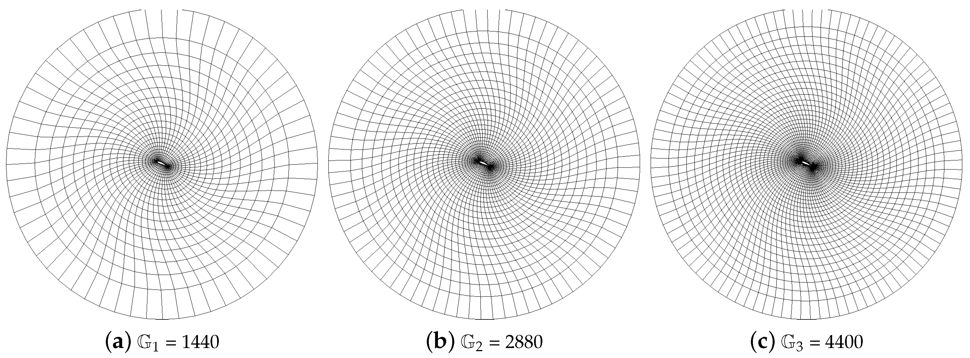
4.1. High-Fidelity Simulation Setup

The developed ROM is benchmarked on a two-dimensional NACA64, which is the airfoil located at the outer most section of NREL 5MW wind turbine [44,45]. For testing our methodology, the Reynolds number range of the simulation is designed to remain in the laminar range (2–20). Under the current operating conditions, the flow is creeping and produces insignificant changes while flowing over the airfoil. The present aim of the numerical examples is to establish the accuracy of the developed methods, rather than studying the details of flow dynamics across the airfoil. To simulate the flow field, a cylindrical domain is constructed with a diameter of 30 m with the airfoil chord length of 1 m . The discretized mesh for the two-dimensional case is shown in Figure 3. In particular, inlet velocity is chosen 2   m / s < g < 20   m / s as the physical parameters and angle of attack 25 < φ < 25 as the geometric parameter as shown in Figure 4. The viscosity is set at ν = 1 m 2 /s, with strongly enforced no-slip conditions at the airfoil boundary.
To handle variation in geometry due to variation in the angle of attack φ we introduce the following geometrical mapping written in reference variables as a function of the angle of attack and radius r
π φ 1 r ^ = R ( φ θ ( r ) ) r ^ ,
where r = r ^ , r ^ = x ^ , y ^ and R is the rotation matrix
R ( a ) = cos a sin a sin a cos a .
The function θ is chosen as sufficiently smooth function satisfying the properties
θ ( r ) = 1 r < r min ,
θ ( r ) = 0 r > r max .
Figure 5 describes the variation of r with the changes in the incidence angle. One possible choice is with r ¯ = ( r r min ) / ( r max r min )
θ ( r ) = 1 , r < r min , 0 , r > r max , ( 1 r ¯ ) 3 ( 3 r ¯ + 1 ) , otherwise .
Noting that the airfoil is within the region r < r min , and the external boundaries of the domain are entirely contained within the region r > r max , this produces a suitable parameter-dependent domain Ω ( φ ) as shown in Figure 3. Here we have set r min = 1 m and r max = 10 m.
The solution strategy is divided into offline and online stages, where the basis is precomputed in the offline stage such that fast parametric estimates can be made in the online stage. An ensemble of high-fidelity solution is created with different choices of the parameters ( g , φ ) , see Section 4.2. For the FV solutions, a mesh is used that is twice as dense as for FE as described in Section 2.2. Three meshes are shown in Figure 3 has been used for providing FV high-fidelity velocity and pressure fields. Based on the computed results we choose the G 2 that is characterized by having the following number of elements N θ × N r = 80 × 36 = 2880 N el .
The FV and FE-based solvers are created in OpenFOAM (4.0) [33] and Nutils (open source numerical tool in Python [34]) respectively. To provide an accurate estimate of initial guess over the discretize points for higher speedups and rapid convergence rates, the solution for the Stokes equation is first obtained. Later the convective terms are introduced to develop the standard system of Navier–Stokes. The FE-based solver employs Newton iteration to obtain the solution of velocity and pressure, which is calculated until the desired value of the residuals is achieved (iteration tolerance is 10 10 in velocity H 1 -seminorm). For the FV solution, the face values are determined from the cell centers using an interpolation scheme. Linear upwind ( ϕ f = ϕ N + 0.5 ( ϕ P ϕ N ) ) scheme is employed to discretize the velocity in the convective term of the momentum equation, where ϕ f represents the values at the face of the control volume, and ϕ N and ϕ P shows the values at the neighboring upwind and downwind cell centers respectively. The pressure and diffusion terms are discretized using linear schemes ( ϕ f = f x ϕ N + ( 1 f x ) ϕ N ), where f x is the interpolation factor defined as the ratio of distances between the face and the downwind cell center to the distance between the upwind and downwind cell centers [33]. For the solution of FV algebraic equations, the divergence of momentum equation produces an elliptic equation for the modified pressure. The resulting equation along with the momentum is solved in a segregated manner using the Semi-Implicit Method for Pressure-Linked Equations (SIMPLE) algorithm. The converged solution of the field variables ( u , p ) is located at the cell centers. IDW method ( z = i = 1 n ( z i / d i ) / i = 1 n ( 1 / d i ) , where d is the distance between the cell nodes and cell centers, and z is the corresponding cell center value) is used to interpolate the values from the cell centers to the cell nodes. This procedure provides a well-defined solution for both FE and FV methods at the same locations (see Figure 2), which eventually ease the projection of the solution on the reduced basis at the later stage. The FE and FV ensembles are created on a desktop computer with Intel Core i7-4930MX 3.00 GHz, 8 logical cores, 32GB RAM with 4MB of cache memory.

4.2. Snapshots Creation

To generate datasets of high-fidelity simulations, 10 × 11 = 110 snapshots for the pressure and velocity fields over the range of parametric values ( g , φ ) are considered as shown in the Figure 4. The Reynolds number values depict a laminar flow regime and vary between 2–20, thus snapshots are only considered for the steady state solutions of the Navier–Stokes. To establish the fact that the flow field remains consistent under steady and unsteady conditions, one simulation is formulated under each condition. The results are plotted in Figure 6 which manifests that the two simulations converge with minimal differences. Thus, steady solutions over the parametric space are employed for the simulations conducted afterward. Each subsequent snapshot contains the velocity and pressure field variables over the domain. The ensemble is generated for two sets of case definitions employing FV and FE methods. Using these ensembles, two ROM models are developed, i.e., FE-based ROM with snapshots generated from FV (mixed ROM) and FE-based ROM with snapshots generated from FE (uniform ROM). The detailed comparison of each ROM is presented in the upcoming section.

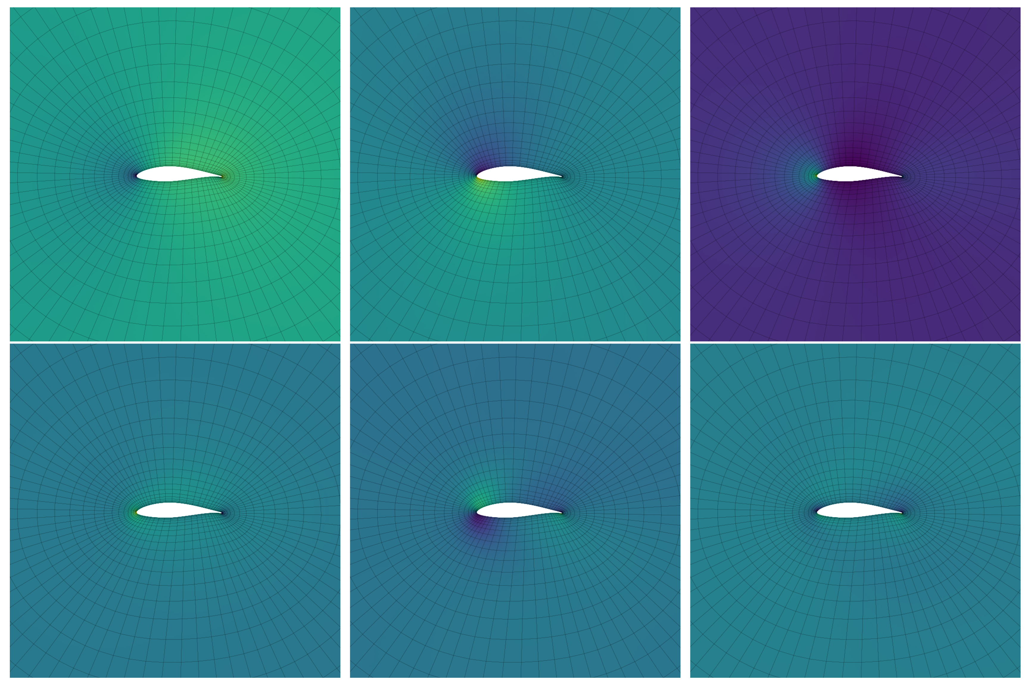
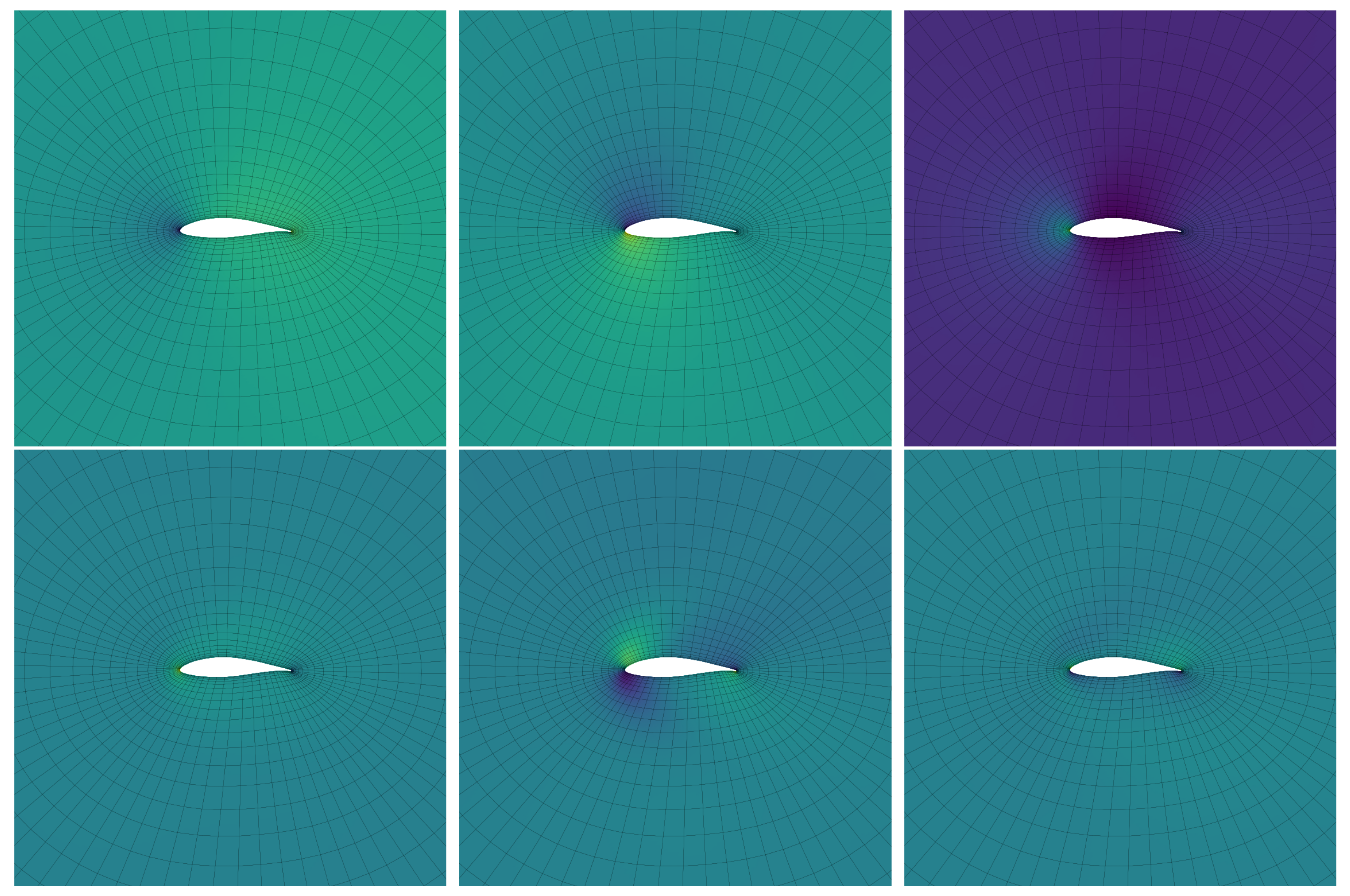
4.3. Spatial Development of Modes/Reduced Basis

To gain insight into the type of eigenmodes we get using POD we display the first six reduced-order basis function for velocities in Figure 7 and Figure 8 and pressures in Figure 9 and Figure 10 obtained with the uniform and mixed ROM methods, respectively. The geometrical variation is highlighted in the modes with vortex fronts of various spatial directions. The POD produces in general optimal linear subspace of modes by acting as an energy filter which identifies the large coherent structures and passes the less coherent structures to the lower modes [46,47]. The figures represent the modes sorted in a hierarchical manner of high to low energetic states of the system with its spatial evolution. All the sorted modes are orthogonal to each other (in respective H 1 -seminorm for velocity and L 2 -norm for pressure) and exhibit a distinct spatial pattern. The change in the spatial distribution of the small coherent structures in the modes is considered to be due to the redistribution of the energy between scales of varying length.
The plots of mixed and uniform reduced methods demonstrate that the first few velocity modes show a mean behavior of the flow field. The first mode, in particular, carries the highest portion of energy and exhibits a mean flow pattern of the velocity field. The second mode exhibits a wake region behind the airfoil; however, the mean behavior is still reflected in it. The third mode interestingly manifests two distinct vortex regions behind the airfoil [48]. These dipole vortex structures turn into tripole structure in the downstream direction of the fourth mode. In the subsequent modes, an addition of one vortex structure is seen in all modes. Increasing vortex structures show the limited coherence of energy in the flow field. The unique large coherent structures are only present in the first few modes, and the lower modes characterize the vorticity structure present inside the flow field. The vorticity mixing and the eddies in the wake are observed to collapse and became less pronounced. The initial modes represent the global behavior (large scale coherent motion), while the following modes have predominantly shown the local response (such as the representation of small eddies in the wake region). For instance, the scales depicted in the corresponding modes principally describes small scales with a subsequent increase in the number of vortices in the wake. Interestingly, the modes from both high-fidelity input methods have shown similar behavior, which demonstrates that irrespective of the input method used, the six first reduced basis functions remain nearly the same.

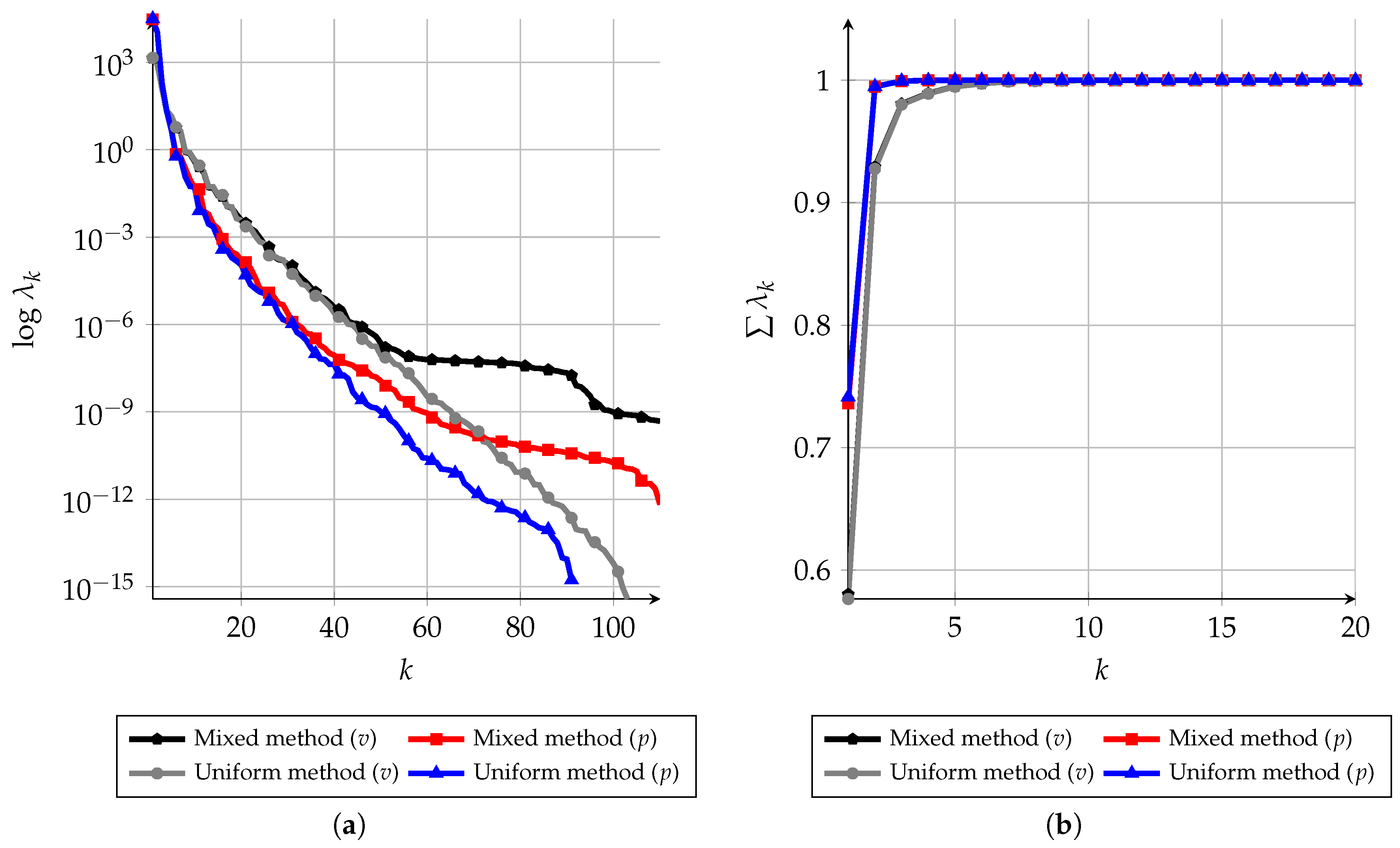
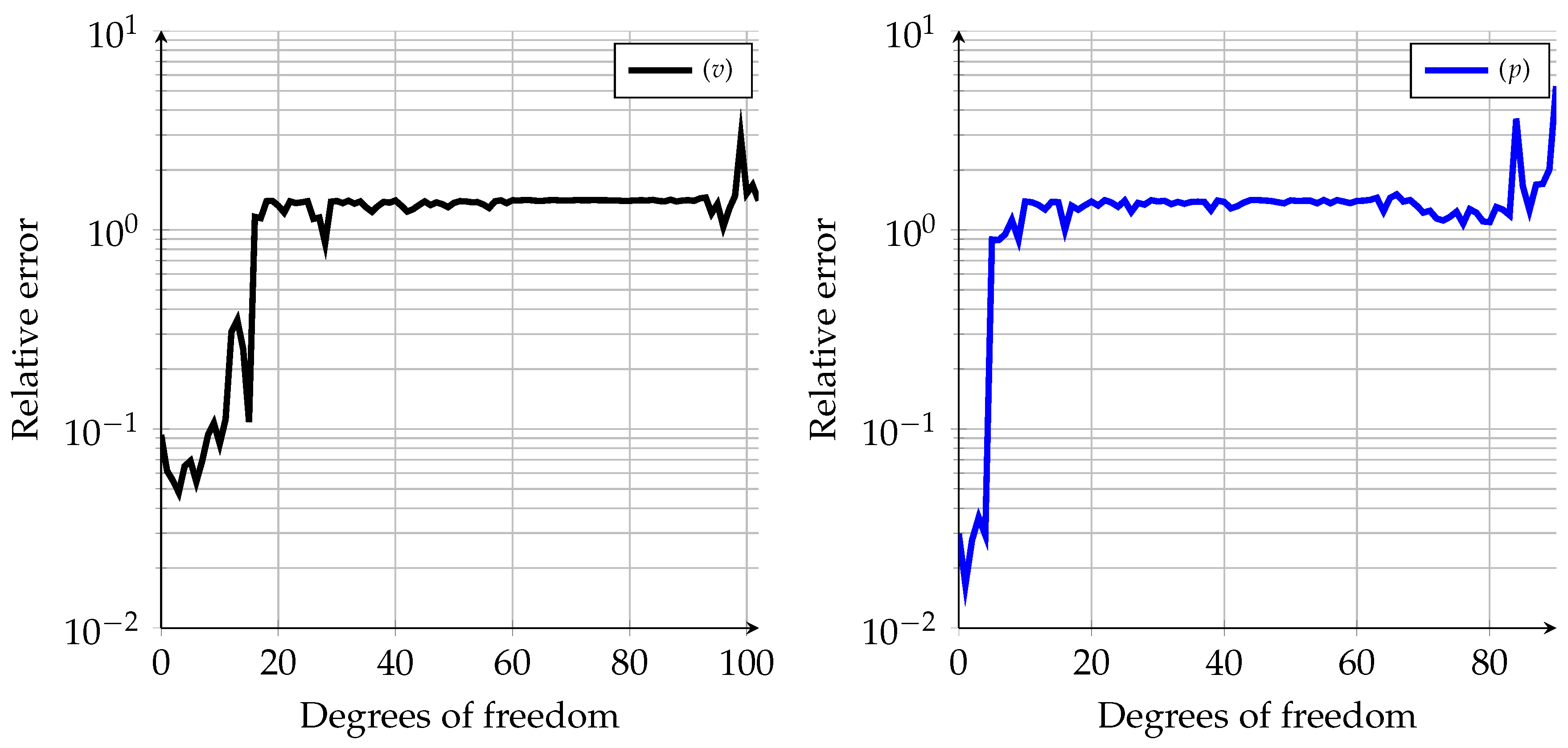
4.4. Spectrum and Related Error

The decay of eigenvalues of the mixed and uniform methods is depicted for the sixty-first modes in the Figure 11a whereas the accumulated energy for the twenty-first modes is shown in Figure 11b and tabulated in Table 1. It highlights the number of basis functions required for a suitable construction of ROM for each method. The decay of energy for velocity is similar for the uniform and mixed method up to the fifty-first modes, whereas, for the scalar pressure, the two methods differ after the forty-first modes.
From Figure 11b we observe that the accumulated energy in the pressure field converges more rapidly towards 1 (i.e., 100%) than correspondingly for the velocity. Table 1 verify this observation. We may expect that the error in H 1 -seminorm for velocity and L 2 -norm is proportional to ϵ if the accumulated energy (measured in the same norms) by the reduced-order modes in the corresponding fields are equal to 1 ϵ 2 [14]. However, Figure 12 shows that the error for pressure does not comply very well with this assertion, only the velocity obtained using the uniform method comply reasonably well. Notice furthermore that the error obtained for the mixed method using nine and more modes is decreasing very slowly (saturation).

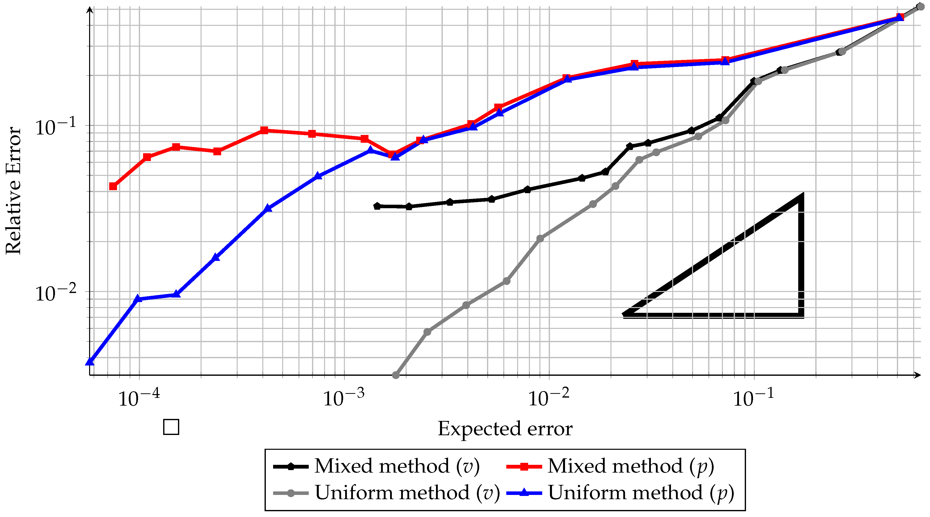
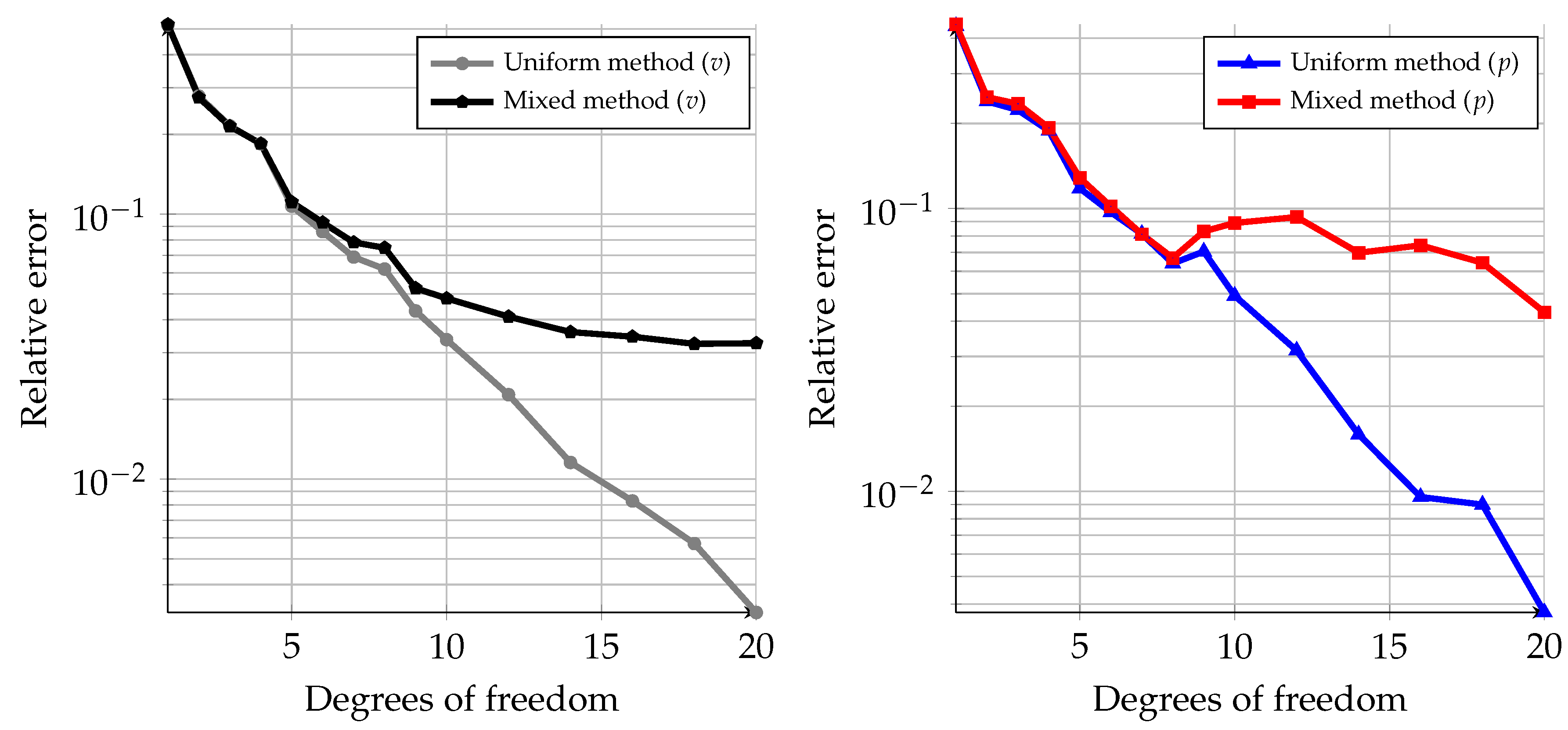
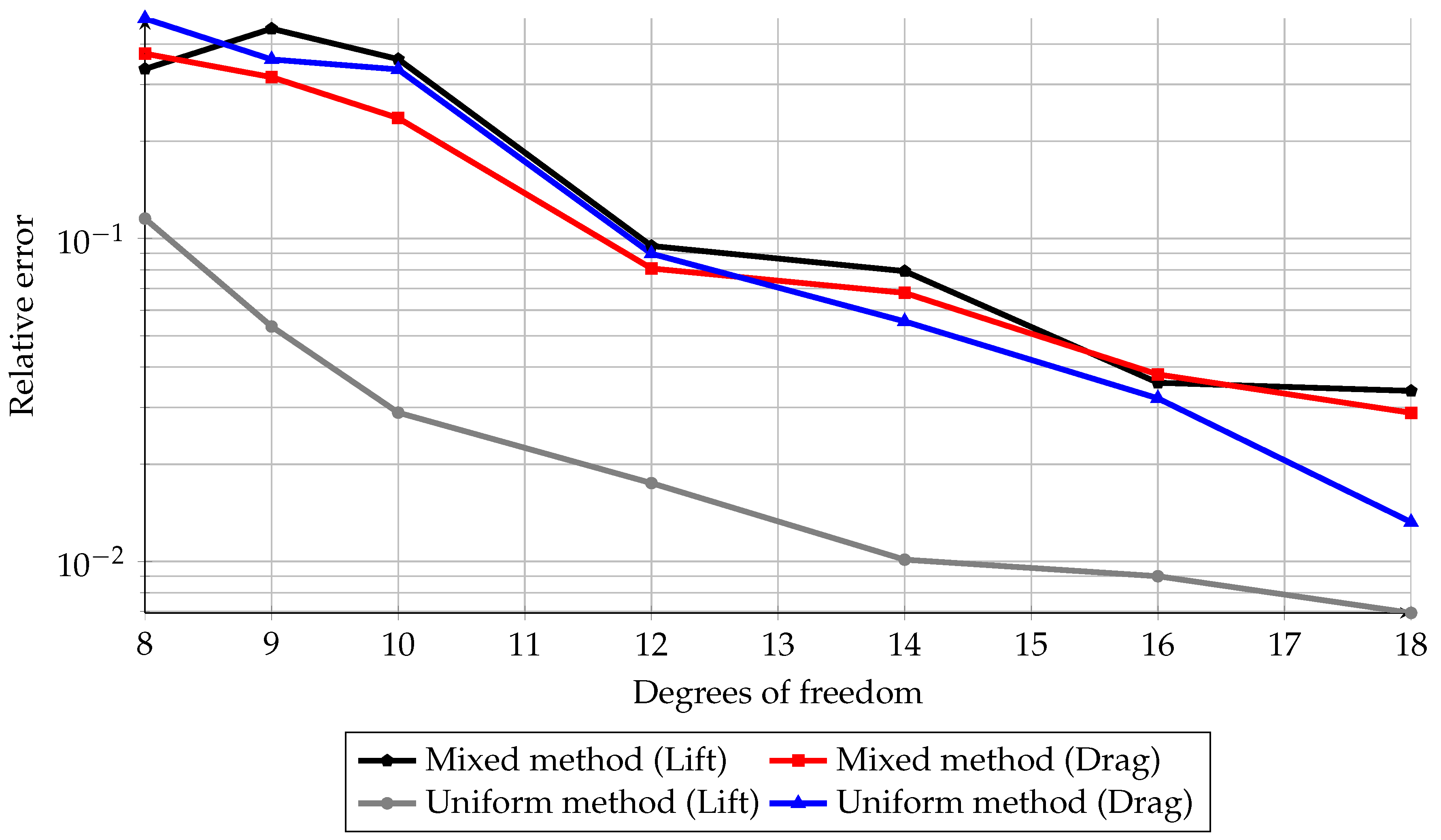
4.5. Accuracy of the Mixed and Uniform Methods

In Figure 13 the relative H 1 -seminorm for velocity and relative L 2 -error for pressure versus the number of reduced-order modes (equivalent to the number of DOFs in the reduced-order model) are displayed. The relative H 1 -seminorm error in the velocity decay rapidly towards 5 % at 5 modes for both the uniform and the mixed methods. The convergence rate for the uniform method is unchanged for a higher number of modes, whereas the mixed method just slowly reduces to 3 % at 20 modes. We observe similar behavior for the relative L 2 -error in the pressure, but here we see a drastic change in convergence rate starting after using 8 modes (with 6 % relative error) and then very slow convergence down to 5 % relative error using 20 modes.
In Figure 14 we have reported the relative error in aerodynamic lift and drag versus DOFs obtained by integrating the tractions derived from the computed reduced-order model solutions. The computed drag is quite similar for the uniform and mixed method, whereas the error in the computed lift is nearly one order lower for the uniform than the mixed method. We see that the relative error in both lift and drag is about 3 % for the mixed method when using 20 modes.
To explain the saturation of the results obtained using the higher number of modes in the mixed method we report in Figure 15 the relative errors between the POD modes obtained from mixed and uniform methods. We clearly see that for velocities the relative error in each POD mode increases steadily up to 18 modes and then flatten outs, whereas for the pressure it flattens out around 8 modes. As the accumulated energy converge rapidly towards unity for the first 10 modes for the velocity and the first 5 modes for pressure the high relative difference in the POD modes higher than 18 and 8 modes for velocity and pressure respectively, results in saturation at acceptable level (i.e., around 3– 5 % relative error in the investigated quantities).
As mentioned in Section 2.2 we must expect an inconsistency error in the mixed method. Even though that the inconsistency error and the error due to the use of a reduced basis are not necessarily orthogonal to each other (in the proper norms) we may expect that relative error of a quantity computed by the presented mixed method to be bounded by the relative difference in the corresponding high-fidelity FE and FV quantity:
ϵ 1 | P | P FE ( μ ) FV ( μ ) FE ( μ )
While the error of the “mixed” methods is bounded, the “uniform” methods continue to converge. However, it must be noted that the errors reported are those between the reduced-order models and the high-fidelity counterparts, which are not necessarily indicative of the true error of the method (as compared to the analytical solution of the PDE). Indeed, one may claim that there is no desire to create reduced models that approximate the high-fidelity model better than that model approximates reality. Since we have that
True ( μ ) ROM ( μ ) True ( μ ) HiFi ( μ ) + HiFi ( μ ) ROM ( μ )
one should aim for the compromise
HiFi ( μ ) ROM ( μ ) True ( μ ) HiFi ( μ )
Assuming that the two methods given the same number of DOFs are comparable in accuracy, one can expect the following a posteriori error estimate to roughly hold.
ROM Uniform ( μ ) ROM Mixed ( μ ) 2 True ( μ ) HiFi ( μ ) .
Given these considerations, it can be seen that the error bound given by Equation (23) does not impose undue problems for “mixed” methods, and that it is only a natural consequence of the reduction process.
In Figure 16, the parametric dependency of the difference between the snapshots generated by the two methods is investigated. It is observed that the differences are not particularly dependent on φ , but that higher differences are reported for slower flows compared to rapid ones. The same behavior is observed in both velocity and pressure norms. An unsymmetrical shape of the profile is observed for the positive and negative values of φ , which is due to the unsymmetrical shape of the airfoil used in the analysis.

4.6. Computational Speedup

The Table 2 illustrates speedups achieved from ROM using the different number of modes (i.e., DOFs). By employing 5 DOF’s, massive speedup of 25,981 is observed for the mixed method, whereas uniform methods show a speedup of 15,370. However, the accuracy is about 10% in relative H 1 -seminorm of the velocity, about 10% in relative L 2 -norm for the pressure and more than 40% relative error in drag and lift. Thus, only 5 reduced-order modes are not acceptable in this case.
If we use 15 modes we observe a speedup of approximately 2000 for the uniform method and close to 3000 for the mixed method. The corresponding relative errors for the four quantities investigated herein are all approximately 5%, which is within the aim for our desired level of accuracy.

5. Conclusions

In this paper, a nonintrusive approach for combining high-fidelity simulations using FV methods with POD and Galerkin Reduced-Order Modeling (ROM) methodology is explored. The key ingredient is to project the FV velocity and pressure results onto suitable FE spaces and then use the classical POD Galerkin ROM framework.
The main finding from our study is that the use of FV high-fidelity snapshots and FE-based ROM, herein denoted mixed method, compute results with an error measured in relative H 1 -norm for the velocity and relative L 2 -norm for the pressure as well as relative error in lift and drag that are all about 5%. The corresponding computational speedup of the mixed method to achieve this level of accuracy was 3000 compared to the FV high-fidelity simulation.
The inherent inconsistency in the mixed method due to the projection of FV results onto the FE Taylor–Hood spaces shows up in higher-order modes but does not preclude the aim of reaching accuracy in the range of 1–10% relative error of the typical quantity of interests for laminar flow problems studied herein.
A natural extension of this work is to develop a mixed method for high Reynolds flow problems, and that will be pursued in future studies.
References

Author Contributions

T.K. and A.R. conceived the research idea. M.S.S. and E.F. performed numerical simulation analyzed data and numerical results. All authors have contributed to the writing, editing, and revising of this manuscript.

Funding

This research was funded by the Norwegian Research Council and the industrial partners of NOWITECH: Norwegian Research Centre for Offshore Wind Technology, OPWIND: Operational Control for Wind Power Plants and FSI-WT: Fluid Surface Interaction of Wind Turbines (Grant No.: 216465) and Norwegian Metacenter for Computational science (NOTUR-reference number: NN9322K/1589).

Conflicts of Interest

The authors declare no conflict of interest.

References

  1. Rui, H. Analysis on a Finite Volume Element Method for Stokes Problems. Acta Math. Appl. Sin. 2005, 21, 359–372. [Google Scholar] [CrossRef]
  2. Luan, S.; Lian, Y.; Ying, Y.; Tang, S.; Wagner, G.J.; Liu, W.K. An enriched finite element method to fractional advection–diffusion equation. Comput. Mech. 2017, 60, 181–201. [Google Scholar] [CrossRef]
  3. Bruger, A.; Nilsson, J.; Kress, W. A Compact Higher Order Finite Difference Method for the Incompressible Navier–Stokes Equations. J. Sci. Comput. 2002, 17, 551–560. [Google Scholar] [CrossRef]
  4. Takizawa, K. Computational engineering analysis with the new-generation space–time methods. Comput. Mech. 2014, 54, 193–211. [Google Scholar] [CrossRef]
  5. Tezduyar, T.E.; Takizawa, K.; Moorman, C.; Wright, S.; Christopher, J. Space time finite element computation of complex fluid structure interactions. Int. J. Numer. Methods Fluids 2010, 64, 1201–1218. [Google Scholar] [CrossRef]
  6. Abbaspour, M.; Radmanesh, A.R.; Soltani, M.R. Unsteady flow over offshore wind turbine airfoils and aerodynamic loads with computational fluid dynamic simulations. Int. J. Environ. Sci. Technol. 2016, 13, 1525–1540. [Google Scholar] [CrossRef]
  7. Bazilevs, Y.; Hsu, M.C.; Akkerman, I.; Wright, S.; Takizawa, K.; Henicke, B.; Spielman, T.; Tezduyar, T.E. 3D simulation of wind turbine rotors at full scale. Part I: Geometry modeling and aerodynamics. Int. J. Numer. Methods Fluids 2011, 65, 207–235. [Google Scholar] [CrossRef]
  8. Bazilevs, Y.; Hsu, M.C.; Takizawa, K.; Tezduyar, T.E. ALE-VMS and ST-VMS methods for computer modeling of wind turbine rotor aerodynamics and fluid-structure interaction. Math. Model. Methods Appl. Sci. 2012, 22, 1230002. [Google Scholar] [CrossRef]
  9. Nayfeh, A.H.; Mook, D.T. Nonlinear Oscillations; Wiley Classic Library Edition: Hoboken, NJ, USA, 1995. [Google Scholar]
  10. Akhtar, I.; Marzouk, O.A.; Nayfeh, A.H. A van der Pol-Duffing oscillator model of hydrodynamic forces on canonical structures. J. Comput. Nonlinear Dyn. 2009, 4, 041006. [Google Scholar] [CrossRef]
  11. Ballarin, F.; Manzoni, A.; Quarteroni, A.; Rozza, G. Supremizer stabilization of POD-Galerkin approximation of parametrized steady incompressible Navier-Stokes equations. Int. J. Numer. Methods Eng. 2015, 102, 1136–1161. [Google Scholar] [CrossRef]
  12. Fonn, E.; Tabib, M.; Siddiqui, M.S.; Rasheed, A.; Kvamsdal, T. A step towards reduced order modelling of flow characterized by wakes using proper orthogonal decomposition. Energy Procedia 2017, 137, 452–459. [Google Scholar] [CrossRef]
  13. Tabib, M.; Rasheed, A.; Siddiqui, M.S.; Kvamsdal, T. A full-scale 3D vs 2.5D vs 2D analysis of flow pattern and forces for an industrial-scale 5MW NREL reference wind-turbine. Energy Procedia 2017, 137, 477–486. [Google Scholar] [CrossRef]
  14. Quarteroni, A.; Manzoni, A.; Negri, F. Reduced Basis Methods for Partial Differential Equations; Springer International Publishing: Berlin, Germany, 2016. [Google Scholar]
  15. Rozza, G. Fundamentals of reduced basis method for problems governed by parametrized PDEs and applications. In Separated Representations and PGD-Based Model Reduction: Fundamentals and Applications; CISM International Centre for Mechanical Sciences; Springer: Berlin, Germany, 2014; Volume 554, Chapter 4. [Google Scholar]
  16. Stabile, G.; Hijazi, S.N.; Lorenzi, S.; Mola, A.; Rozza, G. Advances in reduced order modelling for CFD: Vortex shedding around a circular cylinder using a POD-Galerkin method. arXiv, 2017; arXiv:1701.03424. [Google Scholar]
  17. Hsu, M.C.; Bazilevs, Y. Fluid structure interaction modeling of wind turbines: Simulating the full machine. Comput. Mech. 2012, 50, 821–833. [Google Scholar] [CrossRef]
  18. Soldner, D.; Brands, B.; Zabihyan, R.; Steinmann, P.; Mergheim, J. A numerical study of different projection-based model reduction techniques applied to computational homogenisation. Comput. Mech. 2017, 60, 613–625. [Google Scholar] [CrossRef]
  19. Peng, L.; Mohseni, K. Nonlinear model reduction via a locally weighted POD method. Int. J. Numer. Methods Eng. 2016, 106, 372–396. [Google Scholar] [CrossRef]
  20. Aubry, N. On the hidden beauty of the proper orthogonal decomposition. Theor. Comput. Fluid Dyn. 1991, 2, 339–352. [Google Scholar] [CrossRef]
  21. Ly, H.V.; Tran, H.T. Modeling and control of physical processes using proper orthogonal decomposition. Math. Comput. Model. 2001, 33, 223–236. [Google Scholar] [CrossRef]
  22. Bergmann, M.; Bruneau, C.H.; Iollo, A. Enablers for robust POD models. J. Comput. Phys. 2009, 228, 516–538. [Google Scholar] [CrossRef]
  23. Sirisup, S.; Karniadakis, G. Stability and accuracy of periodic flow solutions obtained by a POD-penalty method. Phys. D Nonlinear Phenom. 2005, 202, 218–237. [Google Scholar] [CrossRef]
  24. Lorenzi, S.; Cammi, A.; Luzzi, L.; Rozza, G. POD-Galerkin method for finite volume approximation of Navier-Stokes and RANS equations. Comput. Methods Appl. Mech. Eng. 2016, 311, 151–179. [Google Scholar] [CrossRef]
  25. Rowley, C. Model reduction for fluids, using balanced proper orthogonal decomposition. Int. J. Bifurc. Chaos Appl. Sci. Eng. 2005, 15, 997–1013. [Google Scholar] [CrossRef]
  26. Bakewell, H.P., Jr.; Lumley, J.L. Viscous sublayer and adjacent wall region in turbulent pipe flow. Phys. Fluids 1967, 10, 1880–1889. [Google Scholar] [CrossRef]
  27. Berkooz, G.; Holmes, P.; Lumley, J.L. The proper orthogonal decomposition in the analysis of turbulent flows. Annu. Rev. Fluid Mech. 1993, 25, 539–575. [Google Scholar] [CrossRef]
  28. Sirovich, L. Turbulence and the dyanmics of coherent structures. Q. Appl. Math. 1987, 45, 561–590. [Google Scholar] [CrossRef]
  29. Noack, B.R.; Eckelmann, H. A low-dimensional Galerkin method for the three-dimensional flow around a circular cylinder. Phys. Fluids 1994, 6, 124–143. [Google Scholar] [CrossRef]
  30. Sirisup, S.; Karniadakis, G.E.; Xiu, D.; Kevrekidis, I.G. Equation-free/Galerkin-free POD-assisted computation of incompressible flows. J. Comput. Phys. 2005, 207, 568–587. [Google Scholar] [CrossRef]
  31. Tallet, A.; Allery, C.; Leblond, C.; Liberge, E. A minimum residual projection to build coupled velocity-pressure POD-ROM for incompressible Navier-Stokes equations. Commun. Nonlinear Sci. Numer. Simul. 2015, 22, 909–932. [Google Scholar] [CrossRef]
  32. Løvgren, A.E.; Maday, Y.; Rønquist, E.M. A reduced basis element method for the steady Stokes problem. ESAIM: M2AN 2006, 40, 529–552. [Google Scholar] [CrossRef]
  33. Jasak, H. Error Analysis and Estimation in the Finite Volume Method with Applications to Fluid Flows; Imperial College, University of London: London, UK, 1996. [Google Scholar]
  34. Prenter, F.; Verhoosel, C.; Zwieten, G.; Brummelen, E. Condition number analysis and preconditioning of the finite cell method. Comput. Methods Appl. Mech. Eng. 2017, 316, 297–327. [Google Scholar] [CrossRef]
  35. Rambo, J.; Joshi, Y. Reduced-order modeling of turbulent forced convection with parametric conditions. Int. J. Heat Mass Transf. 2007, 50, 539–551. [Google Scholar] [CrossRef]
  36. Tezduyar, T. Stabilized Finite Element Formulations for Incompressible Flow Computations; Advances in Applied Mechanics; Elsevier: Amsterdam, The Netherlands, 1991; Volume 28, pp. 1–44. [Google Scholar]
  37. Jain, S.; Bhatt, V.D.; Mittal, S. Shape optimization of corrugated airfoils. Comput. Mech. 2015, 56, 917–930. [Google Scholar] [CrossRef]
  38. Tezduyar, T.; Mittal, S.; Ray, S.; Shih, R. Incompressible flow computations with stabilized bilinear and linear equal-order-interpolation velocity-pressure elements. Comput. Methods Appl. Mech. Eng. 1992, 95, 221–242. [Google Scholar] [CrossRef]
  39. Evans, J.A.; Hughes, T.J.R. Discrete spectrum analyses for various mixed discretizations of the Stokes eigenproblem. Comput. Mech. 2012, 50, 667–674. [Google Scholar] [CrossRef]
  40. Broeckhoven, T.; Smirnov, S.; Ramboer, J.; Lacor, C. Finite volume formulation of compact upwind and central schemes with artificial selective damping. J. Sci. Comput. 2004, 21, 341–367. [Google Scholar] [CrossRef]
  41. Fonn, E.; van Brummelen, H.; Kvamsdal, T.; Rasheed, A. Fast divergence-conforming reduced basis methods for steady Navier–Stokes flow. Comput. Methods Appl. Mech. Eng. 2019, 346, 486–512. [Google Scholar] [CrossRef]
  42. Weller, J.; Lombardi, E.; Bergmann, M.; Iollo, A. Numerical methods for low-order modeling of fluid flows based on POD. Int. J. Numer. Methods Fluids 2010, 63, 249–268. [Google Scholar] [CrossRef]
  43. Couplet, M.; Basdevant, C.; Sagaut, P. Calibrated reduced-order POD-Galerkin system for fluid flow modelling. J. Comput. Phys. 2005, 207, 192–220. [Google Scholar] [CrossRef]
  44. Takizawa, K.; Henicke, B.; Tezduyar, T.E.; Hsu, M.C.; Bazilevs, Y. Stabilized space–time computation of wind-turbine rotor aerodynamics. Comput. Mech. 2011, 48, 333–344. [Google Scholar] [CrossRef]
  45. Takizawa, K.; Tezduyar, T.E. Multiscale space–time fluid–structure interaction techniques. Comput. Mech. 2011, 48, 247–267. [Google Scholar] [CrossRef]
  46. Citriniti, J.H. Reconstruction of the global velocity field in the axisymmetric mixing layer utilizing the proper orthogonal decomposition. J. Fluid Mech. 2000, 418, 137. [Google Scholar] [CrossRef]
  47. Gamard, S.; Jung, D.; Woodward, S.; George, W.K. Application of a slice proper orthogonal decomposition to the far field of an axisymmetric turbulent jet. Phys. Fluids 2002, 14, 2515. [Google Scholar] [CrossRef]
  48. Younis, B.A.; Przulj, V.P. Computation of turbulent vortex shedding. Comput. Mech. 2005, 37, 408. [Google Scholar] [CrossRef]
Figure 1. NACA64: Exaggerated sketch of the domain setup. Solid and dotted lines on the domain boundary represent the Dirichlet boundaries and Neumann boundary condition, respectively. The parameter space consists of a geometrical parameter 25 < φ < 25 and a physical parameter 2   m / s < g < 20   m / s . The mapping π φ represents the transformation between the physical and reference geometry.
Energies 12 01271 g001
Figure 2. NACA64: (a) Each finite element of size 2 h is divided into four finite volumes of size h, and together with bilinear interpolation of the geometry ensures that the geometrical representation of Ω is the same for the FE and FV mesh. (b) Four finite volumes of size h where the dots represent cell-centered velocity and pressure values, the circles represent velocities at the nodes, and squares represents the pressures at the nodes. OpenFOAM produce cell-centered velocities and pressures, whereas the stored velocity and pressure values on the VTK-files are post-processed to cell-vertices (mesh nodes) by means of Inverse Distance Weighting (IDW) and are assumed to vary bi-linearly. (c) A Taylor–Hood FE of size 2 h which have biquadratic interpolation of velocities (circles) and bilinear interpolation of pressure (squares).
Energies 12 01271 g002
Figure 3. NACA64: Schematic of the hexahedral computational mesh used for high-fidelity simulations with φ = π / 4 . The computational domain Ω has a diameter of D = 30   m with a chord length of c = 1   m . G 1 , G 2 , G 3 has N θ = { 60 , 80 , 100 } elements in the angular direction and N r = { 24 , 36 , 44 } elements in the radial direction. G 2 is found to produce a mesh-independent solution. A uniform set of nodes are created around the airfoil ( Γ A ), and similarly around the outer boundary which is circular ( Γ B ). In between corresponding nodes on the airfoil with Cartesian coordinate x A , i and on the outer boundary with Cartesian coordinate x B , i (corresponding points have same angular coordinate) the internal nodes are interpolated using the mathematical expression ( ( ( j / N r ) 3 × x B , i ) + ( ( 1 ( j / N r ) 3 ) × x A , i )), i.e., j are the levels from airfoil (j = 0) to the boundary ( j = N r ), the exponent 3 represents the strength of the mesh grading and N r are the number of elements in the radial direction.
Energies 12 01271 g003
Figure 4. NACA64: The parameter space employed in the analysis consists of the physical parameter 2   m / s < g < 20   m / s and the geometrical parameter 25 < φ < 25 . The training set for finding the reduced-order basis is a uniform tensor product parameter space consisting of 10 × 11 values of the parameters g and φ .
Energies 12 01271 g004
Figure 5. NACA64: θ ( r ) as a function of r. For the mathematical expression see Equation (22).
Energies 12 01271 g005
Figure 6. NACA64: Simulations conducted by (a) steady and the (b) transient solvers under similar operating conditions (conducted using G 2 at ( R e = 20 , g = 20   m / s , φ = 25 )) (c) shows that the two solutions results in differences that are insignificant for our purposes.
Energies 12 01271 g006
Figure 7. NACA64: The first six basis functions for the velocity obtained from the FE-based ROM using the ensemble from FE method. The ensemble solution consists of 110 high-fidelity solutions corresponding to the parameter space of 2   m / s < g < 20   m / s and 25 < φ < 25 . Higher modes represent the global mean behavior of the flow field. Whereas, lower modes show local behavior with increasing vortex fronts and erratic flow distribution with less coherence.
Energies 12 01271 g007
Figure 8. NACA64: The first six basis functions for the velocity obtained from the FE-based ROM using the ensemble from FV method. The ensemble solution consists of 110 high-fidelity solutions corresponding to the parameter space of 2   m / s < g < 20   m / s and 25 < φ < 25 . Higher modes represent the global mean behavior of the flow field. Whereas, lower modes show local behavior with increasing vortex fronts and erratic flow distribution with less coherence.
Energies 12 01271 g008
Figure 9. NACA64: The first six basis functions for the pressure obtained from the FE-based ROM using the ensemble from FV method. The ensemble solution consists of 110 high-fidelity solutions corresponding to the parameter space of 2   m / s < g < 20   m / s and 25 < φ < 25 .
Energies 12 01271 g009
Figure 10. NACA64: The first six basis functions for the pressure obtained from the FE-based ROM using the ensemble from FE method. The ensemble solution consists of 110 high-fidelity solutions corresponding to the parameter space of 2   m / s < g < 20   m / s and 25 < φ < 25 .
Energies 12 01271 g010
Figure 11. NACA64: (a) Velocity and pressure energy spectrum plotted for 60 first modes out of 110 high-fidelity snapshots. The marks are given at intervals of 5 modes. (b) Accumulated energy for the 20 first velocity and pressure modes. The marks are given for the first 10 modes and then in intervals of 2 modes.
Energies 12 01271 g011
Figure 12. NACA64: Relative H 1 seminorm for velocity and relative L 2 error for pressure. Increasing number of modes to the left. The marks are given for the first 10 modes and then in intervals of 2 modes. The triangle represents the assumed correlation rate between expected error and the relative error.
Energies 12 01271 g012
Figure 13. NACA64: Illustration of Error vs degree of freedoms for pressure and velocity for both mixed and uniform methods. The marks are given for the first 10 modes and then in intervals of 2 modes.
Energies 12 01271 g013
Figure 14. NACA64: Relative error of aerodynamic lift and drag error computed as a function of DOFs (i.e., number of modes).
Energies 12 01271 g014
Figure 15. NACA64: Relative error between POD modes obtained from mixed and uniform methods for velocity and pressure. (Relative H 1 seminorm for velocity and relative L 2 error for pressure.)
Energies 12 01271 g015
Figure 16. NACA64: Illustration of the relative FE - FV errors against the parametric space ( φ , g ).
Energies 12 01271 g016
Table 1. NACA64: Accumulated energy for the 20 first velocity and pressure modes.
Mixed-VelocityUniform-VelocityMixed-PressureUniform-Pressure
DoFs i = 1 20 λ i i = 1 20 λ i i = 1 20 λ i i = 1 20 λ i
10.58551454510.57645543850.73347865120.7413536071
20.93206732700.92761878380.99477505760.9948088692
30.98193038850.98014005550.99932054500.9993294807
40.99004005840.98903809800.99985327910.9998502524
50.99542219340.99475466890.99996829220.9999676828
60.99754910110.99715181390.99998271340.9999820036
70.99907814020.99889374200.99999450640.9999940851
80.99938701840.99924432100.99999706400.9999968682
90.99964592980.99955750660.99999842490.9999982012
100.99979086260.99973291710.99999951680.9999994521
110.99988059610.99984914430.99999968610.9999996457
120.99993855750.99991853970.99999983520.9999998220
130.99995602200.99994037280.99999989570.9999998900
140.99997254920.99996168080.99999994270.9999999450
150.99998102900.99997332050.99999996880.9999999681
160.99998926110.99998457070.99999997720.9999999772
170.99999260700.99998917580.99999998430.9999999857
180.99999572570.99999354790.99999998810.9999999904
190.99999695350.99999531220.99999999180.9999999940
200.99999790670.99999681800.99999999450.9999999967
Table 2. NACA64: Illustration for the speed gains for mixed and uniform methods. S p e e d u p is, time taken for high-fidelity divided by the time taken for the reduced solution on average. R e l a t i v e e r r o r is absolute H 1 seminorm error divided by H 1 seminorm of the velocity of the reference/high-fidelity solution.
♯ DoFsSpeedupRelative Error (Velocity)Relative Error (Pressure)
High-fidelity110100
Uniform method515,370 1.0 × 10 1 1.1 × 10 1
104122 3.3 × 10 2 4.9 × 10 2
151972 1.0 × 10 2 1.5 × 10 2
201011 3.1 × 10 3 3.7 × 10 3
Mixed method525,981 1.1 × 10 1 1.2 × 10 1
106902 4.8 × 10 2 8.8 × 10 2
152936 3.5 × 10 2 7.2 × 10 2
201764 3.2 × 10 2 4.2 × 10 2

