Heat Transfer in Latent High-Temperature Thermal Energy Storage Systems—Experimental Investigation

Abstract

Thermal energy storage systems with phase-change materials promise a high energy density for applications where heat is to be stored in a narrow temperature range. The advantage of higher capacities comes along with some challenges in terms of behavior prediction. The heat transfer into such a storage is highly transient and depends on the phase state, which is either liquid or solid in the present investigation. The aim is to quantify the heat transfer into the storage and to compare two different fin geometries. The novel geometry is supposed to accelerate the melting process. For this purpose, a single tube test rig was designed, built, and equipped with aluminum fins. The phase-change material temperature as well as the heat-transfer fluid temperature at the inlet and outlet were measured for charging and discharging cycles. Sodium nitrate is used as phase-change material, and the storage is operated ±30 ${}^{\circ }\mathrm{C}$ around the melting point of sodium nitrate, which is 306 ${}^{\circ }\mathrm{C}$. An enthalpy function for sodium nitrate is proposed and the methodology for determining the apparent heat-transfer rate is provided. The phase-change material temperature trends are shown and analyzed; different melting in radial and axial directions and in the individual geometry sections occurs. With the enthalpy function for sodium nitrate, the energy balance is determined over the melting range. Values for the apparent heat-transfer coefficient are derived, which allow capacity and power estimations for industrial-scale latent heat thermal energy systems.

1. Introduction

Thermal energy storage (TES) systems are widely used to balance between volatile production and consumption of heat. This spectrum reaches from small TES systems for domestic heating or cooling up to high-temperature industrial TES systems with operating temperatures of 400 ${}^{\circ }\mathrm{C}$ or more [1]. Domestic and industrial applications TES systems and electricity production systems can increase the level of use of heat. Storing electricity in the form of heat comes together with the disadvantageous reconversion to electricity based on the carnot-cycle efficiency. This disadvantage does not appear in thermal power plants, when heat is stored before being converted to electricity. All thermal power plants offer a potential field of application for TES systems; among them are the so-called concentrating solar power (CSP) plants.

According to the IRENA Report on Renewable Power Generation Costs 2017 [2], the global levelized cost of electricity for CSP decreased from 0.33 USD/kWh in 2010 down to 0.22 USD/kWh in 2017. The globally installed CSP capacity increased from less than 1 $\mathrm{G}$$\mathrm{W}$ in 2010 to more than $5.6$ $\mathrm{G}$$\mathrm{W}$ in 2017. In 2018, all commissioned CSP plants were equipped with a TES. This has led to an increased installed capacity of TES worldwide in the past year [3]. Combining CSP with TES comes with the important unique selling point of decoupling of electricity generation from the availability of renewable energy in form of solar radiation. New developments of TES technology for CSP are described in [4]. Up to now, only sensible storage systems have been applied to commercial CSP plants. At small scale, a phase-change material (PCM) TES was applied at a Stirling CSP plant in [5]. However, in general, for this purpose, sensible TES systems are among the most widely used types at the moment. An exergy efficiency comparison of high-temperature sensible and latent TES is presented in [6] in which both systems reach similar efficiencies. New concepts also suggest the combination of CSP systems with supercritical $C{O}_2$ power cycles and PCM storage, described in [7]. The use of the solid-solid phase transition of lithium and sodium sulfates mixtures is discussed in [8]; the solid-solid phase-transition enthalpy of these mixtures is comparable to other solid-liquid phase-transition enthalpies.

The topic of using PCM as storage material to use the heat of fusion and increase the storage capacity in a specific temperature range is the driving force behind the so-called latent heat TES. From a scientific point of view, phase-change phenomenon is an important issue, especially but not only in the solid-liquid phase change for TES applications. As Groulx discusses in [9], a huge amount of experimental work exists, but up to now the comparability of those different experiments is needs improvement. The simple comparison of temperature trends is only significant if the thermocouple position, geometry, and other parameters are comparable. What is missing is the description of the storage state, the phase-change state coupled with a measurable quantity, and a performance figure for comparison. This challenge will be discussed in the Materials and Methods section.

A lot of review articles on PCM exist [10,11,12]. Most of them list a huge variety of potential materials, their melting points and the latent heat of fusion. Notable is the smaller number of materials for temperatures higher than 300 ${}^{\circ }\mathrm{C}$ because of limited availability of salts in this temperature range, and the attempt of all authors to address the problem of low thermal conductivities of the PCM, especially in the solid state. Therefore, a lot of numerical and experimental investigations have been published. In recent years, encapsulation and the use of additives have been focused on by parts of the scientific community. Macro-encapsulation is investigated in [13], providing a detailed development strategy for the whole encapsulation process using metal cans. The process is feasible, but costs are still too high for present application. In [14], polytetrafluoroethylene (PTFE) is used as a coating material; thermal and chemical stability for temperatures lower than 350 ${}^{\circ }\mathrm{C}$ were shown. Decreasing the encapsulation size leads to micro-encapsulation with a capsule size less than 1 $\mathsf{\mu }$$\mathrm{m}$. A technique was developed for molten salts; in the specific investigation potassium nitrate served as PCM [15]. Thermal stability and control ability of the process were proven. Nanoparticles may increase the conductivity of PCM, as Hu is demonstrating in [16]; separation effects reduce the positive effect of the particles. The reverse idea is to use aluminum foam with nano-PCM filling. In doing so, the foam can increase the heat-transfer performance; the ratio between the foam and the PCM volume is crucial, as demonstrated in [17]. Other ideas are the direct contact PCM storage in which the PCM and the heat-transfer fluid (HTF) are not separated through a heat exchanger [18], or a screw heat exchanger [19] for keeping the PCM in a transportable state. A good review on transportable PCMs is provided in [20]. Besides the mentioned enhancements of the heat transfer, the most common method is the use of fins. Many experimental investigations are using them because fins are a simple method to increase the surface area and therefore the heat-transfer rate. A sodium nitrate PCM storage was designed and erected in [21] for application in a power plant, equipped with aluminum fins and a storage capacity of 700 $\mathrm{k}$$\mathrm{W}$ $\mathrm{h}$. Other test rigs with finned heat exchanger tubes are described in [22,23]. Using fins comes with two questions: which contour should they have, and how should they be positioned in the storage? To answer these questions, mostly numerical investigations have been carried out using e.g., topology optimization in [24,25]. Different fin positions are focused on in [26] or [27], and fins versus pins are investigated in [28]. The influence of the fin design is shown in [29,30]. Three main findings can be summarized from the mentioned literature. When using fins, an arborescent fin structure shows good results. Then, natural convection plays a role, especially for melting, and finally longitudinally and vertically finned tubes show accumulation of liquid PCM at the top of the storage, in numerical investigations [31] and experiments [23].

Besides the geometry, material compatibility may limit the use of different materials in a PCM storage. As Qiu describes in [32], different stainless steels and their compatibility with NaF-NaCl eutectic salt were examined, and generally low corrosion activity was observed. This is supported by unpublished corrosion tests at the Institute of Energy Systems and Thermodynamics, where different materials (conventional steel, aluminum, and copper) were exposed to liquid sodium nitrate at high temperature. Copper shows significant corrosion rates while aluminum and steel keep the tested weight.

Another topic regarding fins is the mounting on the HTF tube. Probably, the HTF tube material is different to the fin material; the tube may be exposed to high pressure while the fins are supposed to have high heat conductivity. For the actual test rig, the aluminum fins were attached with hinged bolt clamps; for future experiments, bimetallic finned tubes with bending edges will be used as described in [33]. Another mounting technique is clipping, as described in [34]; this promising technology is currently under investigation in an industrial-scale test rig.

For the different enhancement methods, the comparison of models with experiments are common, often with improper assumptions as in [35], where the authors consider conduction as the sole heat-transfer mechanism. The selection of the suitable PCM can be challenging, as Gasia et al. is demonstrating in [36] or Maldonaldo et al. for a higher temperature range between 210 ${}^{\circ }\mathrm{C}$ and 270 ${}^{\circ }\mathrm{C}$ [37]. The influence of the inner heat transfer from the HTF to the tube can also be crucial, as presented in [38]. For low-HTF mass flows, a laminar flow establishes that the heat-transfer coefficient can be lower than on the PCM side of the tube. A good summary of PCM for TES applications is provided in [39].

For the present experimental investigation, a novel fin combination of transversal and longitudinal fins, mounted vertically in a PCM storage, are supposed to be examined. The melting behavior is detected by a higher number of temperature testing points to compare the results qualitatively with numerical investigations mentioned above. Finally, a simple method for describing the enthalpy function of a PCM is presented.

2. Materials and Methods

At this point, the test rig design for the experimental investigation is presented, and the measuring concept and the methodology are explained. The parameters used for the experiments are described, and finally the phase-change model and the heat-transfer coefficient are presented in this section.

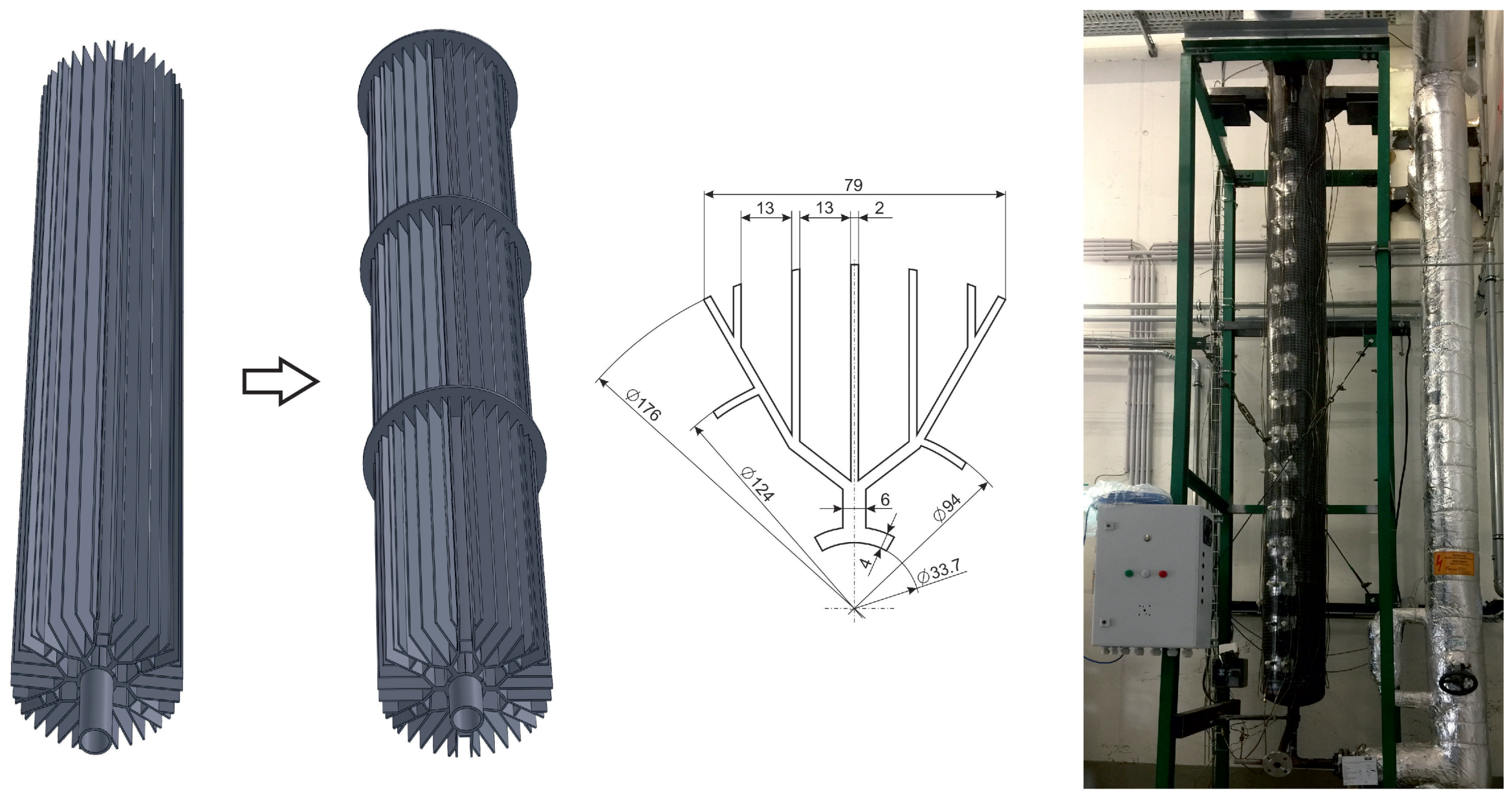
2.1. Test Rig and Testing Point Positions

For the carried-out experiments, a storage test rig was designed and erected at the Institute for Energy Systems and Thermodynamic (IET) at TU Wien, as shown in Figure 1 on the right. As storage material, pure sodium nitrate was selected. The storage vessel is basically a vertical shell-and-tube-design heat exchanger. The inner HTF steel tube is equipped with aluminum fins; between the finned tube and the vessel shell 280 $\mathrm{k}\mathrm{g}$ of PCM was filled in. The storage system is designed as a single tube system; the HTF inlet and outlet are positioned at the bottom and the top of the storage. The vessel has a height of $3.5$ $\mathrm{m}$ where 3 $\mathrm{m}$ is filled with PCM. The outer diameter of the vessel shell is 273 $\mathrm{m}$$\mathrm{m}$; the HTF steel tube has a diameter of $33.7$ $\mathrm{m}$$\mathrm{m}$; the aluminum fins are attached at the steel tube with hinged bolt clamps. Regarding the fins, both transversal and longitudinal fins are applied. The vessel is divided into five sections, within the sections the longitudinal fins are mounted, and the transversal fins mark the borders between the sections. The combination of both fin types is a remarkable novelty compared to former experimental investigations as it is displayed in Figure 2.

A thermal oil plant, as shown in Figure 1 on the left, is used for supplying the test rig with the required heating and cooling power. Therefore, an electric heater with 280 $\mathrm{k}$$\mathrm{W}$_th and a 200 $\mathrm{k}$$\mathrm{W}$_th water-cooler together with mass flow controllers provide a precisely controlled HTF mass flow with temperatures up to 390 ${}^{\circ }\mathrm{C}$. The thermal oil flow direction can be switched by using valves V30–V33 to change the inlet and outlet of the storage. Preliminary work with a comparable storage system [23] showed that the flow direction has an impact on the melting behavior for plain vertical longitudinal fins. When using the novel geometry layout with uniformly distributed transversal fins over a vertical longitudinally finned tube, the flow direction has no effect on the melting behavior anymore, as shown in [40]. Regarding flow direction for the experiments, the direction from the bottom of the storage to the top was chosen.

As shown in Figure 3, temperature testing points are distributed over the whole storage volume in radial and axial direction. The aim was to distribute the temperature testing points uniformly in both radial and axial direction. The temperature is measured with PT100 temperature sensors with an accuracy level AA specified in DIN EN 60751 [41]. For a temperature of 340 ${}^{\circ }$C a deviation of ±0.68 ${}^{\circ }$C is acceptable for this sensor type. In radial direction, the positions $T_a$-$T_d$ are arranged 47 $\mathrm{m}$$\mathrm{m}$, 72 $\mathrm{m}$$\mathrm{m}$, 93 $\mathrm{m}$$\mathrm{m}$ and $136.5$ $\mathrm{m}$$\mathrm{m}$ from the storage axis. This distribution correlates with the radial discretization of the storage volume. The four radial layers are used to calculate the energy balance of the storage. For the radial layers a and b, three testing points per vertical section are installed, for the layers c and d only one testing point per section is available. The axial distances to the subjacent transversal fin are 100 $\mathrm{m}$$\mathrm{m}$, 294 $\mathrm{m}$$\mathrm{m}$ and 488 $\mathrm{m}$$\mathrm{m}$ for $T_a$ and $T_b$. The outer layer testing points $T_c$ and $T_d$ are positioned 400 $\mathrm{m}$$\mathrm{m}$, 1100 $\mathrm{m}$$\mathrm{m}$, 1800 $\mathrm{m}$$\mathrm{m}$ and 2500 $\mathrm{m}$$\mathrm{m}$ from the bottom of the vessel. Besides the PCM temperature, the HTF temperature is measured at the inlet $T_{HTF1}$ and the outlet $T_{HTF2}$ of the storage vessel. For all temperature sensors, a calibration curve was determined by using a temperature dry-well calibrator. Especially for the operation temperature range, the sensors were calibrated precisely to increase the accuracy level. Beside the temperatures, the HTF mass flow is measured with a Proline Prowirl72F from Endress + Hauser Management AG in the secondary loop of the thermal oil plant. This sensor uses a vortex-based measuring principle and has an accuracy of ±1% of the nominal volume flow. The whole plant is equipped with a process control system named APROL from B&R Industrial Automation GmbH. This system allows automatic operation and data acquisition; the examination of the measured data was done with MATLAB.

2.2. Parameter Sets

For a more detailed characterization of the experimental investigation and for repeatability, the parameters in

Table 1. Parameter sets.

Parameter	Symbol	Parameter Set 1	Parameter Set 2
Charging time	$t_{ch}$	6 $\mathrm{h}$	6 $\mathrm{h}$
Discharging time	$t_{dis}$	6 $\mathrm{h}$	6 $\mathrm{h}$
Temperature spread	$\Delta T$	30 ${}^{\circ }\mathrm{C}$	30 ${}^{\circ }\mathrm{C}$
PCM melting temperature	$T_{melt}$	306 ${}^{\circ }\mathrm{C}$	306 ${}^{\circ }\mathrm{C}$
HTF inlet temperature charging	$T_{HTF1}$	336 ${}^{\circ }\mathrm{C}$	336 ${}^{\circ }\mathrm{C}$
HTF inlet temperature discharging	$T_{HTF1}$	276 ${}^{\circ }\mathrm{C}$	276 ${}^{\circ }\mathrm{C}$
HTF mass flow	$\dot{m}$	1 $\mathrm{k}\mathrm{g}$ ${\mathrm{s}}^{-1}$	3 $\mathrm{k}\mathrm{g}$ ${\mathrm{s}}^{-1}$
HTF flow direction	-	$T_{HTF1}$ to $T_{HTF2}$	$T_{HTF1}$ to $T_{HTF2}$

are provided. A latent TES basically is operated around the melting point of the PCM; for the present PCM the melting temperature is 306 ${}^{\circ }\mathrm{C}$. For charging, the HTF inlet temperature is adjusted higher, the difference to the melting point is called the temperature spread $\Delta T$, which is 30 ${}^{\circ }\mathrm{C}$. For discharging, the HTF inlet temperature is controlled to 276 ${}^{\circ }\mathrm{C}$. The HTF mass flow is controlled to either 1 $\mathrm{k}\mathrm{g}$ ${\mathrm{s}}^{-1}$ or 3 $\mathrm{k}\mathrm{g}$ ${\mathrm{s}}^{-1}$, depending on the parameter set. The mass flow represents the only difference between the two sets used in the present investigation. More parameter sets with different temperature spreads and mass flows are provided in [42].

2.3. Phase-Change Material

2.3.1. Modeling the Phase Change

To calculate the energy balance of the storage, the phase change must be described mathematically. In particular, the handling of the latent heat of fusion L is of interest. Theoretically, the PCM melts at its specific melting temperature $T_{melt}$ and during melting no temperature change occurs to the material. From an energy-balance point of view, the specific enthalpy is required and can be written as

$$h\left(T\right)=h_{sens}\left(T\right)+LT\ge T_{melt}.$$

(1)

$h\left(T\right)$ consists of the enthalpy based on the sensible heat and the latent heat of fusion, if the phase change has already happened. Because the temperature in the PCM is measured in non-infinitesimal discretized volumes, the application of L exactly at $T_{melt}$ is not recommended. Around a particular temperature testing point, the PCM shows a heterogeneous temperature distribution. For calculating the energy balance for these specific non-infinitesimal discretized volumes, only one measured temperature is available. Referring to numerical and experimental investigations such as [43], the latent heat of fusion is distributed over a specific melting range. In the present investigation, the lower and upper border are called $T_s$ and $T_l$. The borders are supposed to be chosen in a way that a major part of the PCM in the discretized area is solid when reaching the temperature $T_s$ and reverses for $T_l$. If the PCM is not fully liquid, the enthalpy can be written as follows:

$$h\left(T\right)=h_{sens}\left(T\right)+\gamma \left(T\right)L={\int }_{T_{ref}}^T{c}_{p,sen}\left(T\right)\mathrm{d}T+{\int }_{T_{ref}}^T{c}_p^{*}\left(T\right)\mathrm{d}T={\int }_{T_{ref}}^T{c}_{p,app}\left(T\right)\mathrm{d}T$$

(2)

The liquid fraction $\gamma \left(T\right)$ introduced in Equation (2) is a common quantity to describe the progress of the phase change and has values between 0 for full solidification and 1 for the liquid state. The enthalpy based on the sensible heat $h_{sens}\left(T\right)$ corresponds to the integral of the specific sensible heat capacity of the PCM. The latent heat of fusion $L\left(T\right)$ distributed over a temperature range is defined as equivalent specific heat capacity for the melting range, called $c_p^{*}$. The correlation between $c_p^{*}$ and the liquid fraction is

$$\gamma \left(T\right)=\frac{{\int }_{T_{ref}}^T{c}_p^{*}\left(T\right)}{L}.$$

(3)

Furthermore, the apparent specific heat capacity $c_{p,app}$ is introduced. The apparent specific heat capacity is a combination of the specific heat capacity and the latent heat of fusion. It is possible to compare this function directly with physical measurements of the specific heat capacities and the latent heat of fusion. Differential scanning calorimetry (DSC) is the most common measurement method to determine these values, as described in [44]. Attention must be paid to the heating rate, as it has a direct influence on the determination of the melting temperature. Lower heating rates lead to more accurate melting temperatures; the heat of fusion and the melting point must be determined separately. Anyway, the result of such heat capacity measurements is a heat capacity function over time as provided in [45,46]. For the present model, the specific heat capacity is described with three functions.

$$c_{p,sen}\left(T\right)=\left\{\begin{array}{cc}{c}_{p,s}\left(T\right)\hfill & T_{lrv}\le T<T_s\hfill \\ c_{p,m}\left(T\right)\hfill & T_s\le T\le T_l\hfill \\ c_{p,l}\left(T\right)\hfill & T_l<T\le T_{urv}\hfill \end{array}\right.$$

(4)

One for the solid temperature range, one for the liquid temperature range, and one for the melting range. The melting-range function is a simple linear interpolation between the specific heat capacity $c_{p,s}\left(T_s\right)$ for the solid range and $c_{p,l}\left(T_l\right)$ for the liquid range. The solid and liquid heat capacity function can be determined with DSC measurements; in most cases, fitted linear functions seem to be adequate. Additional to the specific heat capacity, the latent heat of fusion can be described by using the equivalent specific heat capacity with a fourth-grade polynomial.

$$c_p^{*}\left(T\right)=a{T}^4+b{T}^3+c{T}^2+dT+e{T}_s\le T\le T_l$$

(5)

Attention must be drawn to the fact that the equivalent specific heat capacity is defined only in the melting range; for the solid and the liquid range it is supposed to be zero. In earlier numerical investigations such as [43], the liquid fraction $\gamma$ is approximated with an error function. To simplify the handling of the used functions and to increase the performance, a simple fourth-degree polynomial was applied as equivalent specific heat capacity $c_p^{*}$ function. The advantage is based on the fact that the $c_p^{*}$ function can be integrated and derived easily to calculate the liquid fraction and to determine the specific enthalpy. The boundary conditions satisfied by the $c_p^{*}\left(T\right)$ polynomial can be summarized as follows:

$$\begin{array}{cc}\hfill c_p^{*}\left(T_s\right)& =0\hfill \end{array}$$

(6)

$$\begin{array}{cc}\hfill c_p^{*}\left(T_l\right)& =0\hfill \end{array}$$

(7)

$$\begin{array}{cc}\hfill {\left.\frac{\mathrm{d}{c}_p^{*}}{\mathrm{d}T}\right|}_{T_s}& =\frac{\mathrm{d}{c}_{p,s}\left(T_s\right)}{\mathrm{d}T}-\frac{\mathrm{d}{c}_{p,m}\left(T_s\right)}{\mathrm{d}T}\hfill \end{array}$$

(8)

$$\begin{array}{cc}\hfill {\left.\frac{\mathrm{d}{c}_p^{*}}{\mathrm{d}T}\right|}_{T_l}& =\frac{\mathrm{d}{c}_{p,m}\left(T_l\right)}{\mathrm{d}T}-\frac{\mathrm{d}{c}_{p,s}\left(T_l\right)}{\mathrm{d}T}\hfill \end{array}$$

(9)

$$\begin{array}{cc}\hfill {\int }_{T_s}^{T_l}{c}_p^{*}\mathrm{d}T& =L\hfill \end{array}$$

(10)

The boundary conditions ensure that the apparent specific heat capacity function is continuous (conditions (6) and (7)) and is continuously differentiable over the whole range of application (conditions (8) and (9)). Condition (10) ensures that the area under $c_p^{*}$ is equivalent to the latent heat of fusion. With the boundary conditions, the polynomial coefficients in Equation (5) can be determined by solving a simple linear system of equations. Finally, the apparent specific heat capacity $c_{p,app}$ and the enthalpy function $h\left(T\right)$ can be described with simple polynomial functions which can be easily implemented for different PCMs. The application of the above-mentioned procedure is provided in the following subsection for sodium nitrate.

2.3.2. Sodium Nitrate

In the present experimental investigation, pure sodium nitrate (NaNO${}_3$) serves as PCM. Literature references for the melting point $T_{melt}$ and the latent heat of fusion L can be found in [47]. The mentioned values are used for calculating the enthalpy function of sodium nitrate as mentioned above and are listed in

Table 2. Properties and boundary values of sodium nitrate for the specific enthalpy function.

Description	Symbol	Value
Melting temperature	$T_{melt}$	306 ${}^{\circ }\mathrm{C}$
Latent heat of fusion	L	$179.8$$\mathrm{k}$$\mathrm{J}$$\mathrm{k}\mathrm{g}$−1
Solidification temperature limit	$T_s$	300 ${}^{\circ }\mathrm{C}$
Liquidation temperature limit	$T_l$	312 ${}^{\circ }\mathrm{C}$
Enthalpy reference temperature	$T_{ref}$	0 ${}^{\circ }\mathrm{C}$
Lower range of validity	$T_{lrv}$	0 ${}^{\circ }\mathrm{C}$
Upper range of validity	$T_{urv}$	400 ${}^{\circ }\mathrm{C}$

. The melting temperature range was chosen with ± 6 ${}^{\circ }\mathrm{C}$ around the melting point. Range of validity 0 ${}^{\circ }\mathrm{C}$ to 400 ${}^{\circ }\mathrm{C}$ was assumed since this range covers the entire operation temperature range of the storage. Furthermore, specific heat capacity data is available for the mentioned range.

After specifying the properties and boundary values, the functions for the specific heat capacity for the different temperature ranges must be determined. For sodium nitrate, they are proposed as follows:

$$c_{p,sen}\left(T\right)=\left\{\begin{array}{c}{c}_{p,s}\left(T\right)=0.003214T+0.9262\hfill \\ c_{p,m}\left(T_{cen}\right)=-0.02T_{cen}+1.8904\hfill \\ c_{p,l}\left(T\right)=1.65\hfill \end{array}\right.$$

(11)

The function for the solid range $c_{p,s}\left(T\right)$ is based on DSC measurements in [45]. A linear fit for the $c_p$ values seemed to be acceptably exact and led to the mentioned formulation. For the liquid phase, the value from [47] was chosen and crosschecked with the DSC measurements. For the melting range, a linear fit between $c_{p,s}\left(T_s\right)$ and $c_{p,l}\left(T_l\right)$ centered at $T_s$ led to the $c_{p,m}\left(T_{cen}\right)$ function. According to Equation (2), the latent heat of fusion can be expressed based on the equivalent specific heat capacity in the form of Equation (5):

$$c_p^{*}\left(T_{cen}\right)=0.0216147T_{cen}^4-0.518730T_{cen}^3+3.110310T_{cen}^2+0.0232473T_{cen}$$

(12)

The polynomial is centered at $T_s$:

$$T_{cen}=T-T_s$$

(13)

In Figure 4 the individual functions are compared with measurements from [45]. Focusing on the function $c_{p,s}$ for the solid temperature range, the experimental data show a solid-solid phase transition at 276 ${}^{\circ }\mathrm{C}$. This phase transition is not reproduced in the simple linear approximation because the cyclic operation temperature is higher. For the melting zone, the specific heat capacity consists of the sensible $c_{p,m}$ and the equivalent specific heat capacity $c_p^{*}$. Both together form a peak similar to the experimental data, but the peak is shifted to 306 ${}^{\circ }\mathrm{C}$ in the model. This difference may be a result of the heating rate during the DSC measurement. To fulfill the physical specification of the melting point, the shifting seems to be acceptable. The heights of the peaks are similar; in the model it depends mainly on the melting-range temperatures and the latent heat of fusion. This method can be easily adapted for other materials when the enthalpy of fusion and the melting point are known.

To determine the enthalpy function, the $c_{p,app}$ function must be integrated. Compared to other approaches, the polynomial functions can be integrated without great effort. The reference temperature is 0 ${}^{\circ }\mathrm{C}$ for the present investigation. The enthalpy function $h\left(T\right)$ persists of three individual polynomial functions for the solid, the melting, and the liquid temperature range. With this enthalpy function, the energy balance of the TES in Section 3.5 was calculated.

A comparison of the polynomial approach with the error function approach in [43] is provided in Figure 5. The liquid fraction applied for sodium nitrate shows a similar trend; the polynomial approach has slightly different gradients, compared to the error function.

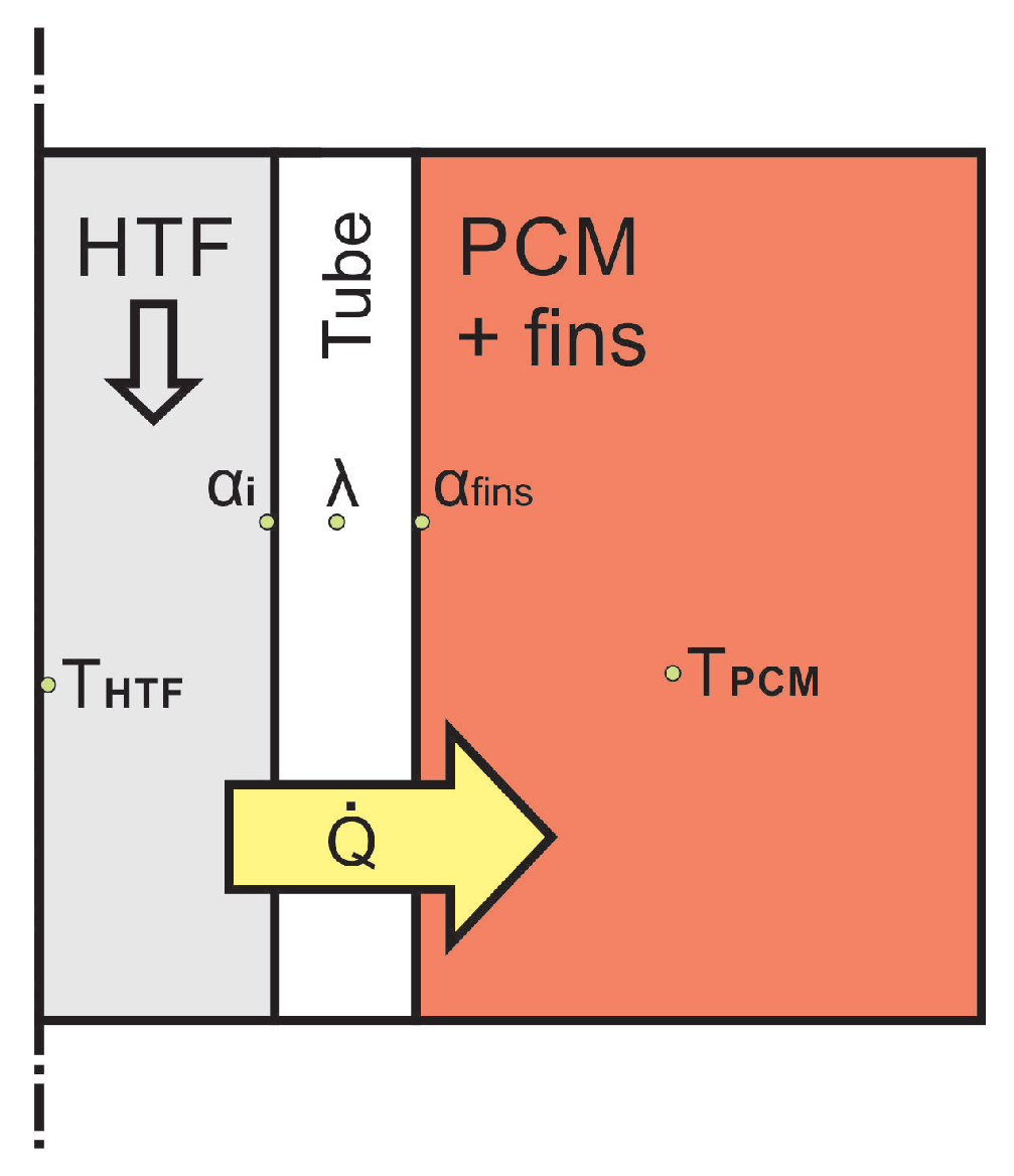
2.4. Heat Transmission from the HTF into the PCM

To describe the heat transmission from the HTF into the PCM, a scheme is presented in Figure 6. In the steel tube, the HTF temperature is measured at the inlet $T_{HTF1}$ and the outlet $T_{HTF2}$. A mean HTF temperature can be determined. From the HTF to the steel tube, an inner heat-transfer coefficient ${\alpha }_i$ was calculated as described in [48] for a flow in a tube, depending on the velocity and the HTF properties. For the experimental setup, the flow was turbulent with Reynolds numbers greater than 2300. The material properties of the HTF were taken from the manufacturer data-sheet [49]. The heat conduction in the steel tube can be calculated straightforwardly. For the heat transfer on the outer side of the steel tube, an apparent heat-transfer coefficient ${\alpha }_{fins}$ is introduced. It mainly depends on the fin geometry and the phase-transition state, which must be considered for the values provided in the results section.

On the PCM side, a mean storage temperature is introduced. The radial discretization of the PCM into four circular rings, together with the measured temperatures at the element borders, allow calculation of the weighted average temperature:

$$T_{PCM}=Tm=\frac{{\sum }_{j=a}^d{T}_j{m}_j}{m_{PCM}}$$

(14)

The heat flux can be calculated as follows:

$$P_{HTF}=\dot{m}\left[h_{HTF}\left(T_{HTF1}\right)-h_{HTF}\left(T_{HTF2}\right)\right]$$

(15)

For the heat conduction in a cylinder with the length l and one layer provided in [48], the heat flux can be written as:

$$P_{HTF}=\frac{2\pi (T_{HTF}-Tm)}{\frac{1}{r_i{\alpha }_i}+\frac{1}{2{\lambda }_{steel}}ln\left(\frac{r_i}{r_o}\right)+\frac{1}{r_o{\alpha }_{fins}}}$$

(16)

Assuming that ${\alpha }_{fins}$ can be determined now, the exact trend is provided in the result section. Values for the inner heat transmission ${\alpha }_i$ coefficient vary between 1000 and 4000 $\mathrm{W}$ $\mathrm{m}$${}^2$ $\mathrm{K}$ for the different mass flows of 1 $\mathrm{k}\mathrm{g}$ ${\mathrm{s}}^{-1}$– 3 $\mathrm{k}\mathrm{g}$ ${\mathrm{s}}^{-1}$ and the different HTF temperatures. For the heat conduction coefficient of steel ${\lambda }_{steel}$, 50 $\mathrm{W}$ ${\mathrm{m}}^{-1}$ $\mathrm{K}$ was chosen. This value has no significant influence on the overall heat transmission. Values for ${\alpha }_{fins}$ are in the range of 300 $\mathrm{W}$ $\mathrm{m}$${}^{-2}$ to 1500 $\mathrm{W}$ $\mathrm{m}$ ${}^{-2}$, depending on the mean storage temperature. For the case of low-HTF velocities, the inner heat-transfer coefficient can become much lower so the inner heat-transfer could become the crucial value. With the measured values for the apparent heat transfer on the outer side of the steel tube, an extrapolation to similar geometries and higher storage capacities can be done and the power trend for comparable storage types can be predicted. Up-scaling the actual lab-scale test rig to industrial-scale TES is viable.

3. Results

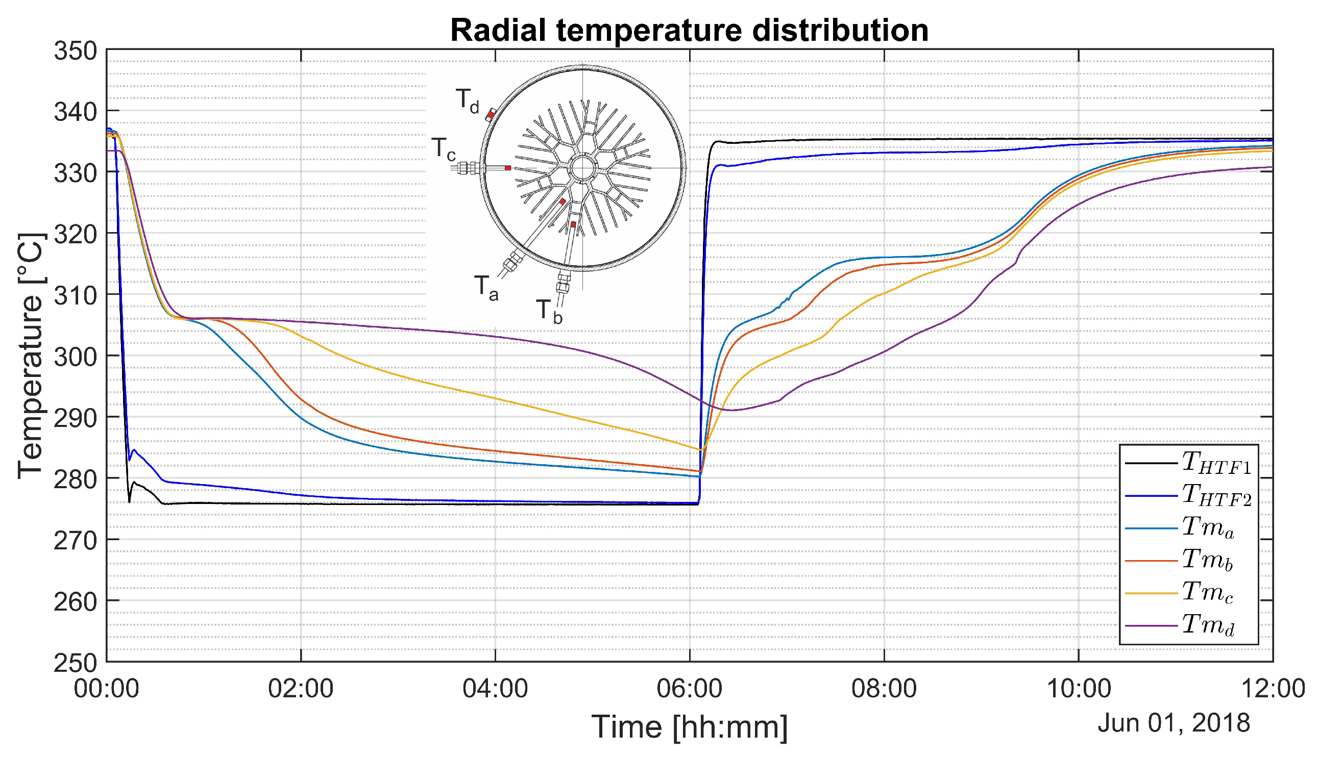
3.1. Temperature Distribution in the Storage with the Combination of Transversal and Longitudinal Fins

The temperature distribution in the PCM is measured in four mean radial positions ($T{m}_a$-$T{m}_d$). Figure 7 shows their temperature trend. From this data, a typical temperature trend for TES with PCM can be deviated, especially for discharging, which takes place from 0 to 6 $\mathrm{h}$. The temperature gradient at the melting temperature of the PCM ( 306 ${}^{\circ }\mathrm{C}$) is zero; in this period, the phase change occurs at the specific measuring point. The phase-change time increases for the outer positions ($T{m}_c$ and $T{m}_d$) due to more PCM mass. For charging, this effect cannot be seen so clearly, especially looking at positions $T{m}_c$ and $T{m}_d$. A possible explanation for these results may be the stronger natural convection in the liquid PCM during melting in this region. It is possible that the finned area ($T{m}_a$ and $T{m}_b$) limits natural convection, and therefore the melting point can be seen more clearly in this trend. This effect is supported by the results of numerical investigations in which fins hinder the flow of the liquid PCM [50]. The melting and solidification starts from the inside and moves to the outer shell. Interestingly, the process velocity differs, while for melting, the temperature $T{m}_d$ converges to a stationary value after six hours. It is not stationary after six hours of discharging. The solidification process of the PCM takes more time than the melting, which confirms numerical simulation as in [29] and former measurements as in [23].

In the axial direction, the vessel is split into five vertical sections by transversal fins. These sections are equipped with different measuring points to examine the uniformity of distribution within the sections but also over the total height of the storage. Therefore, the temperatures within the sections are averaged and displayed in Figure 8. The mean temperatures in the particular sections do not spread much. Interestingly, the temperatures $T{m}_1$ and $T{m}_5$ have the highest deviation; all others show a uniform trend. It is not difficult to explain this behavior, since the two temperatures represent the lower and upper end of the vessel. Boundary conditions such as the difference in insulation or the air layer in Section 5 over the PCM are likely reasons for the deviation. The vessel is mounted to a steel construction at the top of Section 5 (see Figure 2), so the insulation differs to other sections. Nonetheless, these results indicate a uniform temperature distribution over the whole vessel in axial direction, which is contrary to former experimental investigations with plain longitudinal vertical fins [23].

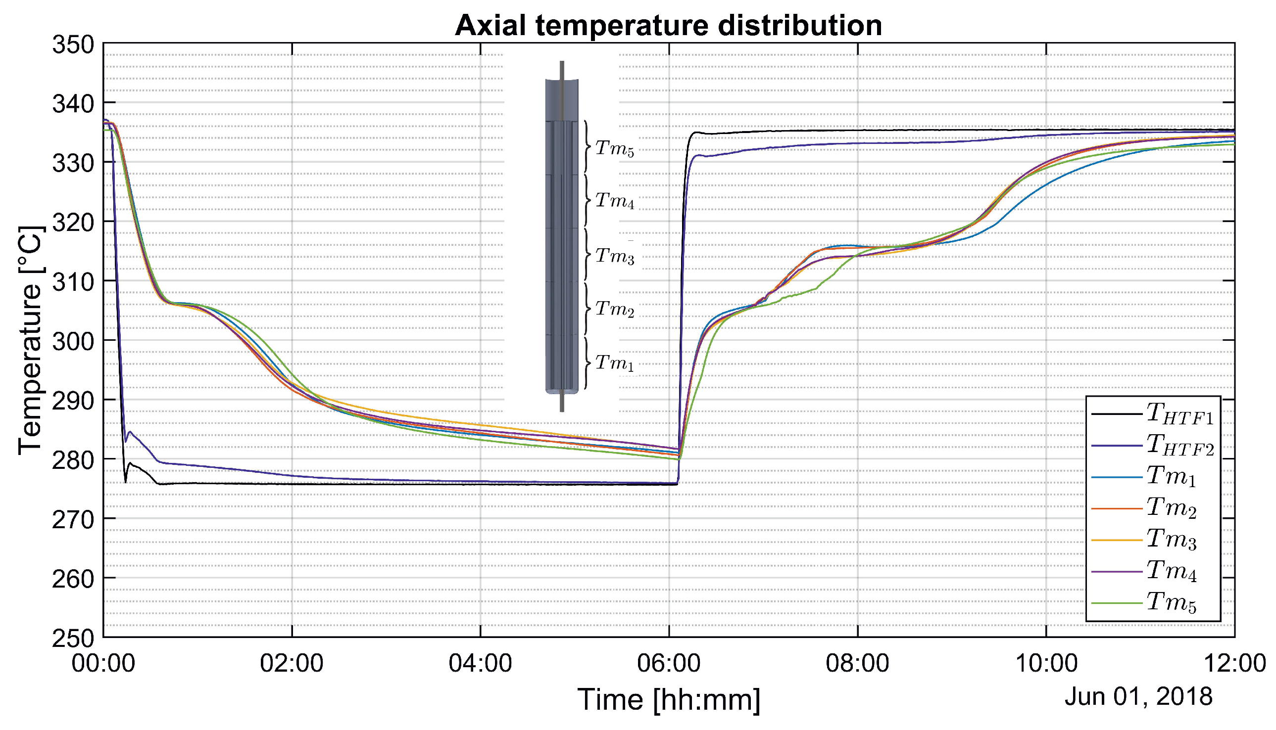
3.2. Axial Temperature Distribution in a Vertical Section

Another important finding is that the axial temperature distribution on a local level is different to the global axial distribution mentioned above. In each section, the temperature is measured in different heights and different radial distances. Therefore, in the position $Ta$ three measuring points exist in each section, for example $T{a}_{3\_2}$ is the middle one in the third section in the radial position a. Out of the five sections, the mean temperature for the three axial positions in one section were calculated and are presented in Figure 9. From the graph, it can be seen that the temperatures are mostly uniform beside the time from 7 to $9.5$ $\mathrm{h}$. In this period the PCM temperature is in a range of 306 to 325 ${}^{\circ }\mathrm{C}$ and the PCM is in the liquid phase. Furthermore, the temperature gradient between the PCM and the HTF is high; hot and liquid PCM accumulates at the top of each section. Natural convection plays a non-negligible role in the heat-transfer mechanism during melting, as previously described by Walter in [29]. For solidification, the axial temperature distribution is uniform, heat conduction is the dominating and limiting factor for the heat transmission. However, findings of the current experimental investigation support the previous numerical simulations.

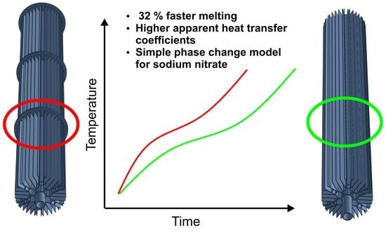
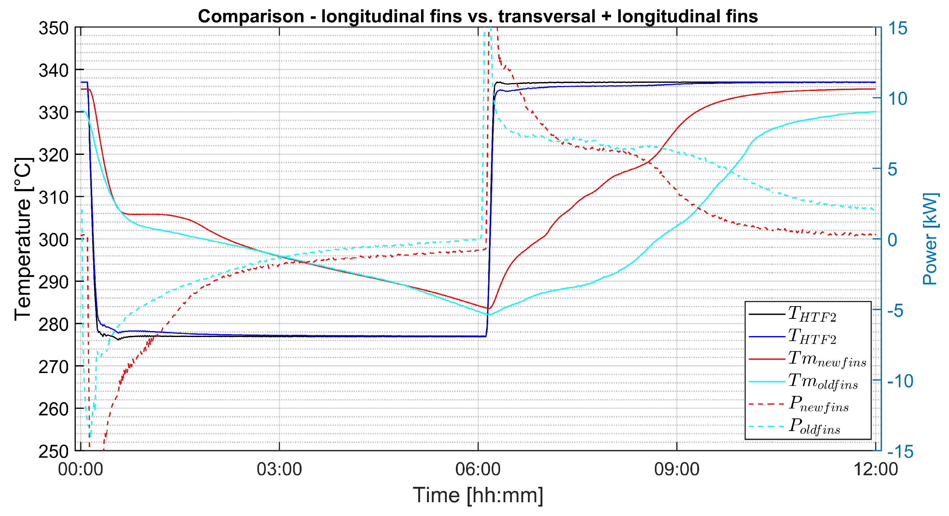
3.3. Comparison of Different fin Geometries

A prior experimental investigation with a comparable test rig but plain vertical longitudinal fins was carried out in 2017. To compare the effectiveness of the two different fin types, the mean storage temperature and the power rate is presented in Figure 10. It is apparent that the mean storage temperature trend $Tm$ while discharging is similar for both fin types. The plain longitudinal fins seem to be a little bit faster, but the maximum storage temperature therefore is lower. A significant difference can be observed while charging; $T{m}_{newfins}$ has a higher gradient and reaches a higher level. 325 ${}^{\circ }\mathrm{C}$ of mean storage temperature reached 32% faster with the new fin type. Turning now to the power rate, a significant difference can be observed for both charging and discharging. During solidification, the power rate is consequently higher with the new fin type. Interestingly, the charging process can be completed much faster, the mean storage temperature reaches a higher level faster, and then the power rate decreases rapidly (from 9 to 10 $\mathrm{h}$).

3.4. Apparent Heat-Transfer Coefficient ${\alpha }_{fins}$

The heat transmission from the HTF into the PCM or the reverse can be split up into different sub-areas and effects. In the HTF tube, the heat-transfer coefficient ${\alpha }_i$ from the fluid to the wall depends mainly on the fluid velocity and material properties. For the steel tube, heat conduction normally is high compared to the PCM. On the outer side of the steel tube, an apparent heat-transfer coefficient ${\alpha }_{fins}$ can be determined. This parameter is valid for the specific geometry and material combination and is presented in Figure 11. In the chart, the apparent heat-transfer coefficients for the two different fin geometries are compared. It can be seen that the value for the new fin type is significantly higher than the other one, especially in the more important first three hours of charging and discharging. As can be seen in Figure 10, the mean storage temperature for the new fins and charging approaches an asymptotic temperature after 9 $\mathrm{h}$. That means that the storage is almost charged after half the charging time. The temperature difference between inlet and outlet becomes small and the values for ${\alpha }_{fins}$ spread, as can be seen in Figure 11. Summing up, the heat-transfer coefficients are essential for the duration of charging and discharging but not for the asymptotic steady state.

3.5. Energy Balance—Capacities and Losses

Turning now to the energy balance of the storage vessel, Figure 12 provides energy and power trends to compare the stored energy from an HTF-based perspective with an PCM-based perspective. The HTF temperatures at the inlet and outlet ($T_{HTF1}$ and $T_{HTF2}$) together with the measured mass flow result in the power which is displayed as a black dashed line. Integration of the HTF-based power gives the energy, a black full line in the chart. The storage consists of the PCM, a steel vessel, and aluminum fins. Furthermore, losses will appear in the energy balance, based on the insulation thickness, storage temperature, and the cycle time. The temperatures for all components are measured, integrated over the time, and, together with the different enthalpies, the energy for the whole storage can be presented ($E_{storage}$, the red full line). This energy consists of the particular energy expression for the steel, aluminum, and the losses. Complying with the energy balance means that the red and the black lines are supposed to have the same trend and end up at the same value after a cycle. Interestingly, for charging, the two lines have a similar trend, and the deviation is low. For discharging, the trends show a higher deviation. The difference in energy between storage- and HTF-based calculations at the end of charging/discharging is relatively low for experimental investigations. Several limitations may affect the trend. One is the fault tolerance of the thermocouples in the HTF and the mass flow sensor. Another one is the limited radial temperature resolution to four sensor layers ($T_a$ to $T_d$). Therefore, the temperature distribution in the PCM is probably not detailed enough. The PCM-stored energy is the biggest share, so the PCM temperature has a significant influence on the energy. Steel and aluminum masses do not play a huge role in the energy balance and the losses mainly depend on the insulation thickness. For a more detailed picture, the PCM temperature distribution must be measured with a higher resolution—more radially distributed thermocouples.

4. Discussion

Focusing on the radial temperature trends in Figure 7, it can be summarized that naturally the melting occurs radially from the inside to the outside. For the positions $T{m}_a$ and $T{m}_b$ in the finned zone, the melting and solidification happens faster for the outer testing points $T{m}_c$ and $T{m}_d$. From a global axial perspective, the mean temperatures in the particular sections do not diverge much in Figure 8; axial uniformly melting occurs. Looking at one individual section in Figure 9, the temperature at the top of the section is higher than at the bottom. The non-uniform temperature distribution over the whole storage in [23] can only be observed now in the individual sections. For a comparison of the two different fin geometries, the mean storage PCM temperature $Tm$ was calculated for both in Figure 10. A 32% faster melting can be seen. The power rate for the novel fin geometry is consequently higher with the new fin type. Regarding the heat-transfer coefficient ${\alpha }_{fins}$ in Figure 11, higher values can be obtained throughout the cycle. Melting and solidification of the PCM and the heat transfer are highly transient processes, so the heat-transfer coefficient at the outer diameter of the HTF steel tube, as described in the methods sections above, can be stated as a function from the mean PCM temperature in the storage. Therefore, average values between 400 $\mathrm{W}$ ${\mathrm{m}}^{-2}$ ${\mathrm{K}}^{-1}$ for the solid PCM and 1500 $\mathrm{W}$ ${\mathrm{m}}^{-2}$ ${\mathrm{K}}^{-1}$ for the liquid PCM can be expected for the present configuration. Based on that values, the TES behavior can be predicted for utility scale TES systems with the fin geometry proposed in this investigation. Therefore, the inner heat transfer in the tube cannot be neglected. For low flow velocities, this value can become critically low, but compared to the heat transfer from the tube to the PCM, numerical correlations are available. Finally, the energy balance for the whole storage system was determined to examine the validity of the results in Figure 12. The losses to the surrounding as well as the heat capacities of the aluminum and the steel were considered. Together with the heat capacity of the PCM and the measured temperatures, the delivered heat from the HTF fluid can be compared with the temperature rise in the PCM, aluminum, and steel. The deviation between $E_{HTF}$ and $E_{Storage}$ can be interpreted as measurement deviations and deviations based on the discretized resolution of the temperature testing points. The fit between the two curves is satisfying considering the experimental setup behind the data and it seems to be physically plausible. Again, the main findings:

• The combination of transversal and longitudinal fins leads to global axially symmetric melting.
• The combination of transversal and longitudinal fins leads to 32% faster melting compared to plain longitudinal fins.
• Apparent heat-transfer coefficients between 400 and 1500 $\mathrm{W}$ ${\mathrm{m}}^{-2}$ ${\mathrm{K}}^{-1}$ could be determined
• A simple method for the enthalpy function of sodium nitrate in the melting range is presented, based on an apparent specific heat capacity function.

Future research directions should deal with a description of the PCM state depending on a measurable quantity such as the PCM temperature. With this correlation, the charging state of PCM storage can be described and power and capacity predicted. The heat-transfer coefficient formulation can be adapted to a more general formulation, including the fin geometry in the description.

References

1. Ioan Sarbu and Calin Sebarchievici. A Comprehensive Review of Thermal Energy Storage. Sustainability 2018, 10, 191. [Google Scholar] [CrossRef]
2. IRENA. Renewable Power Generation Costs in 2017: International Renewable Energy Agency; IRENA: Abu Dhabi, UAE, 2018. [Google Scholar]
3. U.S. Department of Energy. Department of Energy. DOE Global Energy Storage Database; U.S. Department of Energy: Washington, DC, USA, 2018.
4. Liu, M.; Steven Tay, N.H.; Bell, S.; Belusko, M.; Jacob, R.; Will, G.; Saman, W.; Bruno, F. Review on concentrating solar power plants and new developments in high temperature thermal energy storage technologies. Renew. Sustain. Energy Rev. 2016, 53, 1411–1432. [Google Scholar] [CrossRef]
5. Qiu, S.; Solomon, L.; Rinker, G. Development of an Integrated Thermal Energy Storage and Free-Piston Stirling Generator for a Concentrating Solar Power System. Energies 2017, 10, 1361. [Google Scholar] [CrossRef]
6. Riahi, S.; Jovet, Y.; Saman, W.Y.; Belusko, M.; Bruno, F. Sensible and latent heat energy storage systems for concentrated solar power plants, exergy efficiency comparison. Solar Energy 2019, 180, 104–115. [Google Scholar] [CrossRef]
7. De La Calle, A.; Bayon, A.; Hinkley, J.; Pye, J. System-level simulation of a novel solar power tower plant based on a sodium receiver, PCM storage and sCO2 power block. AIP Conf. Proc. 2018, 2033, 210003. [Google Scholar] [CrossRef]
8. Bayon, A.; Liu, M.; Sergeev, D.; Grigore, M.; Bruno, F.; Müller, M. Novel solid–solid phase-change cascade systems for high-temperature thermal energy storage. Solar Energy 2019, 177, 274–283. [Google Scholar] [CrossRef]
9. Groulx, D. The rate problem in solid-liquid phase change heat transfer: Efforts and questions towards heat exchanger design rules. In Proceedings of the 16th International Heat Transfer Conference (IHTC-16), International Heat Transfer Conferences, Beijing, China, 10–16 August 2018. [Google Scholar]
10. Nazir, H.; Batool, M.; Bolivar Osorio, F.J.; Isaza-Ruiz, M.; Xu, X.; Vignarooban, K.; Phelan, P.; Inamuddin; Kannan, A.M. Recent developments in phase change materials for energy storage applications: A review. Int. J. Heat Mass Transfer 2019, 129, 491–523. [Google Scholar] [CrossRef]
11. Agyenim, F.; Hewitt, N.; Eames, P.; Smyth, M. A review of materials, heat transfer and phase change problem formulation for latent heat thermal energy storage systems (LHTESS). Renew. Sustain. Energy Rev. 2010, 14, 615–628. [Google Scholar] [CrossRef]
12. Sharma, S.D.; Sagara, K. Latent Heat Storage Materials and Systems: A Review. Int. J. Green Energy 2005, 2, 1–56. [Google Scholar] [CrossRef] [Green Version]
13. Höhlein, S.; König-Haagen, A.; Brüggemann, D. Macro-Encapsulation of Inorganic Phase-Change Materials (PCM) in Metal Capsules. Materials 2018, 11, 1752. [Google Scholar] [CrossRef]
14. Alam, T.E.; Dhau, J.S.; Goswami, D.Y.; Stefanakos, E. Macroencapsulation and characterization of phase change materials for latent heat thermal energy storage systems. Appl. Energy 2015, 154, 92–101. [Google Scholar] [CrossRef] [Green Version]
15. Zhang, H.; Balram, A.; Tiznobaik, H.; Shin, D.; Santhanagopalan, S. Microencapsulation of molten salt in stable silica shell via a water-limited sol-gel process for high temperature thermal energy storage. Appl. Therm. Eng. 2018, 136, 268–274. [Google Scholar] [CrossRef]
16. Hu, Y.; He, Y.; Zhang, Z.; Wen, D. Effect of Al2O3 nanoparticle dispersion on the specific heat capacity of a eutectic binary nitrate salt for solar power applications. Energy Convers. Manag. 2017, 142, 366–373. [Google Scholar] [CrossRef]
17. Buonomo, B.; Di Pasqua, A.; Ercole, D.; Manca, O. Numerical Study of Latent Heat Thermal Energy Storage Enhancement by Nano-PCM in Aluminum Foam. Inventions 2018, 3, 76. [Google Scholar] [CrossRef]
18. Martin, V.; He, B.; Setterwall, F. Direct contact PCM–water cold storage. Appl. Energy 2010, 87, 2652–2659. [Google Scholar] [CrossRef]
19. Zipf, V.; Neuhäuser, A.; Willert, D.; Nitz, P.; Gschwander, S.; Platzer, W. High temperature latent heat storage with a screw heat exchanger: Design of prototype. Appl. Energy 2013, 109, 462–469. [Google Scholar] [CrossRef]
20. Tay, N.; Liu, M.; Belusko, M.; Bruno, F. Review on transportable phase change material in thermal energy storage systems. Renew. Sustain. Energy Rev. 2017, 75, 264–277. [Google Scholar] [CrossRef]
21. Laing, D.; Bauer, T.; Breidenbach, N.; Hachmann, B.; Johnson, M. Development of high temperature phase-change-material storages. Appl. Energy 2013, 109, 497–504. [Google Scholar] [CrossRef]
22. Prötsch, A. Auslegung und Inbetriebnahme einer Latentwärmespeicherversuchsanlage. Master’s Thesis, TU Wien, Wien, Austria, 2012. [Google Scholar]
23. Urschitz, G.; Walter, H.; Hameter, M. Laboratory Test Rig of a LHTES (Latent Heat Thermal Energy Storage): Construction and First Experimental Results. J. Energy Power Eng. 2014, 8, 1838–1847. [Google Scholar]
24. Pizzolato, A.; Sharma, A.; Maute, K.; Sciacovelli, A.; Verda, V. Design of effective fins for fast PCM melting and solidification in shell-and-tube latent heat thermal energy storage through topology optimization. Appl. Energy 2017, 208, 210–227. [Google Scholar] [CrossRef]
25. Sciacovelli, A.; Gagliardi, F.; Verda, V. Maximization of performance of a PCM latent heat storage system with innovative fins. Appl. Energy 2015, 137, 707–715. [Google Scholar] [CrossRef]
26. Eslamnezhad, H.; Rahimi, A.B. Enhance heat transfer for phase-change materials in triplex tube heat exchanger with selected arrangements of fins. Appl. Therm. Eng. 2017, 113, 813–821. [Google Scholar] [CrossRef]
27. Kuboth, S.; König-Haagen, A.; Brüggemann, D. Numerical Analysis of Shell-and-Tube Type Latent Thermal Energy Storage Performance with Different Arrangements of Circular Fins. Energies 2017, 10, 274. [Google Scholar] [CrossRef]
28. Tay, N.; Bruno, F.; Belusko, M. Comparison of pinned and finned tubes in a phase change thermal energy storage system using CFD. Appl. Energy 2013, 104, 79–86. [Google Scholar] [CrossRef]
29. Walter, H.; Beck, A.; Hameter, M. Influence of the Fin Design on the Melting and Solidification Process of NaNO3 in a Thermal Energy Storage System. J. Energy Power Eng. 2015, 9. [Google Scholar] [CrossRef] [Green Version]
30. Koller, M.; Beck, A.; Walter, H.; Hameter, M. Comparison of Different Heat Exchanger Tube Designs used in Latent Heat Thermal Energy Storage Systems—A Numerical Study. In Comparison of Different Heat Exchanger Tube De- Signs Used in Latent Heat Thermal Energy Storage Systems—A Numerical Study; Koller, M., Beck, A., Walter, H., Eds.; Elsevier: Amsterdam, The Netherlands, 2016; Volume 38, pp. 277–282. [Google Scholar]
31. Sciacovelli, A.; Verda, V.; Colella, F. Numerical Investigation on the Thermal Performance Enhancement in a Latent Heat Thermal Storage Unit. In ASME 2012 11th Biennial Conference on Engineering Systems Design and Analysis; ASME: New York, NY, USA, 2012; p. 543. [Google Scholar]
32. Qiu, S.; Solomon, L.; Fang, M. Study of Material Compatibility for a Thermal Energy Storage System with Phase Change Material. Energies 2018, 11, 572. [Google Scholar] [CrossRef]
33. Urschitz, G.; Walter, H.; Brier, J. Experimental investigation on bimetallic tube compositions for the use in latent heat thermal energy storage units. Energy Convers. Manag. 2016, 125, 368–378. [Google Scholar] [CrossRef]
34. Johnson, M.; Hübner, S.; Braun, M.; Martin, C.; Fiß, M.; Hachmann, B.; Schönberger, M.; Eck, M. Assembly and attachment methods for extended aluminum fins onto steel tubes for high temperature latent heat storage units. Appl. Therm. Eng. 2018, 144, 96–105. [Google Scholar] [CrossRef]
35. Benlekkam, M.L.; Nehari, D.; Cheriet, N. Numerical investigation of latent heat thermal energy storage system. Case Stud. Therm. Eng. 2018. [Google Scholar] [CrossRef]
36. Gasia, J.; Martin, M.; Solé, A.; Barreneche, C.; Cabeza, L. Phase Change Material Selection for Thermal Processes Working under Partial Load Operating Conditions in the Temperature Range between 120 °C and 200 °C. Appl. Sci. 2017, 7, 722. [Google Scholar] [CrossRef]
37. Maldonado, J.; Fullana-Puig, M.; Martín, M.; Solé, A.; Fernández, Á.; de Gracia, A.; Cabeza, L. Phase Change Material Selection for Thermal Energy Storage at High Temperature Range between 210 °C and 270 °C. Energies 2018, 11, 861. [Google Scholar] [CrossRef]
38. Kargar, M.R.; Baniasadi, E.; Mosharaf-Dehkordi, M. Numerical analysis of a new thermal energy storage system using phase change materials for direct steam parabolic trough solar power plants. Solar Energy 2018, 170, 594–605. [Google Scholar] [CrossRef]
39. Cabeza, L.F.; Tay, N.H.S. (Eds.) High-Temperature Thermal Storage Systems Using Phase Change Materials; Academic Press: London, UK, 2018. [Google Scholar]
40. Urschitz, G.; Hameter, M.; Illyés, V.; Walter, H. Experimental Investigation on a High Temperature Latent TES with Novel Fin Geometry. In Proceedings of the 13th Conference on Sustainable Development of Energy, Water and Environment System—SDEWES, Palermo, Italy, 27 September–4 October 2018; pp. 392–404. [Google Scholar]
41. DIN Deutsches Institut für Normung. Industrielle Platin-Widerstandsthermometer und Platin-Temperatursensoren (IEC 60751:2008); Deutsche Fassung EN 60751:2008; DIN Deutsches Institut für Normung: Berlin, Germany, 2009. [Google Scholar]
42. Bauernfeind, T. Untersuchungen zur thermischen Energiespeicherung an einem Latentwärmespeicher-Einrohr-System (LESY 2). Master’s Thesis, TU Wien, Wien, Austria, 2018. [Google Scholar]
43. Rösler, F.; Brüggemann, D. Shell-and-tube type latent heat thermal energy storage: Numerical analysis and comparison with experiments. Heat Mass Transfer 2011, 47, 1027–1033. [Google Scholar] [CrossRef]
44. Lager, D. Evaluation of Thermophysical Properties for Thermal Energy Storage Materials—Determining Factors, Prospects and Limitations. Ph.D. Thesis, TU Wien, Wien, Austria, 2017. [Google Scholar]
45. Carling, R.E. Heat capacities of NaNO3 and KNO3 from 350 to 800 K. Thermochim. Acta 1983, 60, 265–275. [Google Scholar] [CrossRef]
46. Jriri, T.; Rogez, J.; Bergman, C.; Mathieu, J.C. Thermodynamic study of the condensed phases of Thermodynamic study of the condensed phases of NaNO3, KNO3 and CsNO3 and their transitions. Thermochim. Acta 1995, 266, 147–161. [Google Scholar] [CrossRef]
47. Bauer, T.; Laing, D.; Kröner, U. Sodium nitrate for high temperature latent heat storage. In Proceedings of the Thermal Energy Storage for Efficiency and Sustainability: 11th International Conference on Thermal Energy Storage, Effstock, Sweden, 14–17 July 2009. [Google Scholar]
48. VDI-Gesellschaft (Ed.) VDI Heat Atlas, 2nd ed.; VDI Buch; Springer: Berlin/Heidelberg, Germany, 2010. [Google Scholar] [CrossRef]
49. Therminol® VP-1 Heat Transfer Fluid. Available online: https://www.therminol.com/products/Therminol-VP1 (accessed on 25 February 2019).
50. Böswarth, M. Numerische Simulation des Schmelz- und Erstarrungsprozesses in einem Latentwärmespeicher mit Rippenrohren. Master’s Thesis, TU Wien, Wien, Austria, 2017. [Google Scholar]
Figure 1. Thermal oil plant and storage test rig scheme.
Energies 12 01264 g001
Figure 2. Novel fin geometry with profile dimensions and a picture of the uninsulated test rig.
Energies 12 01264 g002
Figure 3. Testing point positions in the PCM.
Energies 12 01264 g003
Figure 4. Apparent specific heat capacity c p , a p p for sodium nitrate.
Energies 12 01264 g004
Figure 5. Liquid fraction γ comparison for sodium nitrate.
Energies 12 01264 g005
Figure 6. Heat transmission scheme.
Energies 12 01264 g006
Figure 7. Radial temperature distribution in the PCM.
Energies 12 01264 g007
Figure 8. Axial temperature distribution in the PCM.
Energies 12 01264 g008
Figure 9. Axial temperature distribution in the PCM in a section.
Energies 12 01264 g009
Figure 10. Comparison of different fin types.
Energies 12 01264 g010
Figure 11. Apparent heat-transfer coefficient.
Energies 12 01264 g011
Figure 12. Energy balance.
Energies 12 01264 g012