1. Introduction
With the continuous development of the economy, many countries are facing severe challenges in preserving the environment and reducing energy consumption so that a sustainable development of the society can be ensured. A core solution for reducing emissions and improving energy efficiency is the use of distributed energy systems (DESs) [
1,
2]. The DES is usually composed of a variety of modular and small-scale generation technologies, located near end-users, and can be regarded as an important complement to traditional centralized power grids. They have many advantages, such as low transmission loss, low emissions, and flexibility for utilizing a variety of energy sources, including fossil fuels and renewable energy sources (RES) [
3].
As a key form of DES, micro gas turbine (MGT)-based combined cooling, heating and power systems (CCHPs) have attracted much attention worldwide because of their energy-efficiency, low-emissions and operational cost-saving characteristics [
4,
5,
6,
7]. Since the waste heat of the MGT can be continuously utilized as a heat source for a water heater or a cooling device, the average energy efficiency of the MGT-CCHP system can reach 80%, whereas the average thermal efficiency for a combined cycle gas turbine (CCGT) is approximately 50% [
8]. In addition, compared with the traditional centralized power generation system, the MGT-CCHP system is smaller in size so that it can be flexibly installed in small residential or commercial districts.
At present, the research on MGT-CCHP system mainly focuses on static system configuration [
9], operation optimization [
10] and performance evaluation [
11]. In [
9], a CCHP microgrid composed of photovoltaic cell, gas turbines, gas boiler, thermal storage tank, absorption chiller, electric chiller, as well as cooling, heating, and power load is studied. In [
10], a mixed-integer linear programming model was established for the optimal design of the distributed energy resource system. In [
11], the performances of CCHP system in different operation modes are compared. Although the dynamic characteristics of the MGT-CCHP system have been studied in recent years [
12,
13], the control method used for the MGT-CCHP system is still the conventional PI/PID control. In order to improve the performance of the PI/PID controller, intelligent methods such as fuzzy logic [
14,
15], neural network [
16], firefly algorithm [
17] are used to tune the parameters of the PID controller. However, due to the complex dynamic characteristics of MGT-CCHP system, such as nonlinearity, large thermal inertia, multi-variable strong couplings, unknown disturbances and so on, the single-input-single-output (SISO) PID control is no longer applicable to meet the performance requirement, even if the parameters of the PID are well tuned.
Model predictive control (MPC) is an advanced method to deal with optimization control of multivariable, large inertia and constrained systems [
18]. In order to solve the control problem of MGT-CCHP system, an observer-based model predictive control algorithm is used [
19]. The simulation results show that the control performance of the MPC is obviously improved compared with the PID controller for MGT-CCHP system. A self-tuning MPC control method is proposed to improve the performance of the MPC for MGT-CCHP system [
20]. In [
21,
22], a data-driven MPC controller is proposed to improve the operation quality of the MGT-CCHP system. In [
23], a supervisory MPC controller is proposed to improve the economic efficiency. However, these MPC controllers designed for the MGT-CCHP system do not consider the nonlinearity of the system. When the MGT-CCHP system runs on a wide range of load changes, the nonlinearity of the MGT-CCHP system will lead to the performance degradation of the controller, even if the controller parameters are well tuned. Therefore, it is necessary to design a nonlinear MPC controller to improve control performance. In general, MGT-CCHP system is divided into two sets of systems in actual operation, MGT-based combined cooling and power system (MGT-CCP) and MGT-based combined heating and power system (MGT-CHP); consequently, it is more practical to study control methods for these two kinds of combined systems individually.
This paper proposes a coordinated predictive control by using a generalized predictive control (GPC) for MGT system and a Hammerstein generalized predictive control (HGPC) for the CCP system. First, the dynamic characteristics and nonlinearity distribution of the MGT and CCP processes are analyzed by step response and Vinnicombe gap (V-gap) metric, which provides a basis for the selection of advanced control strategies. Secondly, the Hammerstein identification method of the single-input and single-output (SISO) system proposed in [
24] is extended to the multi-input single-output (MISO) system, which is used to model the nonlinear CCP system. Third, the HGPC method was proposed to improve the performance of the predictive control for the nonlinear CCP system. Finally, the coordinated predictive control strategy is designed with the hybrid of GPC and HGPC for the MGT-CCP system to meet the simultaneous cooling and power load-tracking requirements.
The major contribution of this study is that a coordinated predictive control strategy with GPC and HGPC is designed to overcome the nonlinear and multiple-variable control problems in the MGT-CCP system.
The minor contributions of this study are summarized below:
- (1)
The nonlinearity distribution of the MGT-CCP system is first analyzed using V-gap;
- (2)
The MISO Hammerstein model of the CCP system is first established to capture its nonlinearity, which is beneficial to the design of the controller;
- (3)
The proposed GPC-HGPC coordinated control strategy has been validated to effectively improve the simultaneous cooling and power load tracking capability of the MGT-CCP system when accessing with renewable energy.
The proposed coordinated predictive controller is implemented on a 80 kW MGT-CCP simulator. The rest of the article is organized as follows:
Section 2 analyzes the dynamics and nonlinearity of MGT-CCP system;
Section 3 introduces the identification of multivariate Hammerstein ARMAX models; The Hammerstein-GPC controller and the coordinated control strategy for the MGT-CCP are proposed in
Section 4. The simulation results and conclusions are given in the
Section 5 and
Section 6, respectively.
2. Dynamics and Nonlinearity Analysis of MGT-CCP
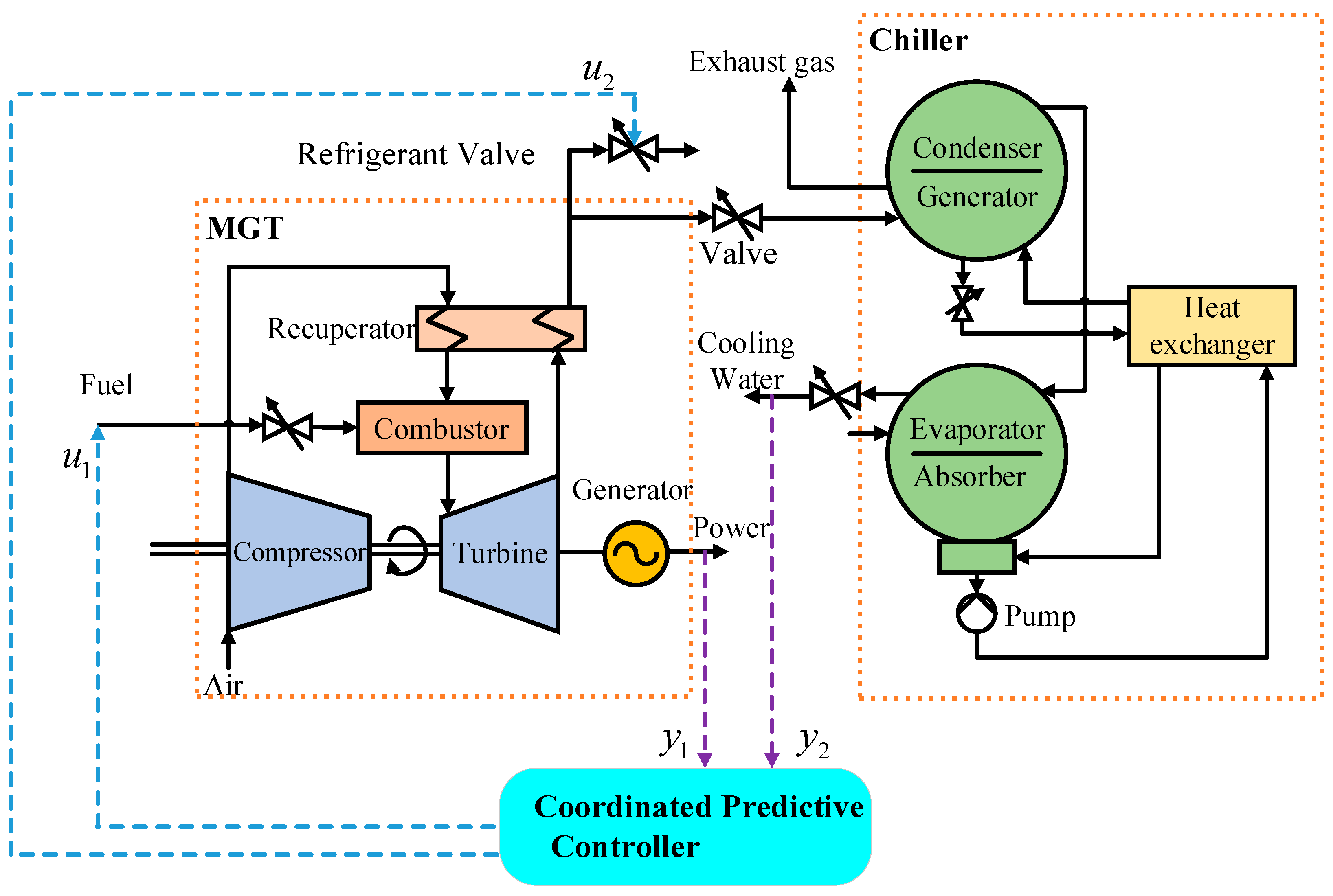
A MGT-CCP system, composed of an 80 kW full heat-regenerated-cycle MGT and a 75 kW lithium bromide single effect absorption chiller, is considered in this paper. The MGT-CCP system schematic diagram is shown in
Figure 1. Fuel is supplied to the MGT to generate the required electric power, while the waste heat emitted from MGT is recycled to drive the refrigeration system to produce chilled water. The MGT-CCP system can generate electricity and chilled water for the power and cooling load requirements at the same time.
The study on control strategy is based on a MGT-CCP emulator, which is built on the MATLAB R2016b environment and consists of dozens of major lumped-parameter modules and other functional components. Built on three conservation laws and thermal property equations, the emulator shows quite close dynamic characteristics to the primary MGT-CCP system. The detailed process of modeling is referenced in [
25] and the main design data of the MGT-CCP system is given in
Appendix A.
It is worth noting that the exhaust temperature of the fully heat-regenerated MGT is 277 °C, which is much lower than the non-heat-regenerated MGT of about 615 °C. Considering the limitation of heat exchange efficiency and avoiding the corrosion of low temperature flue gas in the pipeline, the exhaust temperature of the final flue gas of MGT-CCP is designed to be 170 °C. Therefore, the thermal power generated by the chiller is about 75 kW. A ratio close to 1.0 between thermal power and electrical power means that power generation efficiency is more preferentially improved in such an all-heat regeneration MGT-CCP system.
In order to help designing the controller, the MGT-CCP system can be regarded as a double-input-and-double-output dynamic system. The manipulate variables are fuel and refrigerant valve opening . The output variables are power output and chilled water temperature .
Table 1 is the typical operating points of the MGT-CCP system, where
is power output, and
is chilled water temperature.
Remark 1: The chilled water temperature, rather than the cooling power, is chosen as the operating point for the MGT-CCP system. In the MGT-CCP system, the cooling power is proportional to the product of the temperature difference and the chilled water flow. Since the flow rate of chilled water is assumed to be constant, from a control point of view, the chilled water temperature can represent the cooling power. Although the water flow is disturbed during operation, the chilled temperature can indicate the required cooling power generation. In addition, temperature has the advantage that it can be measured directly.
Based on the simulator, the following analysis will use two methods to expose several control issues for the MGT-CCP system. First, an open-loop step response test is performed to show the change in dynamic behavior. Second, the gap metric method is used to determine the degree of nonlinearity of the system by measuring the dynamic difference between models linearized at different operating points; thus, providing a quantitative description of the nonlinearity distribution of the MGT-CCP process.
2.1. Dynamic Analysis
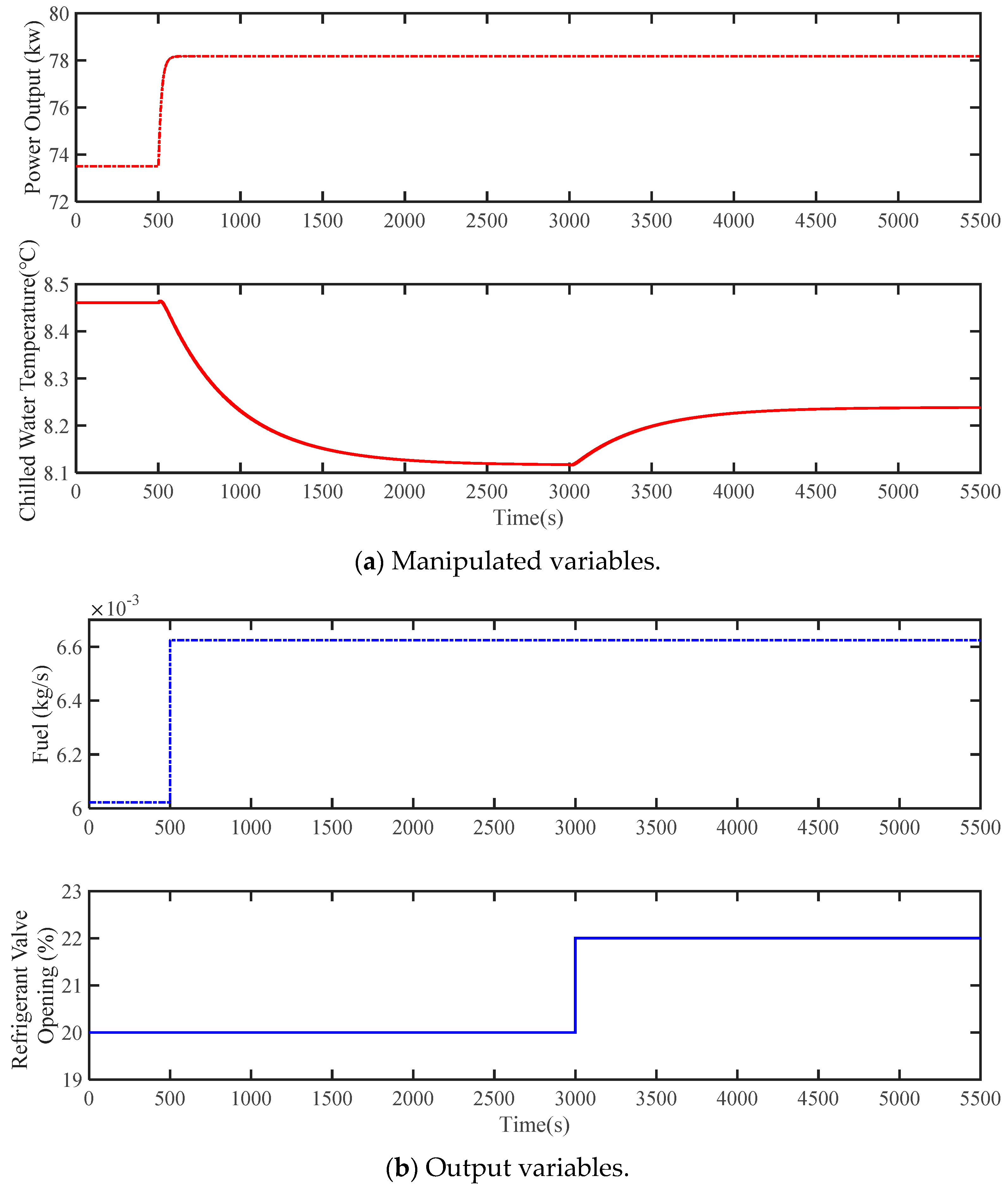
Suppose the system is running at operating point #3 in
Table 1. At 500 s and 3000 s, a +10% step signal of the corresponding steady-state value is added to the fuel and the refrigerant valve opening, respectively. The response of the plant is shown in
Figure 2.
Figure 2 shows that the power output responds very quickly to the fuel step command because it has very fast dynamic response characteristics. In addition,
Figure 2 shows that as the fuel step increases, the chilled water temperature slowly decreases to a constant value. The reason for the slow response of the chilled water is caused by exhaust gas transport and heat transfer in the chiller. It is easy to understand that the more fuel entering the MGT and the more exhaust gas entering the chiller, the greater the power of the chiller. Therefore, when the fuel is increased, the chilled water temperature is lowered. At 3000 s, the refrigerant valve opening increases, resulting in a decrease in exhaust gas entering the chiller, thus causing a decrease in chilled water temperature. As seen from
Figure 1, the chiller is located behind the MGT, so the power output does not change when the refrigerant valve opening changes.
The large inertia of the chilled water temperature is due to the exhaust gas transmission and thermal transferring process in the chiller. First the lithium bromide solution is heated in the generator by the exhaust gas which is a desorption process of solution. The vapour out of the solution condenses into the refrigerant water by releasing its heat to the cooling water in the condenser. The refrigerant water flows through the throttle valve and then evaporates in the evaporator and absorbs heat from the chilled water and cools it down. All these processes in the flowchart of the chiller, shown in
Figure 1, contributes to a large inertial from the fuel change to the variation of chilled water temperature. Another input the refrigerant valve is a bypass valve for the exhaust gas to the chiller, thus it influences the chilled water temperature in the same direction slowly.
To conclude, the power output is affected only by fuel, so for the safety and flexibility of MGT-CCP, a separate controller is designed for the control loop of power output. The chilled water temperature is affected by both fuel and refrigerant valve opening. There is a strong coupling between the variables. Therefore, when designing the control loop of the chilled water temperature , it is necessary to coordinate the control with the control loop of the power output . In addition, the chilled water temperature response has a large inertia, so it is necessary to study advanced control methods to replace the traditional PID control.
2.2. Nonlinear Analysis via Gap-Metric
Vinnicombe gap (V-gap) metric has been successfully applied to multi-model modeling and control of power plant boilers-turbine [
26] and spacecraft attitude control [
27], providing an appropriate partition of the operating region and the selection of local models, making it possible to use a minimum number of linear models to approximate the nonlinear behavior of the system.
The value of V-gap is a measure of the difference between two linear models. Suppose
and
are the transfer functions of linear models at any two operating points of the MGT-CCP system. The V-gap between
and
can be computed by:
where
and
are the elements of the normalized right coprime factorization of
and
as:
and
, and
is a matrix parameter which has finite H-infinity norm. The detailed process of gap calculation is referenced in [
28], which has been programmed as a
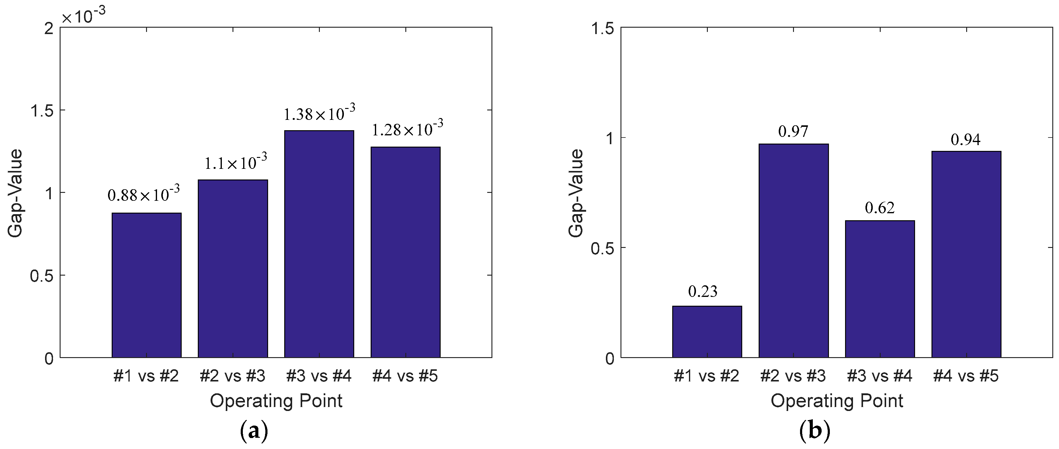
function in the MATLAB toolbox. The value of V-gap is between 0 and 1. The greater the value of V-gap, the greater the difference between the two linear models, that is, the stronger the nonlinearity of the region.
This section proposes the use of V-gap to quantitatively analyze the nonlinearity distribution of the MGT-CCP process over the operating range (power output: 65.18 kW–80 kW; chilled water temperature: 8 °C–9.1 °C).
A local linear model is first developed for a specific operating point for gap metric calculations. At each operating point, a random identification signal with a steady-state value of ±2% for 3000 s is applied to the fuel and the refrigerant valve opening path, respectively, to generate a corresponding output signals. A linear model for each operating point in
Table 1 is built using the System Identification Toolbox in MATLAB based on the resulting input-output data. The gap metric between adjacent linear models is then calculated to indicate the level of non-linearity along the corresponding region as shown in
Figure 3.
Figure 3a is a nonlinearity distribution of the MGT-CCP process under varying fuel. The results show that the gaps between adjacent operating points are small and uniform, implying that one linear model is sufficient for operating points #1 through #5. Therefore, in
Section 4, a linear controller is designed for the control loop of the power output.
Figure 3b shows the nonlinearity distribution of the MGT-CCP process under varying refrigerant valve opening. The gaps between the operating points #2 and #3 and #4 and #5 show extreme nonlinearity, and the gap between the operating points #3 and #4 also shows nonlinearity. The gap between the operating points #1 and #2 shows the least nonlinearity. The physical processes of the chiller include desorption and absorption of the lithium bromide solution, phase change of the liquid, and various heat-transferring processes. Its physical structure is complex, which leads to its inevitable nonlinear dynamics. Therefore, in
Section 4, a nonlinear controller is designed for the control loop of the cold-water temperature.
3. Identification of Multivariable Hammerstein Model
Predictive control offers its own distinctive features for dealing with coupled variables in process control, such as large inertia, input constraints, etc. It can also handle the predictive control of nonlinear plant well with a nonlinear predictive model. Therefore, predictive control is an appropriate solution for the combined cooling and power load-following control of MGT-CCP.
In the design framework of the predictive controller, designing a prediction model takes the lead. The Hammerstein model consists of a static memoryless nonlinear element and a dynamic linear model [
29,
30]. It has the advantages of small computing load, strong nonlinearity-approximating ability, and favorable controller design. Since the nonlinearity of the cooling system is very strong, the Hammerstein model is taken to be the prediction model for generalized predictive controller (GPC) whose algorithm matches well with the prediction model. An effective Hammerstein model identification method for SISO system has been proposed in [
24], which we extend to multi-input-single-output (MISO) systems for modeling the MGT-CCP.
Assuming that a system with
-input and single-output can be described by the following Hammerstein model:
where
and
are polynomials in the shift operator
with:
The following assumptions are made:
Assumption 1. Suppose the order of polynomial and are equal to . It is assumed that and are both known, or can be determined by trial and error.
Assumption 2. The first coefficient of the function
equals 1; i.e.,
[
24].
Assumption 3. The order of the function
is
. Suppose
is even, then there is at least one real root of (20). In this way, one is guaranteed that a value of
can be found [
30].
Then (2) can be rewritten as follows:
where
represents the element of the
-th column of
.
Define the following vectors:
Then (3) can be rewritten into the following form:
and the recursive least squares method is used to identify parameters
:
where
represents the current moment,
represents the parameter estimation at the previous moment.
After obtaining the estimated value of the parameter , the parameter can be obtained directly from , but the parameter also needs to be separated from the parameter . Without loss of generality, let’s assume that , then can be obtained directly from the first to lines of .
After obtaining the parameter
, the remaining parameter
of the nonlinear function is obtained by:
where
represents the
-th row element of
.
In summary, the linear and nonlinear coefficients of the Hammerstein model (2) of the MISO system can be obtained through Equations (6) and (7), and the obtained Hammerstein model of the cooling system of the MGT-CCP will be shown and verified in
Section 5.
4. Coordinated Predictive Controller Design
In this section, first we introduce the GPC algorithm, then propose the Hammerstein-GPC algorithm, and finally design the coordinated predictive control system for the MGT-CCP system.
4.1. Generalized Predictive Control
Consider the following controlled auto-regressive integrated moving average (CARIMA) model:
where
represents the discrete time,
represents the post-shift operator,
represents the difference operator,
represents noise, and
and
are polynomials in the shift operator
with
,
.
Ignoring the noise term
, the Equation (8) can be written as follows:
which then can be expressed as
Consider the following Diophantine equation:
where
and
are polynomials in the shift operator
with
,
.
Combining the Equations (8) and (11), through some mathematical transformations, we can get the system output prediction value
at time
:
In GPC algorithm, the optimization performance indicator at time
takes the following form:
where
represents prediction horizon,
represents control horizon,
represents the error weight coefficient,
represents the control weight coefficient, and
represents the expected reference value of the system output.
Then (12) can be rewritten as follows:
where
.
According to (15) we can easily get the following formula:
where:
Because of the influence of model error and disturbance, the output prediction value of the system needs to be corrected by the actual output error on the basis of the output of the prediction model:
where
is the prediction error,
is the actual output of the object, and
is the predicted output of the object. According to (13) and (17), the following can be obtained:
where
,
represents the error weighting matrix,
represents the control weight matrix, and
represents the unit matrix.
The output variable of the GPC algorithm is obtained according to (18):
4.2. Hammerstein Model-Based Generalized Predictive Control
Consider the SISO Hammerstein system as follows:
where (20) is a static nonlinear element without memory, (21) is a dynamic linear model,
and
are the order of the linear model,
and
are the parameters of the linear model,
and
are input and output of the system, respectively, and
is the intermediate variable.
The system model given by (20) and (21) shows that the control input
affects the system output
through the intermediate variable
. Although the relationship between
and
is nonlinear, the relationship between
and
is linear. Therefore, the GPC algorithm is designed with the linear model (21) first, i.e., the desired intermediate variable
is calculated through the receding-horizon optimization of the GPC algorithm. Then the control action
is solved from nonlinear algebraic Equation (20). The structure of the Hammerstein-GPC controller is shown in
Figure 4. This control strategy makes full use of the special structure of the Hammerstein model and is actually a nonlinear separation strategy, which makes the whole solution simple.
4.3. Coordinated Predictive Controller Design for the MGT-CCP System
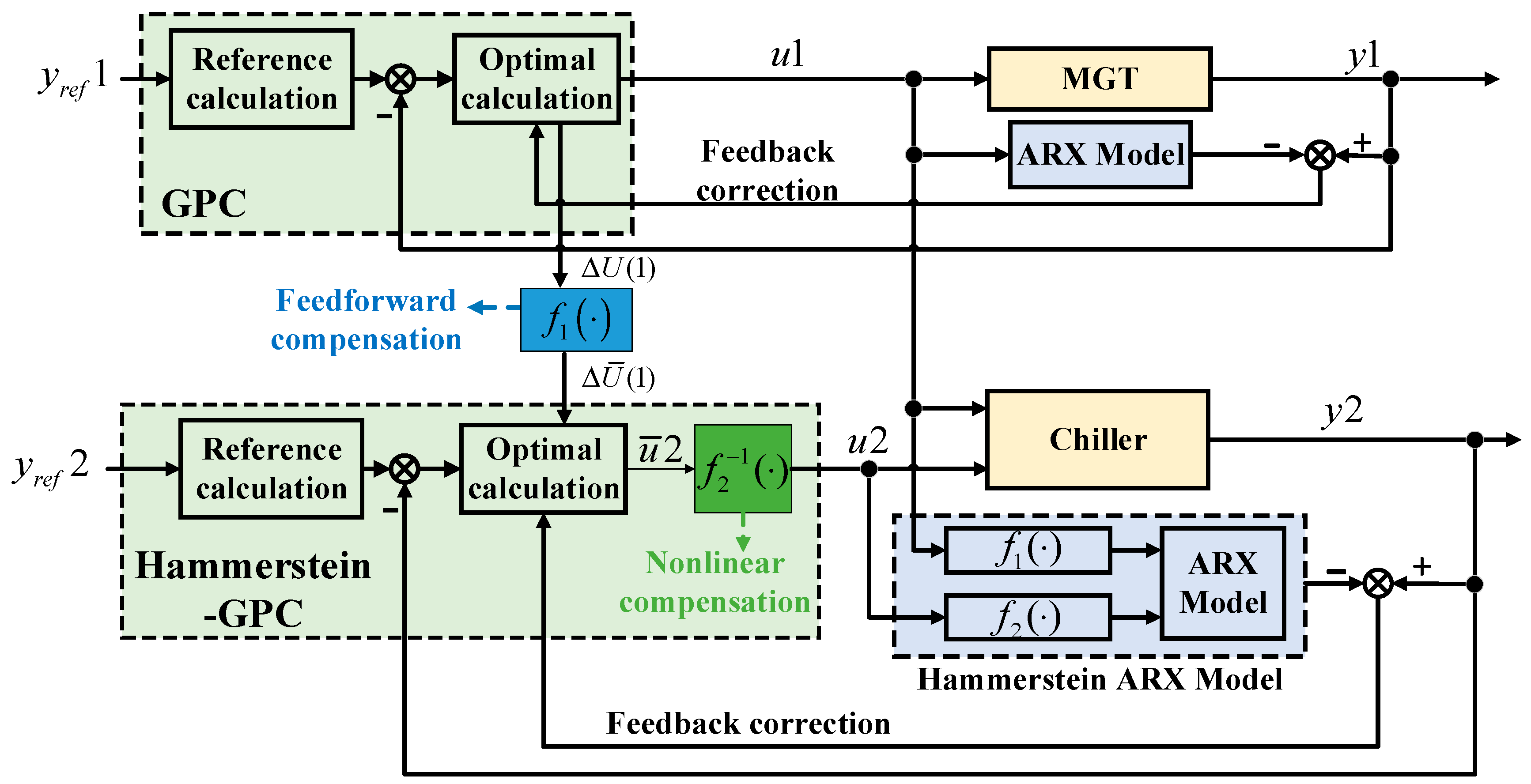
This section presents the coordinated predictive control strategy for the MGT-CCP system, as shown in
Figure 5.
Considering the physical characteristics of the MGT-CCP system, the MGT-CCP system was split into a power supply system and a cooling system. In view of the degree of nonlinearity of the two subsystems, the linear GPC is designed for the power generation system and the nonlinear Hammerstein-GPC is designed for the cooling system. The nonlinearity of the cooling system is effectively suppressed by nonlinear compensation, and the coupling between subsystems is effectively weakened by feedforward compensation. Besides, due to the inevitable modeling error, feedback correction is adopted in the proposed control strategy.
The main calculation process of the GPC-HGPC coordinated control algorithm is summarized as follows:
- (1)
At time , the calculation of the linear GPC controller is performed, and the optimal input increment sequence of the fuel amount is calculated, and the optimal control variable of the MGT system is further obtained;
- (2)
The intermediate control variable sequence is calculated by using the fuel quantity optimal input increment sequence and the nonlinear polynomial ;
- (3)
Adding the sequence
as feedforward information to Equation (15) gives an output prediction of chilled water temperature:
where
. Note that
is known at time
;
- (4)
Based on (22), using the linear GPC algorithm to calculate the intermediate control variable increment sequence , and then obtain ;
- (5)
Using the intermediate control variable and the inverse of the nonlinear polynomial to obtain the refrigerant valve opening ;
- (6)
Next sampling time, return to step (1), repeat steps (1) to (5).
Remark 2: For the sake of simplicity, the proposed method uses the control model obtained by offline identification. If the actual MGT-CCP system has large time-varying characteristics, the performance of the proposed control algorithm will be attenuated. But this problem can be overcome by adding online identification of the control model.
Remark 3: This algorithm can only eliminate the influence of external disturbance of the step type. For time-varying disturbances, adding on-line identification of the disturbance model to the proposed algorithm can improve control performance [
31].
5. Simulation Results
This section verifies the effectiveness of the multivariate Hammerstein model identification strategy and the coordinated predictive controller designed for the MGT-CCP system. First, the accuracy of the multivariate Hammerstein model was verified, and then the proposed coordinated predictive controller was tested and compared to the PI controller.
5.1. Verification of Identification Model
5.1.1. Power Generation System
The power generation system is affected only by the fuel, so it can be considered as a SISO system. According to the nonlinear analysis in
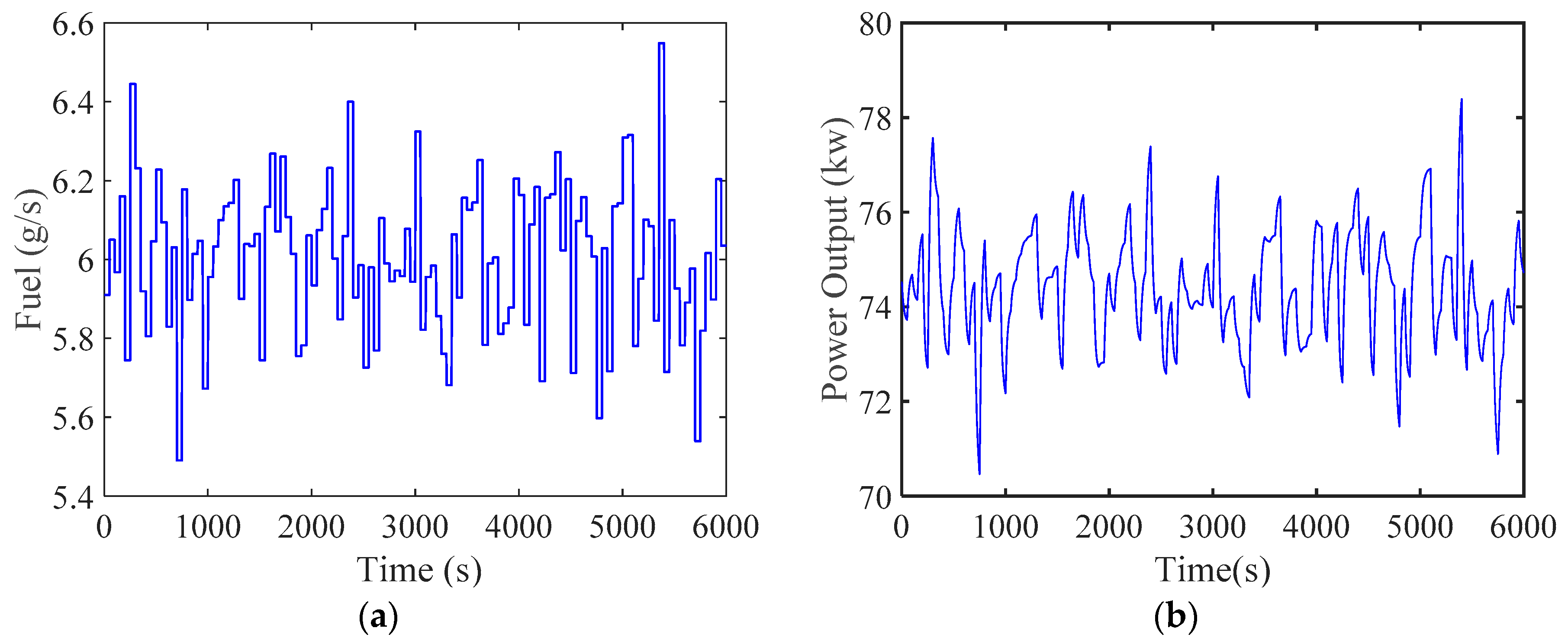
Section 2, the nonlinearity of the power generation system is weak, so the conventional recursive least squares method is used to identify the model of the power generation system. The input sequence shown in
Figure 6a is applied to the MGT-CCP system to obtain the output data shown in
Figure 6b. The model of the power generation system was identified using the first 3000 s of data. The identified input and output models are as follows:
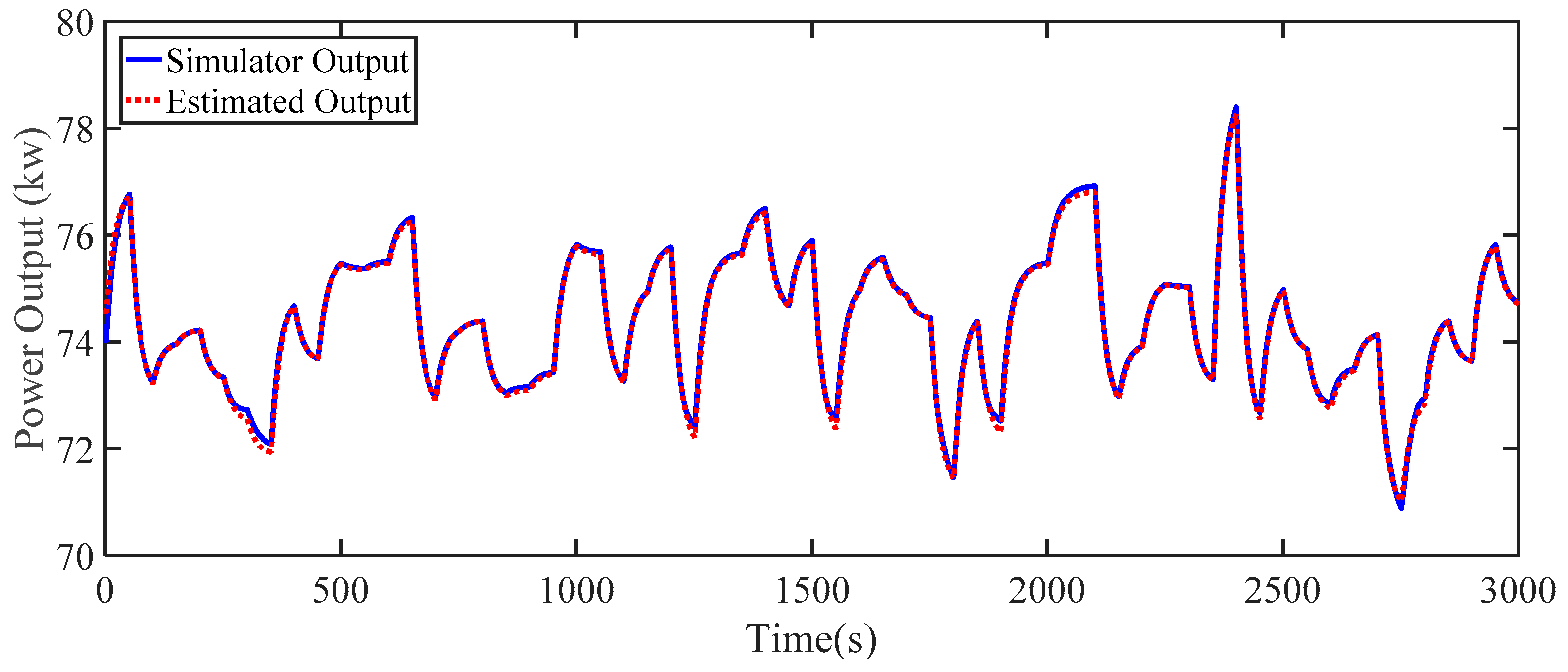
The accuracy of the identification model is verified using the last 3000 s of the data of
Figure 6. The verification results are shown in
Figure 7. It can be seen that the identified linear model has high accuracy, which also indicates that the nonlinearity of the power supply system is very weak, which is consistent with the nonlinear analysis results in the second section.
5.1.2. Cooling System
The cooling system is affected by both the fuel and the refrigerant valve opening, so the cooling system can be viewed as a two-input single-output system. According to the nonlinear analysis in
Section 2, the nonlinearity of the cooling system is very strong, so the Hammerstein model identification method proposed in
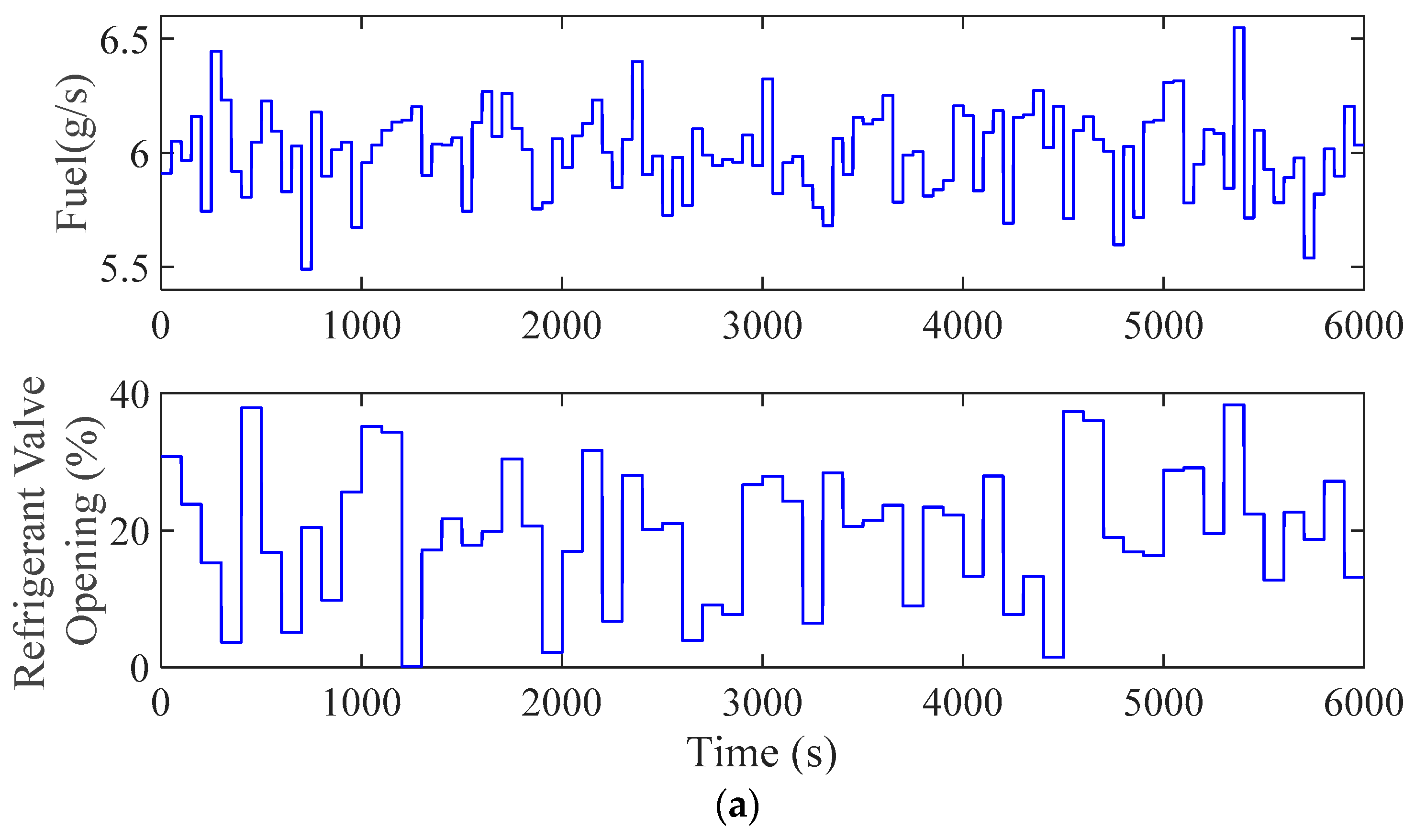
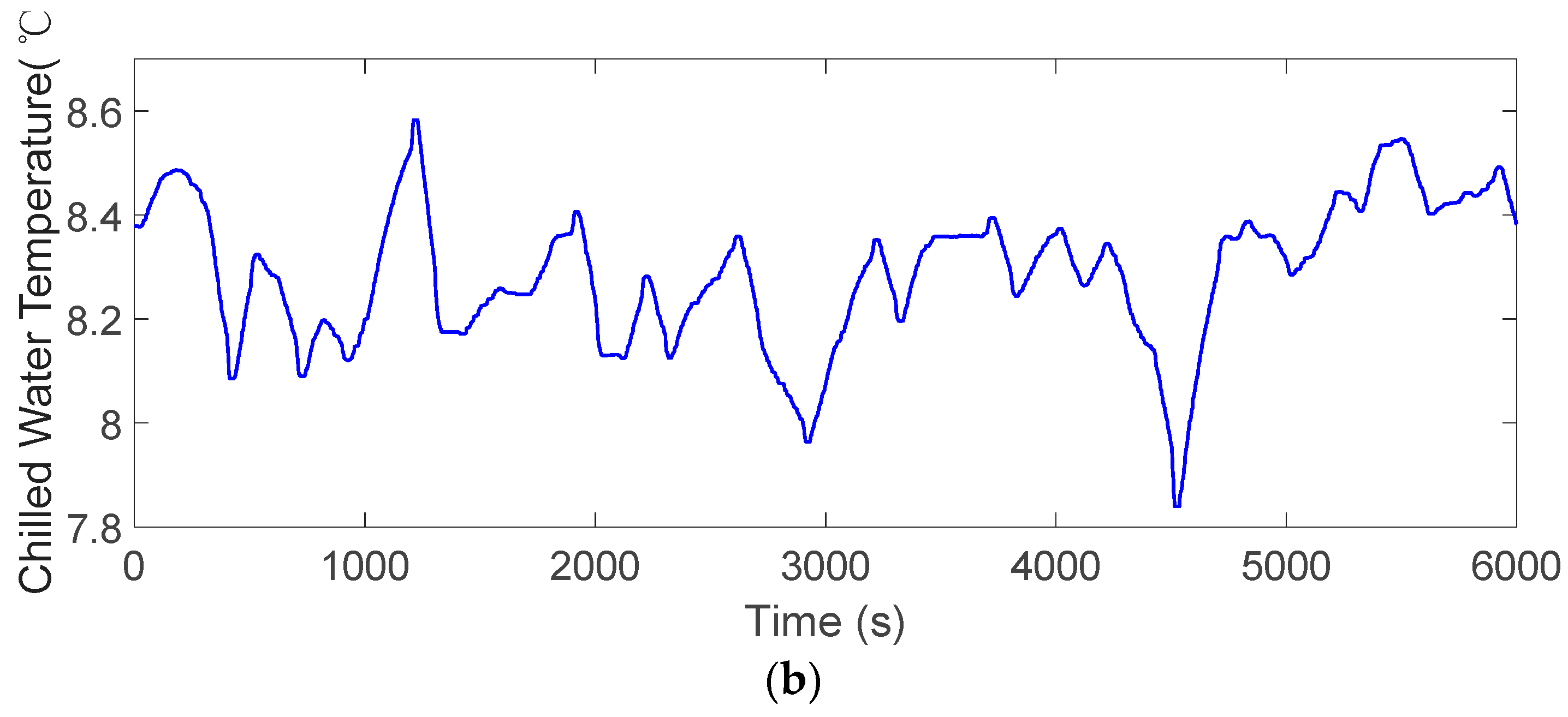
Section 3 is used to identify the model of the cooling system. The input sequence shown in
Figure 8a is applied to the MGT-CCP system to obtain the output data shown in
Figure 8b. The model of the power supply system was identified using the first 3000 s of data. The identified Hammerstein model is as follows:
where
.
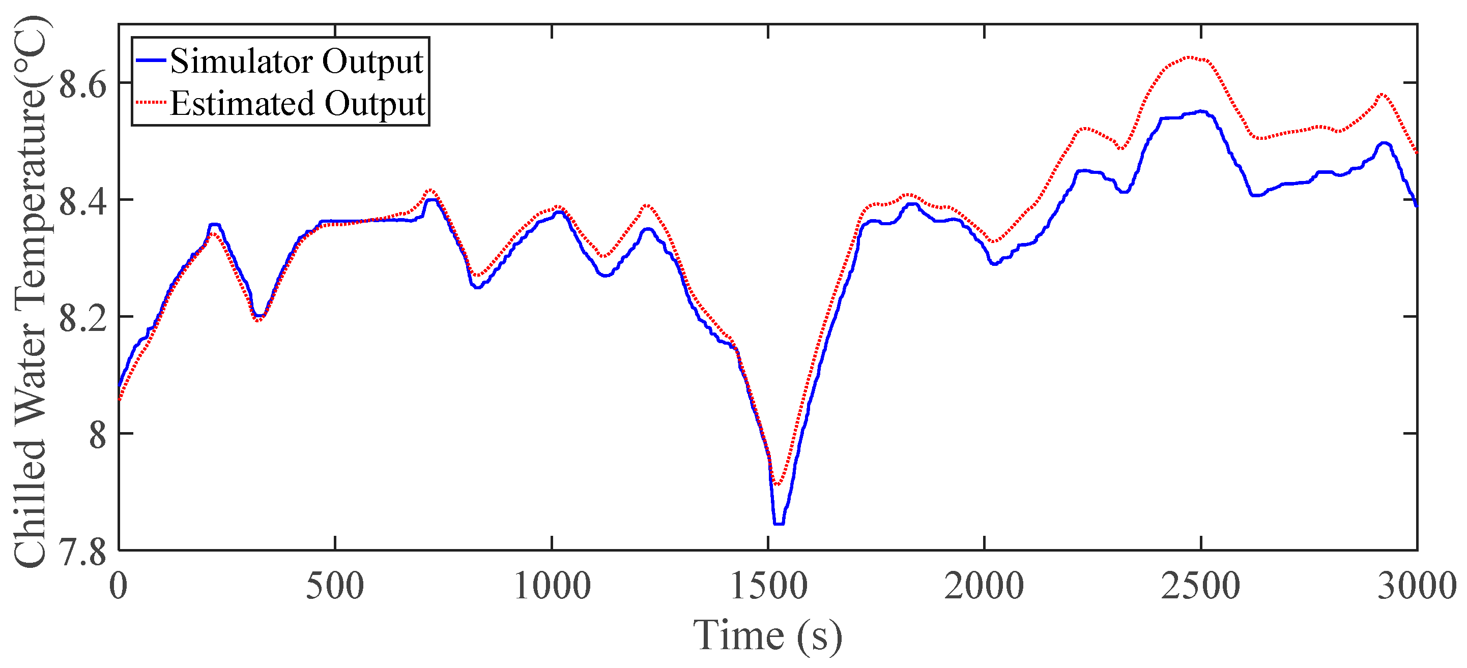
The accuracy of the identification model is verified using the last 3000 s of the data of
Figure 8. The verification results are shown in
Figure 9. It can be seen that the identified Hammerstein model has high accuracy and can reflect the changing trend of the system.
5.2. Testing of the Proposed Control Strategy
This section tests the proposed GPC-HGPC coordinated controller for the MGT-CCP system. The parameters of the proposed controller are set as follows: for linear GPC controllers, prediction horizon , control horizon , error weight coefficient , control weight coefficient ; for the Hammerstein-GPC controller, prediction horizon , control horizon , error weight coefficient , control weight coefficient .
The PID controller and MPC control are compared with the proposed controller. The parameters of the PID controller are as follows: for the power supply system, the proportional gain , the integral gain , the differential gain ; for the cooling system, the proportional gain , the integral gain , the differential gain . Note that the PID controller is optimally tuned using the Tuner function of the PID module provided by Simulink.
The parameters of the MPC controller are as follows: prediction horizon , control horizon , sampling time , control weight coefficient , control rate weight coefficient , output weight coefficient .
The control structure of the comparison methods is shown in
Figure 10.
In order to quantitatively compare the load tracking performance of different controllers, the integrated absolute error (IAE) is used in the following simulations. IAE is given by:
5.2.1. Case 1: Simultaneous Cooling and Power Load-Following Performance
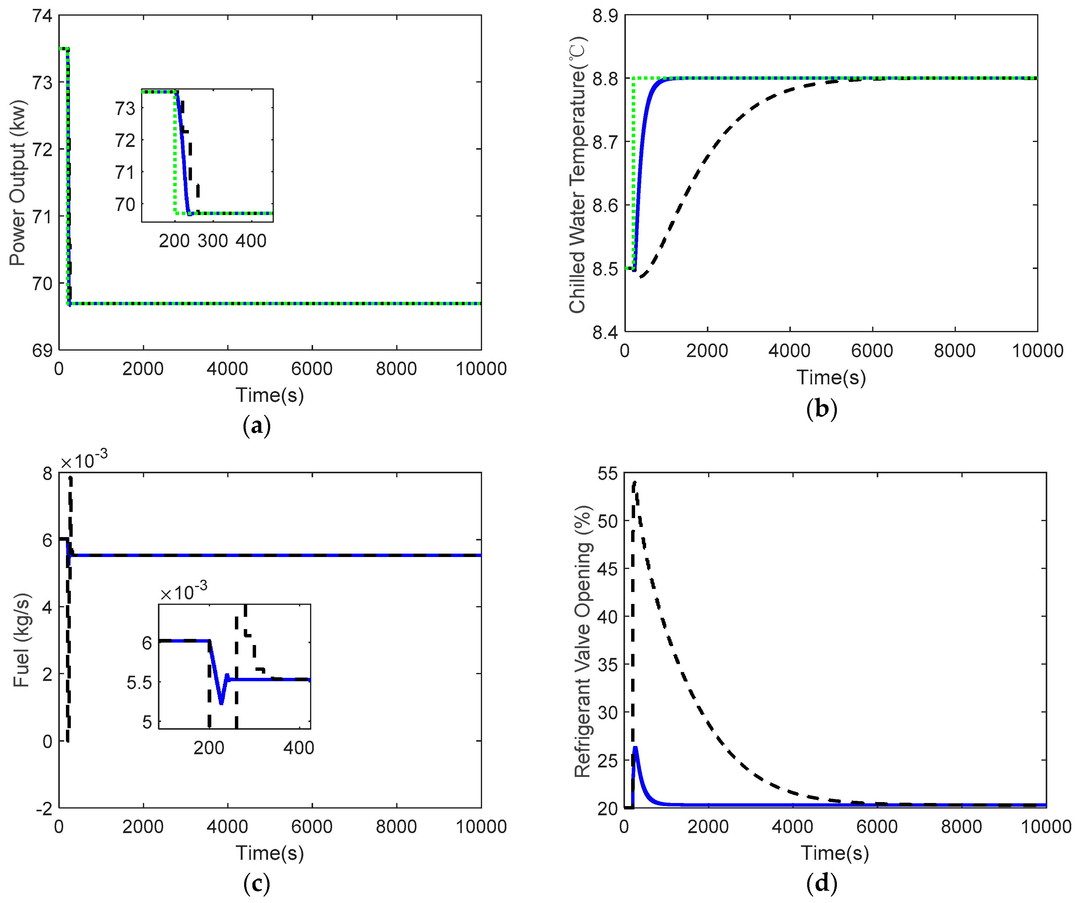
Case 1 was designed to test the simultaneous cooling and power load-following performance of controllers. First, compare the proposed method with conventional MPC. Assume that the MGT-CCP system is operating at point #3. At 200 s, the MGT-CCP system changes from the operating point #3 (
) to the operating point #4 (
). The simulation results are shown in
Figure 11 and
Table 2.
Both the proposed method and the conventional MPC can track the set points. But the proposed method is faster for load tracking. The power tracking performance under the IAE indicator increased by 7%, and the cold load tracking performance increased by 80%. The reason is that the proposed method uses coupling compensation and nonlinear compensation strategies.
Then we test the tracking performance of the controllers for a wide range of load changes. At 1500 s, the MGT-CCP system changes from the operating point #4 (
) to the operating point #5 (
), and then keeps running at the operating point #4, at 3000 s, the MGT-CCP system changes from operating point #5 to operating point #1 (
), and finally keeps running at operating point #1. The simulation results are shown in
Figure 12 and
Table 3. The simulation results show that the proposed method has smaller overshoot and faster tracking speed. The power tracking performance under the IAE indicator increased by 48%, and the cold load tracking performance increased by 20%.
5.2.2. Case 2: Performance of Unknown Input Disturbances Rejection
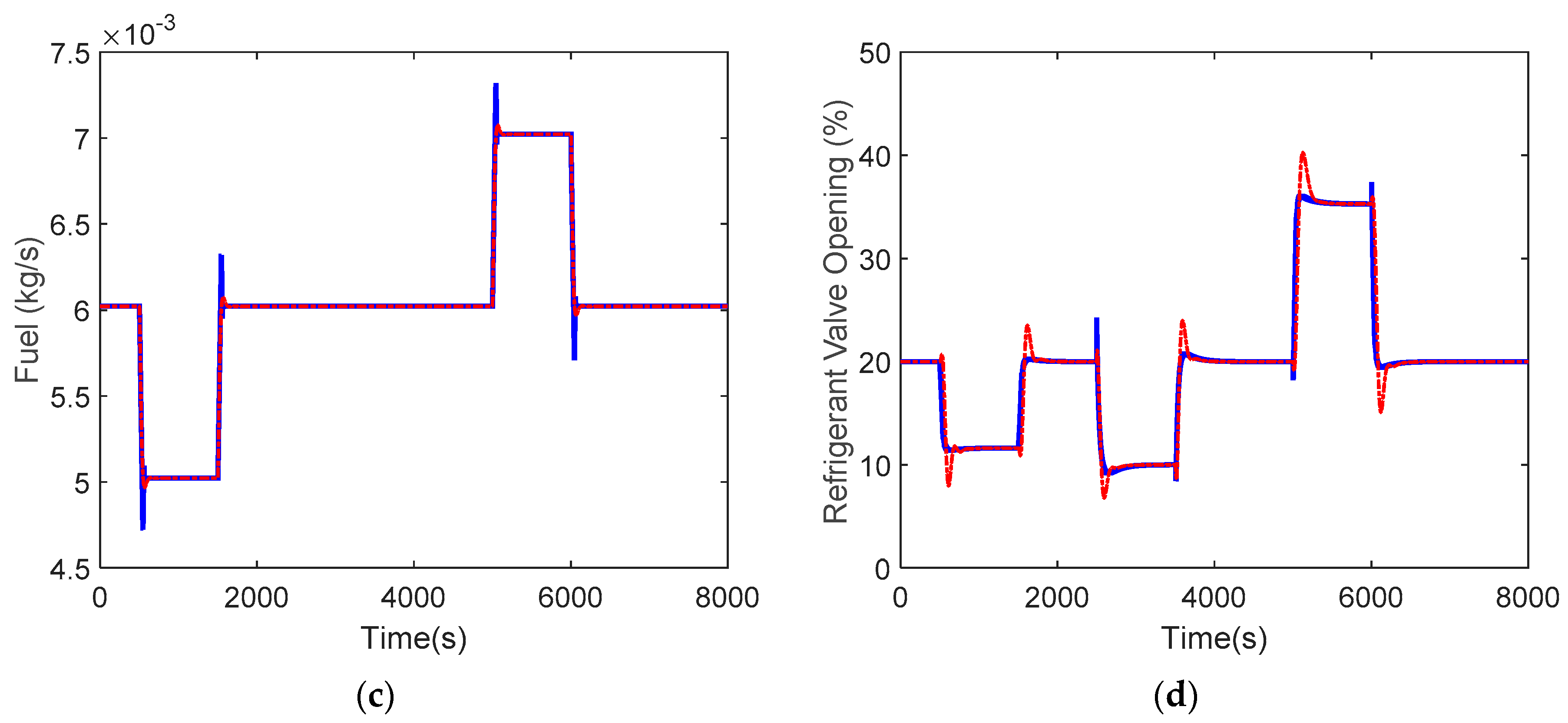
Case 2 is used to test the controller’s ability to suppress unknown input disturbances. Since the MGT-CCP system operates in a high temperature environment, the wear caused by the frequent operation of the valve will affect its stability. Therefore, the impact of input disturbances on the MGT-CCP system cannot be ignored.
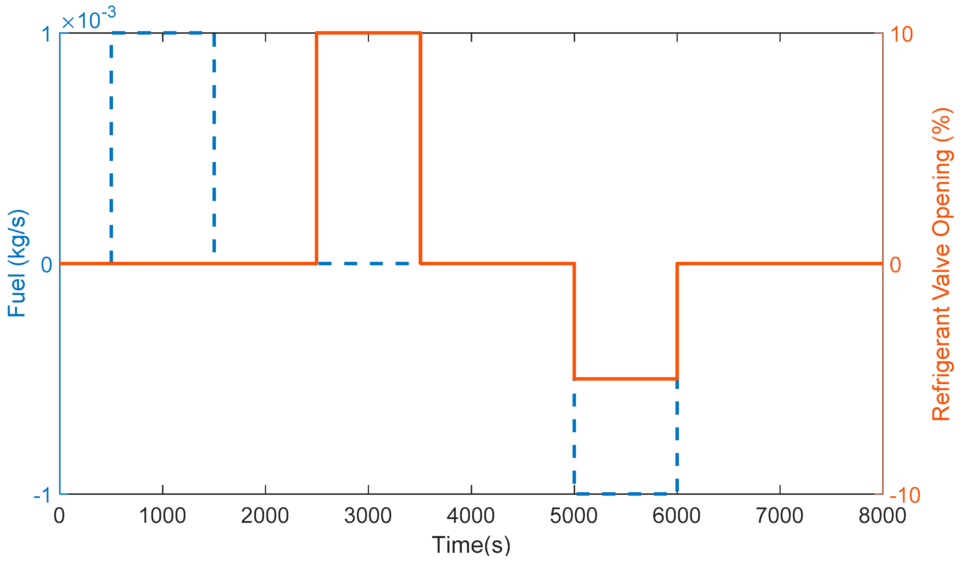
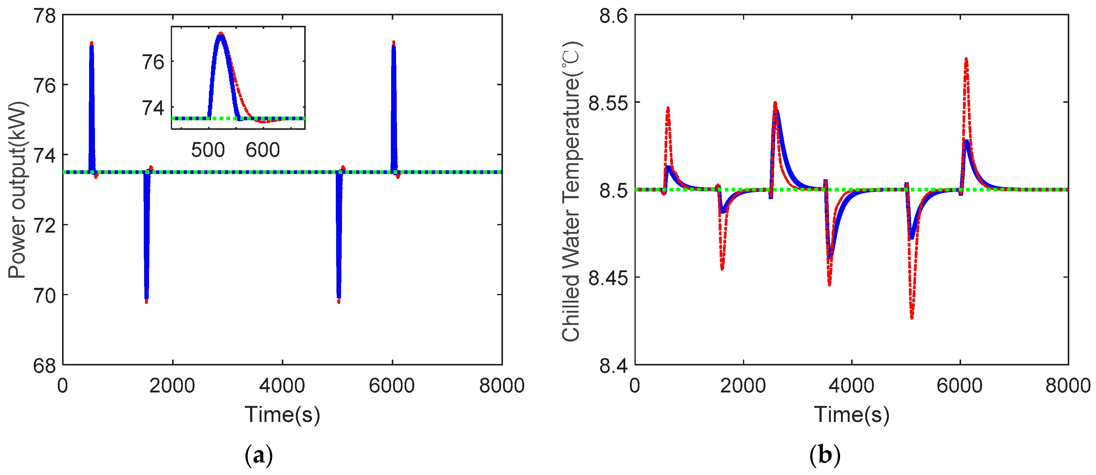
Assume that the MGT-CCP system is running at working point #3. The input side of the system is subject to unknown input disturbances as shown in
Figure 13, and the simulation results are shown in
Figure 14. The simulation results show that the controllers can eliminate the influence of unknown input disturbances, but the proposed method suppresses the disturbance faster and the deviation from the operating point is smaller.
5.2.3. Case 3: Tracking Performance on Time-Varying Power Load Demands
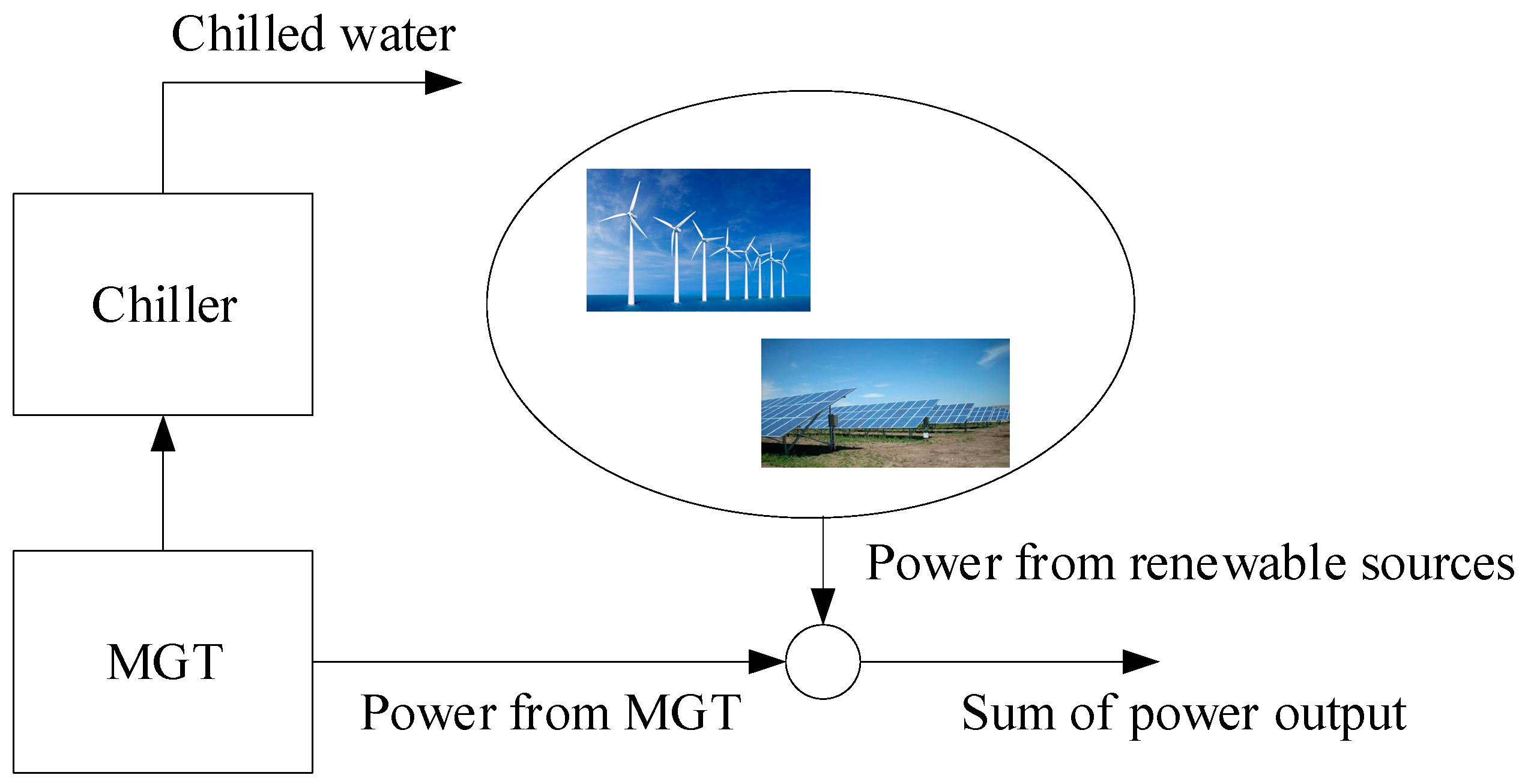
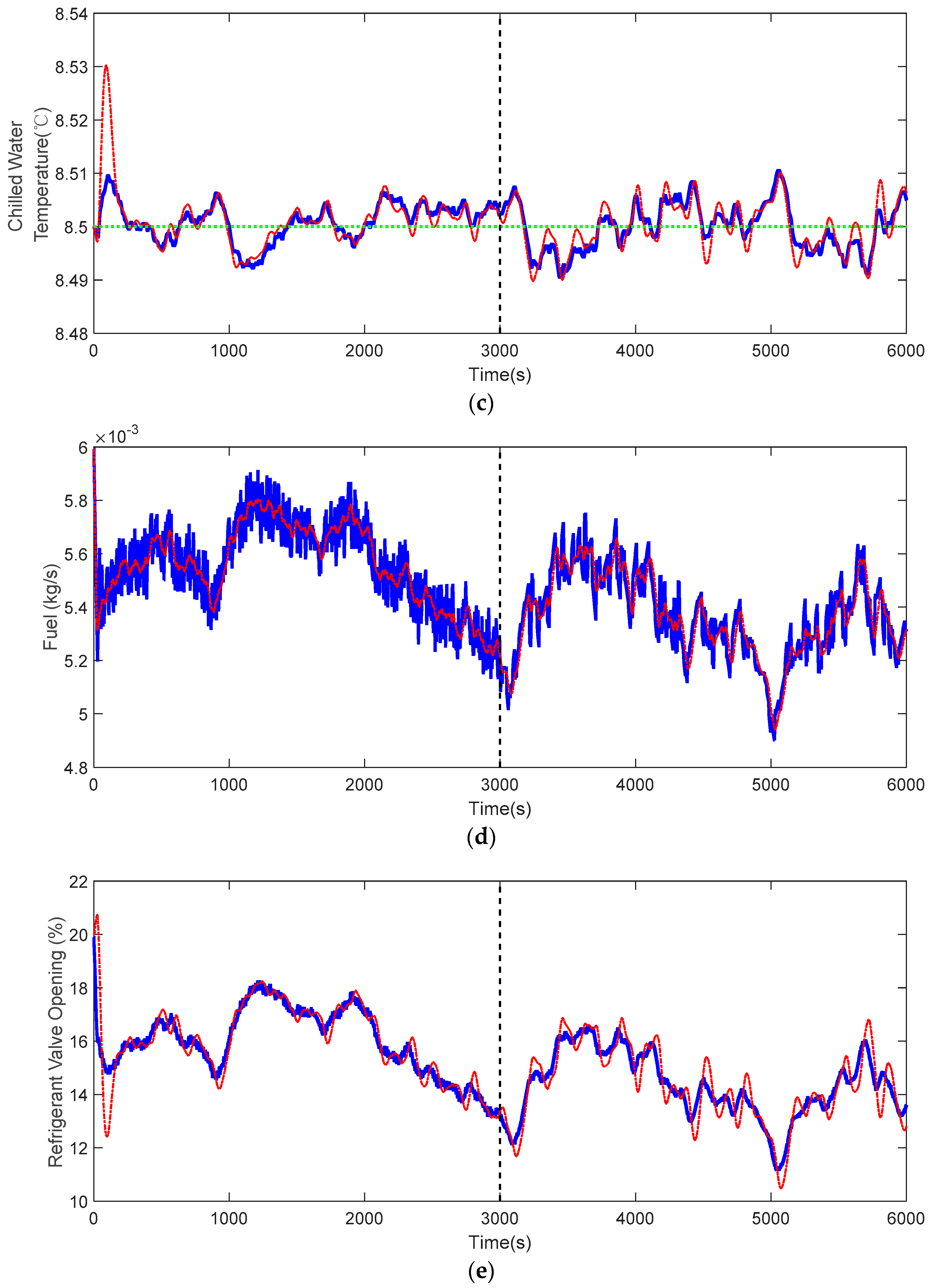
Renewable energy sources such as wind power and photovoltaic power have time-varying characteristics. When they are connected to a micro-grid with a MGT-CCP system, it is necessary to adjust the power output of gas turbine to maintain the stability of the micro-grid. Therefore, Case 3 tests the controller’s ability to track time-varying power load demands.
Figure 15 is a block diagram of the MGT-CCP system connected to renewable energy.
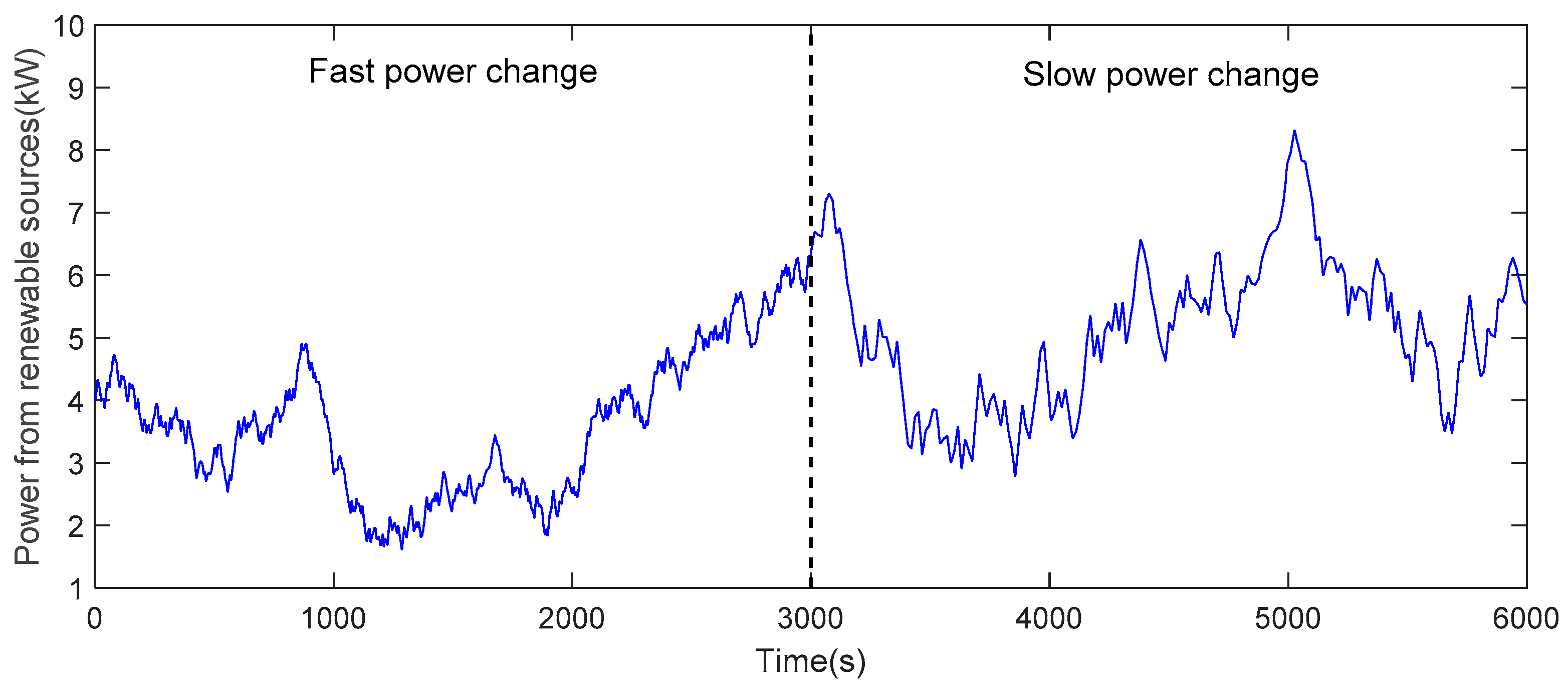
Assuming the MGT-CCP system is operating at operating point #3, the power required by the user is a fixed value and the power from the renewable sources is shown in
Figure 16. In order to verify the effectiveness of the proposed method in depth, in
Figure 16, the power changes rapidly in the first 3000 s, and the power changes slowly in the next 3000 s. The results are given in
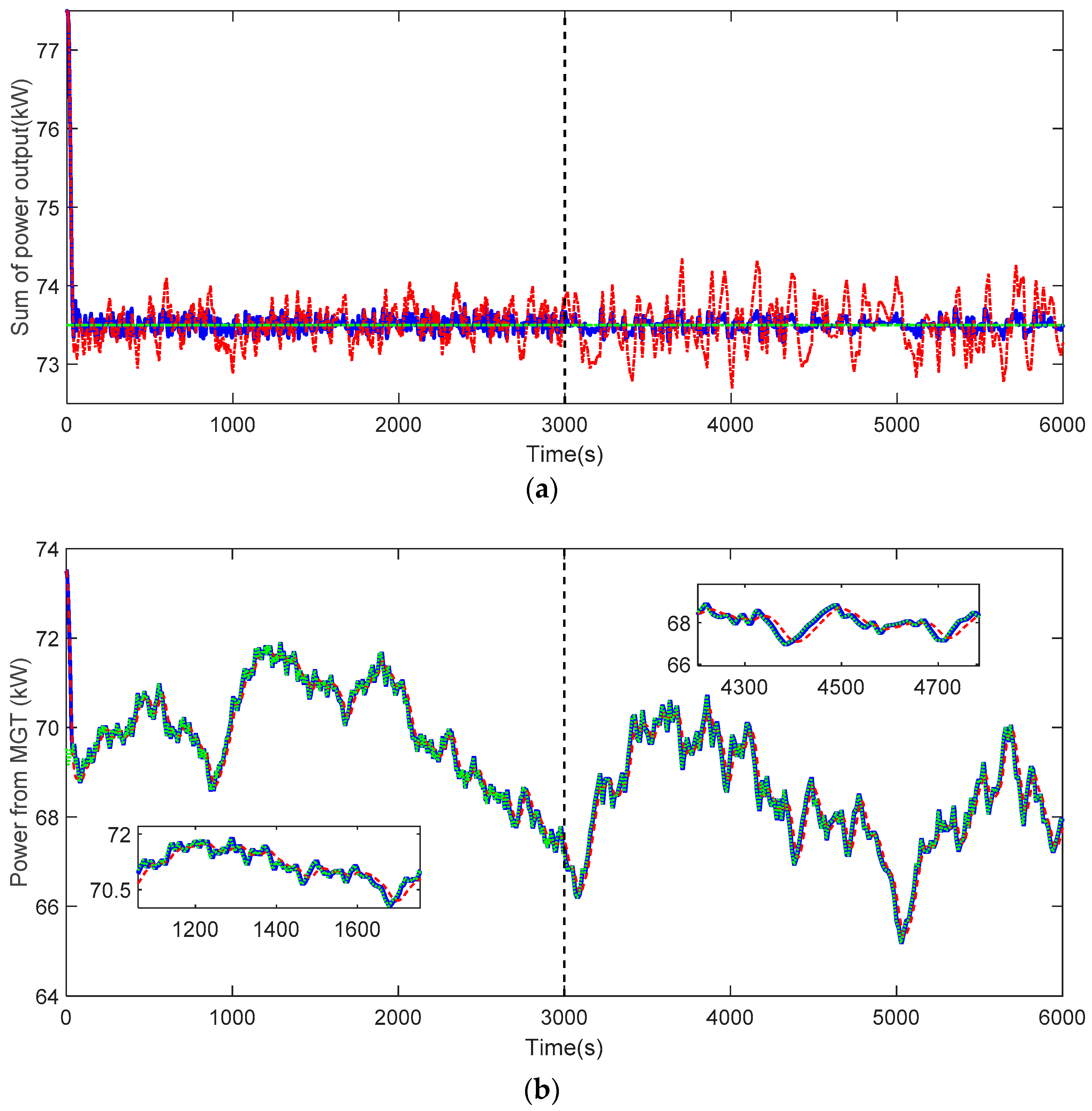
Figure 17 and
Table 4. The simulation results show that the proposed method can track the electric load command better, the tracking speed is faster and the dynamic deviation is smaller. In addition, because of the implementation of coordination, the cold-water temperature deviates from the set value by a smaller amount. The power tracking performance under the IAE indicator increased by 62%, and the cold load tracking performance increased by 9%.
6. Conclusions
In order to achieve a sustainable future with more renewable energy integrated into distributed energy systems, MGT-CCP systems must frequently change loads to achieve grid balance. This requires more flexibility in the operation of the MGT-CCP. To provide guidance for controller design, this paper first studies the dynamic behavior and nonlinearity distribution of the MGT-CCP process. The results show that the MGT speed is affected only by the fuel, and the nonlinearity of the power generation subsystem is extremely weak. However, the cold-water temperature is affected by both the fuel and the refrigerant valve opening, and the cooling subsystem is extremely nonlinear. Therefore, based on these results, a coordinated predictive control strategy is proposed to simultaneously improve cooling-and-power load-following capability. The simulation results show that compared with PID and MPC, the proposed control method not only can improve cooling and power load-following capability at the same time, but also has the best control effect when accessing with renewable energy. In the future, we will strive to consider economics into the controller design of the MGT-CCP system, which is also an important issue for implementation of predictive controls.
