Hybrid Adsorption-Compression Systems for Air Conditioning in Efficient Buildings: Design through Validated Dynamic Models

Abstract

Hybrid sorption-compression systems are gaining interest for heating/cooling/ refrigeration purposes in different applications, since they allow exploiting the benefits of both technologies and a better utilization of renewable sources. However, design of such components is still difficult, due to the intrinsic complexity of the systems and the lack of reliable models. In particular, the combination of adsorption-compression cascade unit has not been widely explored yet and there are no simulations or sizing tools reported in the literature. In this context, the present paper describes a model of a hybrid adsorption-compression system, realised in Modelica language using the commercial software Dymola. The models of the main components of the sorption and vapour compression unit are described in details and their validation presented. In addition, the integrated model is used for proving the feasibility of the system under dynamic realistic conditions and an example of the technical sizing that the model is able to accomplish is given.

1. Introduction

The building energy consumption across European Union accounts for about 40% of the overall primary energy consumption and, in this sector, the share of heating and cooling demand (also comprising domestic hot water) is about 55% [1]. For this reason, several national and international regulations have been issued to promote the energy efficiency in buildings, deriving from the Energy Performance of Buildings Directive (EPBD) issued by the EU [1]. Different approaches can be followed to increase the energy efficiency, which can be generally distinguished between passive and active methodologies. Among the passive ones, improvement of building insulation is considered as the most effective solution to meet the regulatory requirements [2]. Concerning the active methodologies, the main route is to improve the heating and cooling systems, by enhancing the efficiency of the heating and cooling devices [3], implementing smart control strategies [4,5,6] and integrating innovative solutions at system level [7,8]. In this context, one of the main focus is on increasing the share of renewables in the heating and cooling sector. Indeed, as already reported [9], the renewable heating and cooling sector is considered as a “sleeping giant” that, if properly promoted, could further support the diffusion of renewable sources especially in the residential and commercial sector. The heat pump technology is by definition able to exploit renewables, e.g., directly from ambient air [10] or from geothermal heat sources [11]. Nevertheless, the share of renewables guaranteed by standard heat pumps is limited, since they are usually driven by electrical energy. For this reason, in the last years, the exploitation of thermally-driven systems, able to make use of solar thermal energy as driving renewable source, was proposed, mainly for cooling applications, thus developing the so-called solar cooling technology [12]. The concept looks quite attractive, since it allows synchronizing the peak of solar radiation with the peak of cooling demand year-round. Some detailed reviews on this topic can be found elsewhere [13,14,15]. Nevertheless, some issues are still open to make it more attractive also for a future widespread diffusion on the market. One of the main critical tasks is represented by the needs of installing backup appliances (e.g., gas boiler, vapour compression chiller), to cover the periods during which solar energy is not available to drive the system. In order to overcome this issue, recently, integrated hybrid adsorption/ compression chiller solution was proposed in the literature [16]. This integration makes the operation more flexible, since the system can be efficiently driven by solar energy, when available, reducing the electric consumption to drive the vapour compression chiller, while can be directly switched to the standard chiller operation, when no thermal energy is provided by the solar thermal collectors. In this way, the overall solar fraction is maximized, guarantying the continuous operation of the system.

Despite the interesting approach, there is still a lack of dynamic models, which can be exploited to properly design and optimize the operation of this innovative hybrid solution. In particular, to the best of the authors knowledge, no models are available in the literature on the adsorption/compression hybrid technology. For this reason, in order to develop a consistent and reliable model, a careful analysis of existing models for adsorption and vapour compression machine components was performed. Generally, the models of components and energy systems can be distinguished as [17]:

• thermophysical models, making use of the constitutive equations of the system, that can be solved through a numerical or iterative approach;
• black box models, that are based on a completely empirical approach;
• grey box models, combining a semi-empirical approach with the physical models for one or more components.

A further distinction can be made according to the treatment of model variables with time, thus dividing the models into static, quasi-static and dynamic models. In the simulation of a wide variety of components it is common to use a black-box approach, using experimental data or performance data provided by suppliers to model complex energy systems with a low computational effort. Common simulation environments used are TRNSYS, Energy Plus and IDA-ICE, that were applied to a wide variety of systems, such as biomass-fed systems [18], fuel cells [19,20], solar systems with different types of heat pumps and chillers [21,22,23,24,25], fossil fuels and renewables-based cogenerators [26,27]. However, such a methodology can be too simplistic, especially when dealing with innovative components, whose response to a wide variety of external conditions is not yet known or fully characterised. As a result, some models were built integrating detailed physical equations and semi-empirical or lumped parameters models, i.e., by co-simulation in MATLAB-SIMULINK and TRNSYS environments [28,29,30]. The main drawback of such combined models is the low robustness and high computational effort, since two simulations engines running at the same time are needed. To overcome such issues, a tool often used to simulate complex multi-domain systems is the Modelica language, thanks to its low computational demand and a vast number of libraries including components for several energy systems, comprising heat pumps and chillers for commercial and residential applications [31,32,33,34,35].

A list of relevant and recent models for the components examined in the present study, i.e., an adsorption module for cold-water production and a vapour compression heat pumps is presented in

Table 1. Models of adsorption components and vapour compression heat pumps published in literature.

Reference	Components/Systems Modelled	Type of Model	Simulation Tool	Validation
[37]	Adsorption chiller	Grey-box (coupled heat and mass transfer model of the adsorber and lumped parameters model for the other components)	COMSOL/MATLAB	Yes
[38,39]	Adsorber, Adsorption chiller	Physical dynamic	Modelica	Yes
[34]	Adsorption chiller	Physical dynamic	Modelica	Yes
[40]	Adsorption material	Physical dynamic	COMSOL	Yes
[41]	Adsorption reactor	Physical dynamic	FEMLAB	No
[42]	System for adsorption refrigeration-desalination	Physical dynamic	Simulink	No
[43]	Coated adsorber	Physical–governing equations simplified to an ODE system	Not specified	Yes, with a numerical model of a 2-bed chiller
[21,44,45,46,47]	Adsorption chiller	Black box	TRNSYS	Models based on experimental data or datasheets
[48]	Adsorption-sensible storage	Grey box	TRNSYS/MATLAB	No
[49]	Air-water heat pump with R410a	Physical steady-state and dynamic	Modelica	Yes
[50]	Air-air heat pump with R134a	Physical dynamic	Modelica	Yes
[32]	CO2 heat pump	Physical dynamic	Modelica	No
[31]	Ground-source heat pump	Physical dynamic	Modelica	Yes
[35]	Variable speed heat pump	Grey box	Modelica/Dymola	Yes
[51]	Air-water heat pump	Grey box	MATLAB/Simulink	No
[52]	Water-water and air-water heat pumps	Exergy modelling	-	Yes
[24,44]	Air-water heat pumps	Black box	TRNSYS	No
[25,53]	Air-water heat pumps	Black box	IDA-ICE	No

.

Regarding hybrid sorption-compression systems, instead, only a few studies can be found in literature, as detailed in [16] and most of them refer to liquid absorption-vapour compression systems. Moreover, the vast majority of proposed models are based on steady-state thermodynamic evaluations [36], thus disregarding the discontinuous operation typical of adsorption systems.

In this context, the main aim of the paper is to develop the first simulation model able to dynamically represent the operation of a hybrid cascading adsorption/compression chiller. The model is based on a detailed description of each component, validated through experimental data published in the literature. It is implemented in Modelica/Dymola, to easily integrate the different sub-models. These were validated against experimental data for the adsorber and a complete performance map, for the compression chiller. In addition, the operation under realistic conditions was evaluated. To this aim, the cooling demand of a building in Agltanzia (Cyprus) was used. Indeed, the proposed hybrid system will be manufactured and tested within the H2020 HYBUILD project [34]. Indeed, the complete simulation tool was then used to perform a sensitivity analysis to provide possible hints for the optimization of the hybrid chiller design towards its real application.

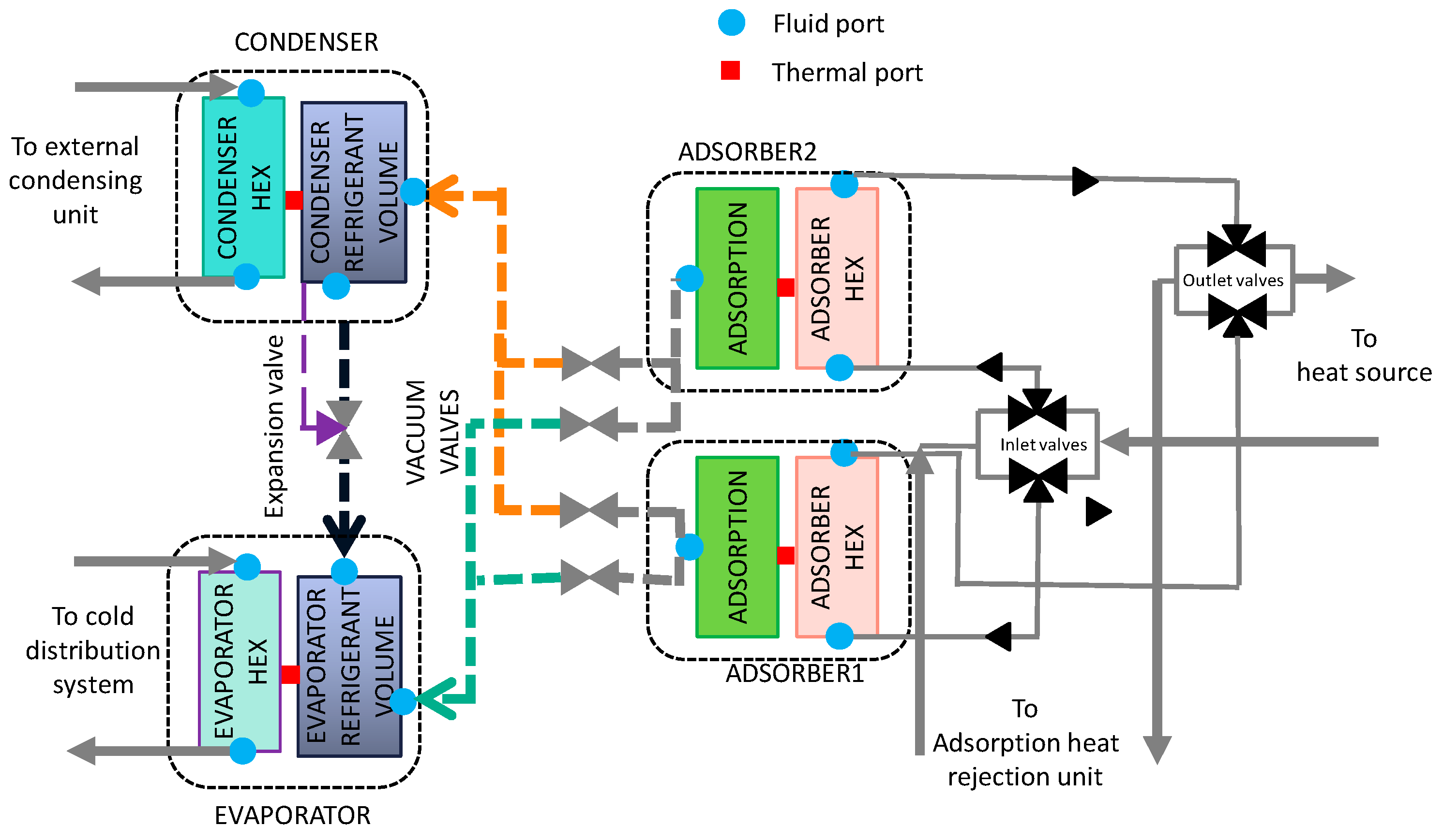
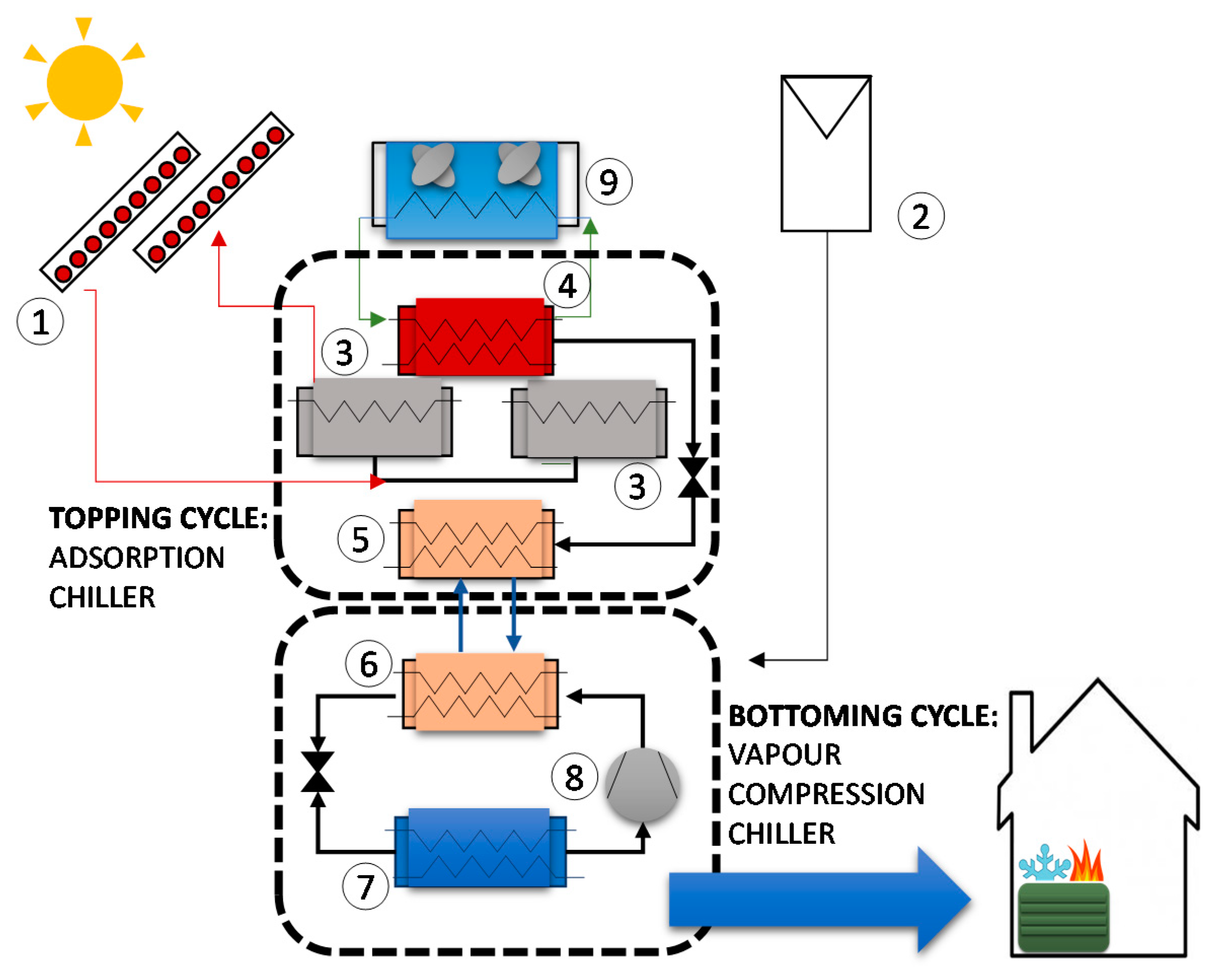
2. System Description

The sorption-compression system proposed is mainly meant for integrating different renewable sources at the building scale (e.g., solar thermal and PV). It is especially meant for operation in warm (e.g., Mediterranean) climates, to provide cooling energy at high efficiency. The overall system is depicted in Figure 1.

The core sub-system is composed by the cascading integration of an adsorption chiller (topping cycle) with a vapour compression chiller (bottoming cycle). When the solar energy is available, thermal energy, (1) in Figure 1, is used to drive the adsorber (3) of the adsorption chiller. The chiller comprises two adsorbers working in counter-phase, to continuously provide cooling on the evaporator (5) side, which cools down the condenser of the bottoming vapour compression chiller (6). The cooling effect to the end-user is provided by the evaporator on the vapour compression side (7). In this way, the heat from the vapour compression chiller is “pumped” to the adsorption chiller, which then discharges it to the ambient by condensing the refrigerant in (4) and dissipating it to the ambient (9). Thanks to this operation, the condensation of the vapour compression chiller is reduced compared to the ambient temperature. This allows reducing the pressure difference between evaporator (7) and condenser (6), limiting the energy consumption to drive the compressor (8). In this way, the cold is produced at high electric efficiency and it can be either directly delivered to the used or stored in a separated tank, for providing energy upon request. The flexibility of the system allows foreseeing different operating scenarios:

• if solar energy is not available, cold energy is produced directly from the vapour compression chiller, that can be directly connected to the dry cooler.
• If there is a mismatch between the solar availability and user demand, in order to exploit the renewable source, cold energy can be produced using the cascade system and stored in a sensible or latent cold storage.
• During winter, the heating demand of the building can be satisfied by direct connection to the solar collectors (if solar energy is available) or by the heat pump.
• Domestic hot water can be supplied by the solar collectors, coupled to a small water buffer or a back-up system (i.e., existing gas boiler in case of retrofitting).

To further enhance the share of renewables, electricity needed to drive the compression chiller can be supplied by PV panels when solar energy is available. It is then clear that the sizing and management of such a system are complex issues that require a model-based support.

3. Model Description: Adsorption Module

3.1. Generalities and Assumptions

For the case under study, a dynamic physical approach was chosen, which allows to describe the behaviour of a complex and innovative system under variable conditions, corresponding to the operation in a real environment. The open-source language Modelica was chosen [54]. It is a multi-domain, object-oriented and non-causal language, which guarantees a high reusability of the models created and gives the possibility of examining at the same time mechanical, thermal and electric systems. The model was implemented and post-processed within the Dymola software [55]. All the components models were realised using self-developed components as well as components from Thermocycle [56] and CoolProp libraries [57].

The layout of the model for the adsorption module is shown in Figure 2. It is based on the typical structure of a two-bed adsorption chillers, where two adsorbers, employing SAPO 34 as adsorbent material and water as refrigerant, are alternatively connected to a condenser and an evaporator by means of vacuum valves. Refrigerant flow from the condenser to the evaporator is guaranteed by an auxiliary expansion valve. All the components make use of fin-and-tube heat exchangers hydraulically connected to the heat sources and sinks providing the thermal energy for the operation of the components. Hence, the model developed for each component is made up of two sub-models: an equilibrium model and a heat exchange model. The equilibrium model is the vapour-liquid equilibrium (VLE) for the condenser and the evaporator and the adsorption equilibrium model in the adsorbers, i.e., the model linking the refrigerant uptake to the pressure and temperature distribution. Such an approach is similar to the one proposed in [34,58], that was validated against experimental data and proved to be a reliable tool to analyse adsorption systems.

The following assumptions were made:

• all components are lumped models with uniform properties;
• the heat transfer fluid inside the heat exchangers is incompressible;
• pressure drops inside the heat exchangers are constant;
• gravity is neglected;
• the thermal masses of vacuum vessels are neglected;
• there are no heat losses to the environment;
• there is no direct heat exchanger due to conduction between the components;
• there are no inert gases inside the closed volume.

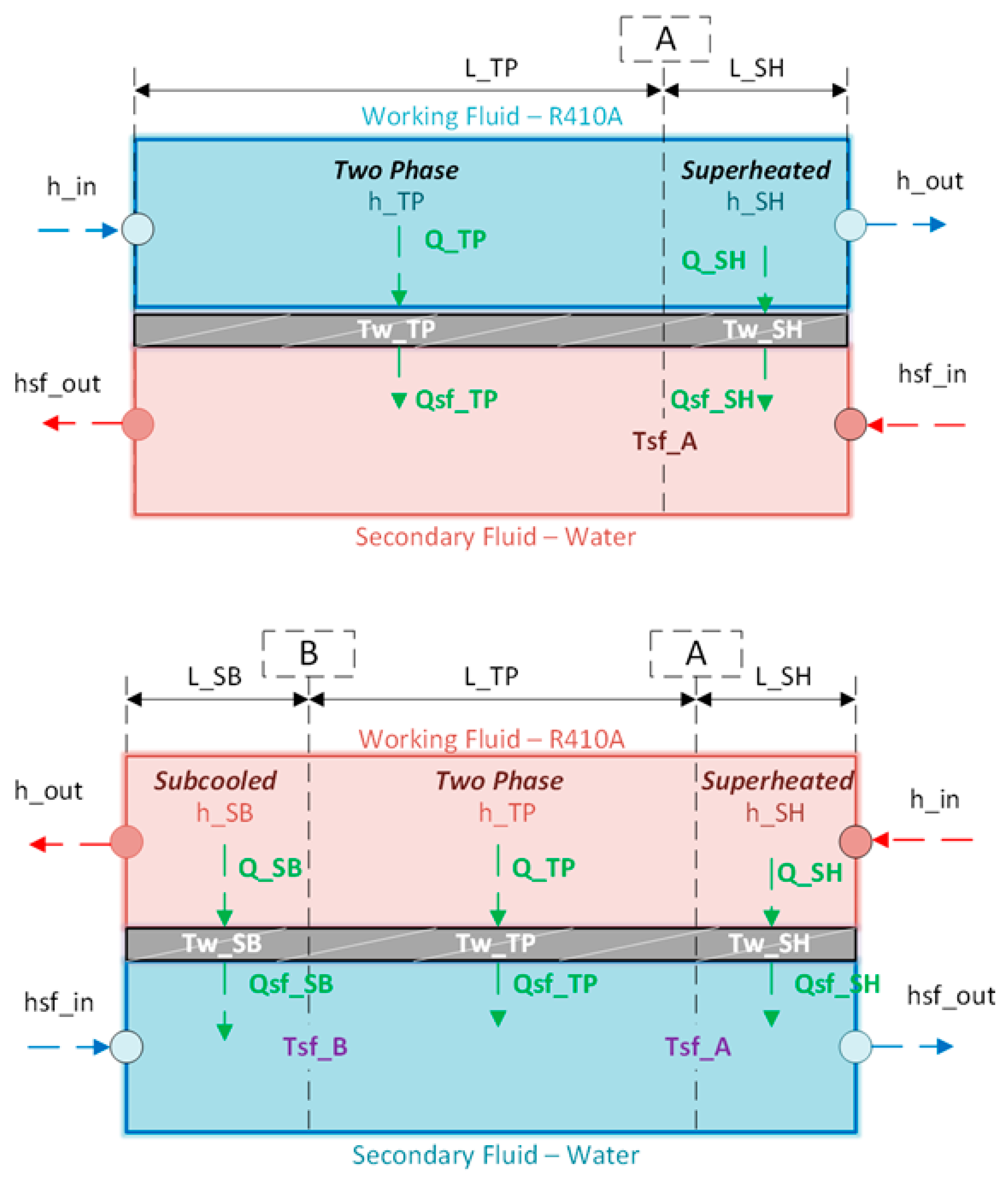
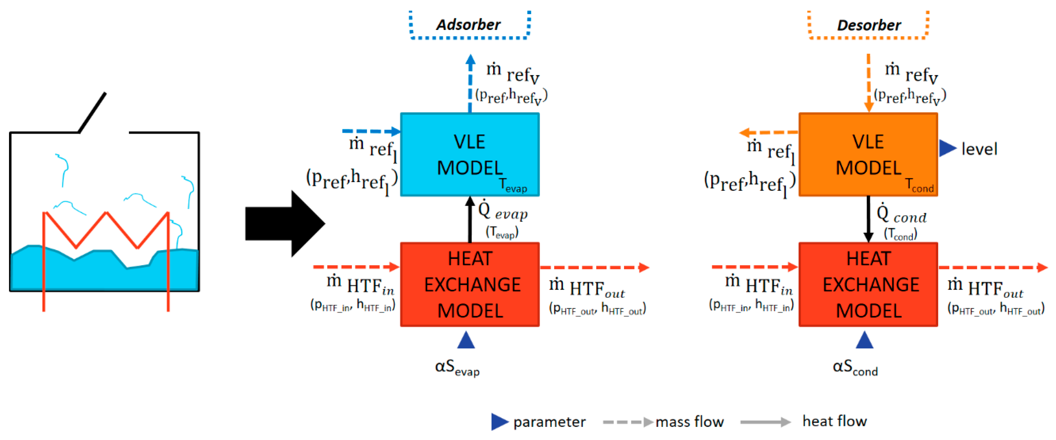
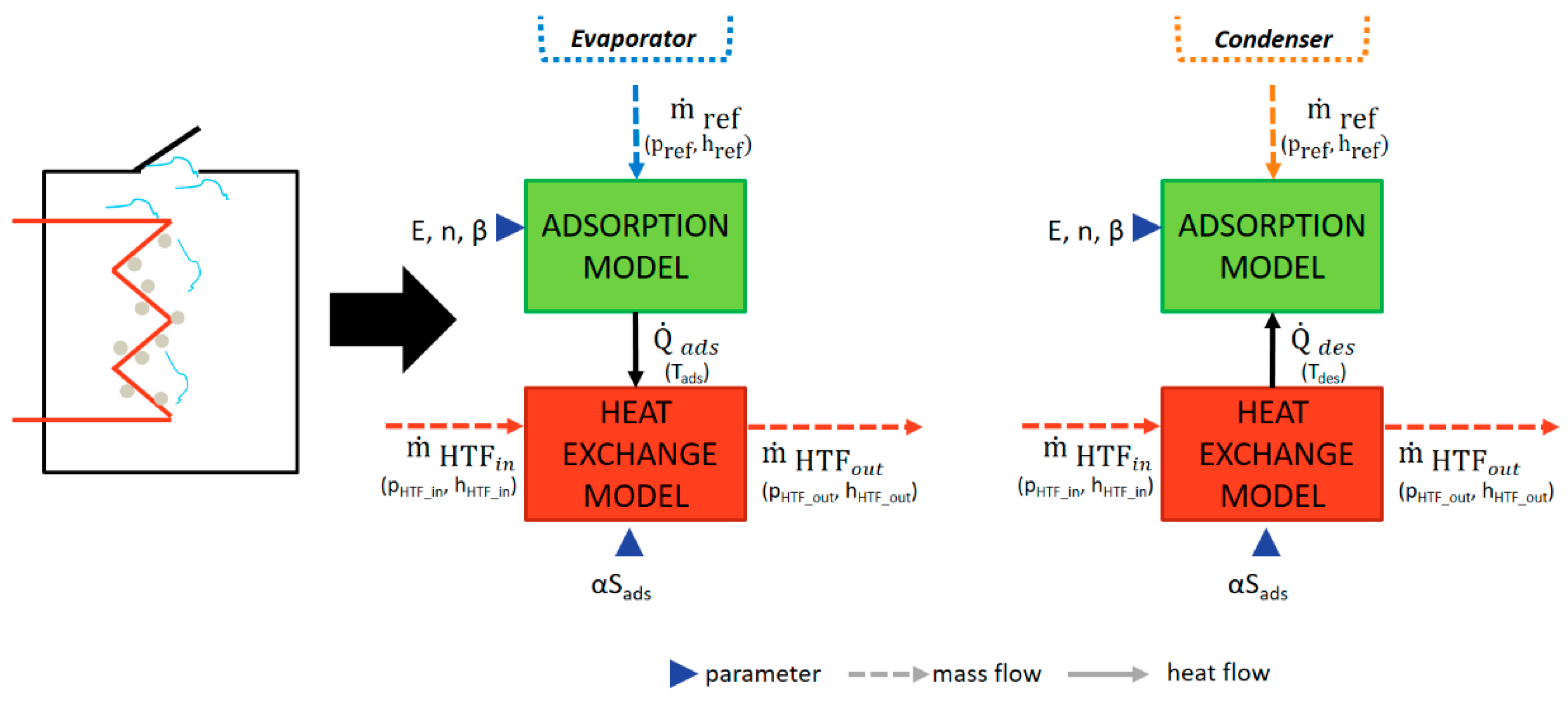
3.2. Heat Exchange Model

The heat exchange model is common to all the components in the adsorption model and is based on the 1D finite volume heat exchanger model present in the Thermocycle library. Indeed, a comparative analysis of the finite volume and moving boundary model implemented in the Thermocycle library for the simulation of heat exchangers was carried out in [59], proving that both approaches are reliable and allow for accurate simulations of different types of heat exchangers commonly used in energy systems. The model is based on mass, energy and momentum balance equations:

$${\dot{m}}_{HT{F}_{in}}+{\dot{m}}_{HT{F}_{out}}=0$$

(1)

$$p_{HT{F}_{in}}-p_{HT{F}_{out}}=∆p$$

(2)

$$\frac{dU}{dt}={\dot{H}}_{HT{F}_{in}}-{\dot{H}}_{HT{F}_{out}}+\dot{Q}$$

(3)

where:

$${\dot{H}}_{HTF}={\dot{m}}_{HTF}{h}_{HTF}$$

(4)

Heat transfer between the fluid inside the heat exchanger and the external environment is calculated using the following equation, where the heat transfer coefficient and heat transfer area are known parameters:

$$\dot{Q}=\alpha S\left(T_{fluid}-T_{metal}\right)$$

(5)

The enthalpy and the properties of the fluid are calculated from the CoolProp library as a function of local temperature/pressure conditions inside the heat exchanger.

3.3. Adsorption Model

The model for adsorption includes mass and energy conservation equations:

$${\dot{m}}_{re{f}_{in}}+{\dot{m}}_{re{f}_{out}}={\dot{m}}_{ref}$$

(6)

$$\left(m_{sorb}{c}_{p_{sorb}}+w·m_{sorb}{c}_{p_{ref}}\right)\frac{d{T}_{sorb}}{dt}={\dot{Q}}_{ads}+{\dot{m}}_{ref}{h}_{ads}-m_{sorb}{c}_{p_{sorb}}{T}_{sorb}\frac{dw}{dt}$$

(7)

In Equation (7), the terms on the left-hand side represent the sensible heat stored in the adsorbent, whereas the terms on the right-hand side represent the heat transferred through conduction and the mass exchange.

Different models are available to describe adsorption equilibrium, i.e., the uptake, w [kg/kg] (the amount of water adsorbed onto the material) as a function of temperature T_sorb, pressure p_ads in the adsorber, as well as the heat of adsorption [60]. Among them, for the SAPO-34 sorbent considered, the Dubinin-Ashtakov (DA) correlation was selected [61]:

$$w=w_0\exp \left[-{\left(\frac{A}{E}\right)}^n\right]$$

(8)

where w₀ and n are empirical constants and A is the adsorption potential:

$$A=-R{T}_{sorb}\log \frac{p_{ads}}{p_{sat}}$$

(9)

The flow rate of refrigerant adsorbed is a function of the uptake variation in time:

$${\dot{m}}_{ref}=m_{sorb}\frac{dw}{dt}$$

(10)

Uptake derivative depends on adsorption kinetics. A common approach to define is through the Linear Driving Force (LDF) [37,60,62]:

$$\frac{dw}{dt}=\beta \left(w_{eq}-w\right)$$

(11)

where the constant β is calculated as a function of the geometric characteristics of the adsorbent and of the diffusion coefficient D [63]:

$$\beta =\frac{15}{r^2{}_{sorb}}D$$

(12)

A schematic representation of the adsorber model, including the energy flows, the input and output parameters and variables is shown in Figure 3.

3.4. VLE Model

The two-phase refrigerant inside the evaporator and the condenser, which is exchanged with the adsorbers, is described by a vapour liquid equilibrium model including mass and energy balance equations in the form:

$$\frac{dm}{dt}={\dot{m}}_{re{f}_v}+{\dot{m}}_{re{f}_l}$$

(13)

$$\frac{dU}{dt}={\dot{H}}_v+{\dot{H}}_l+\dot{Q}$$

(14)

In the case of the condenser, the incoming fluid is vapour at the temperature of the adsorber and the outlet fluid is liquid having saturation enthalpy. Conversely, in the case of the evaporator, the incoming fluid is liquid at the temperature of the condenser and the outlet fluid is vapour having saturation enthalpy.

The term $\dot{Q}$ [W] represents the heat flow between the saturated refrigerant the surface of the heat exchanger:

$$\dot{Q}=\alpha S\left(T_{ref}-T_{metal}\right)$$

(15)

All the properties of the refrigerant in the liquid and vapour state are calculated from CoolProp library.

A schematic representation of the evaporator/condenser models, including the energy flows, the input and output parameters and variables are shown in Figure 4.

The equations for the auxiliary components and the parameters used in the modelling are described in Appendix A.

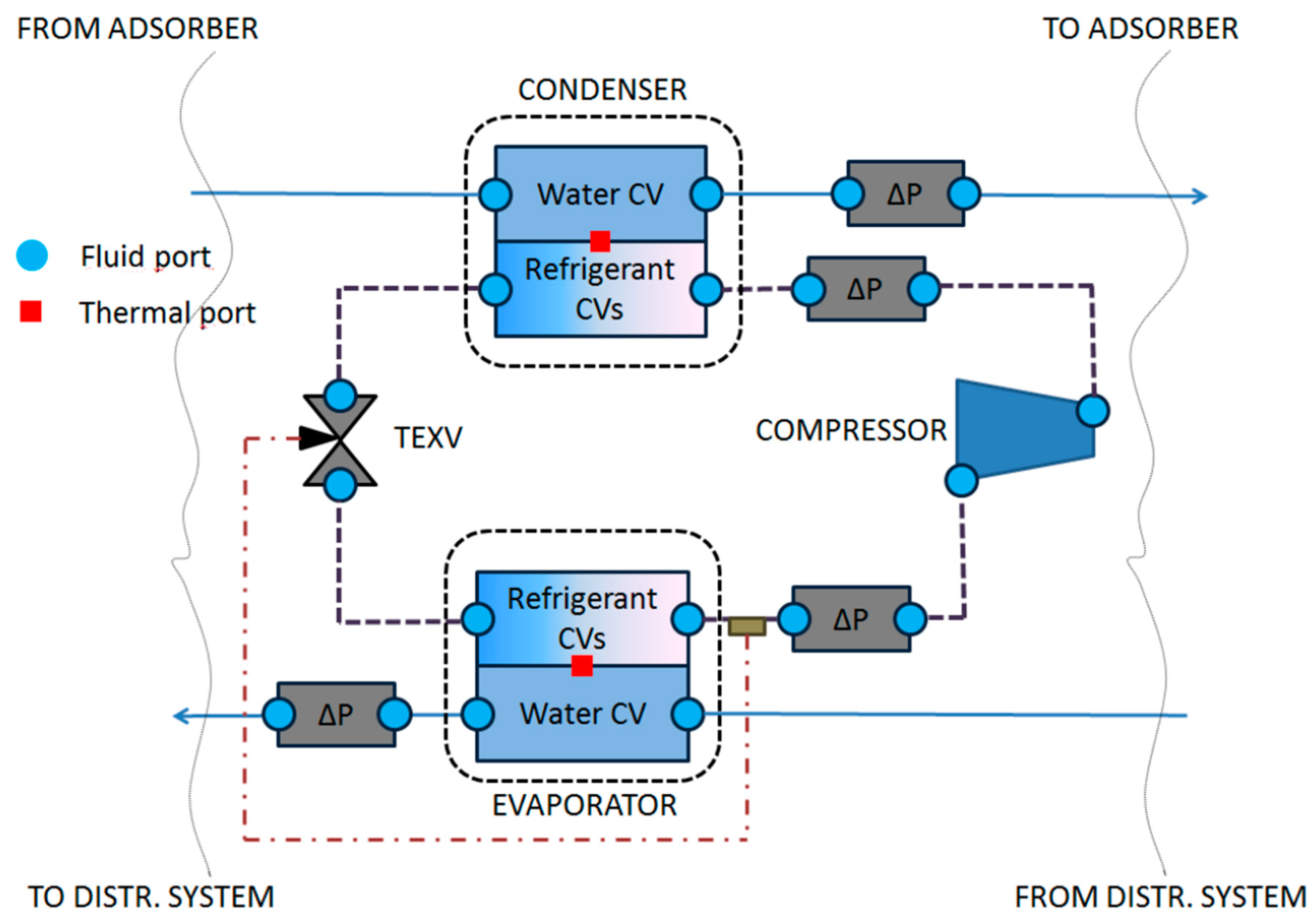
4. Model Description: Compression Chiller

4.1. Assumptions

The model for the compression chiller is based on a commercial water to water vapour compression chiller, using R410A as working fluid. It basically consists of four components, namely the two heat exchangers (evaporator and condenser), the compressor and the expansion valve. Fully dynamic models have been developed for the heat exchangers, whereas off-design steady state models were used for the compressor and the valve, which is a common practice in literature [17,56]. The operation of the Thermostatic Expansion Valve (TEXV), which ensures a degree of superheating at the inlet of the compressor by adjusting the refrigerant flow rate, was modelled by means of a PI controller. For validation and sizing purposes, only the operation in cooling mode (i.e., as a chiller) is considered, but the model already allows for switching also to heating mode. Since there is not a 4-way valve included in the refrigerant loop of the heat pump, heating or cooling operation can be selected by swapping the hydraulic circuits of the evaporator and the condenser, using four 3-way valves. The general assumptions made for the development of the components are:

• All components are lumped, with constant properties.
• One dimensional flow in each component with uniform velocity profile.
• No pressure loss inside the heat exchangers. Instead, lumped pressure loss models in both refrigerant and water pipelines were employed.
• Heat losses to the ambient are neglected for every component.
• Neglected dynamics for the compressor.
• Constant electromechanical efficiency of the compressor motor.
• Existence of subcooling and superheating at the outlet of the condenser and the evaporator respectively.
• Heat transfer coefficients vary with their nominal values according to the mass flow rate to nominal mass flow rate ratio.

All the models make use of self-developed components, based on the version 2.1 of the ThermoCycle library and the CoolProp thermodynamic properties software, together with standard ThermoCycle components.

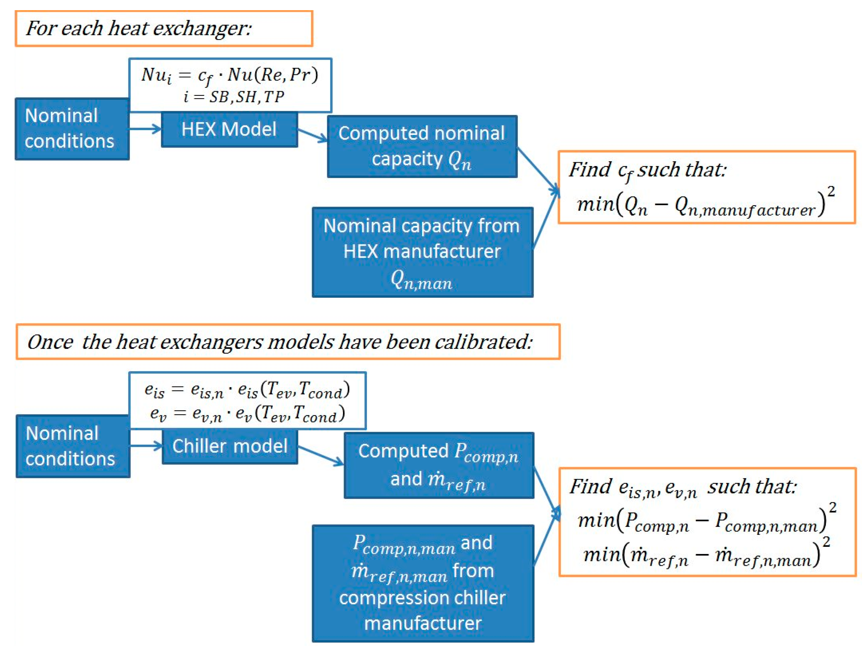
4.2. Heat Exchangers Models

The modeling approach followed for the heat exchangers is the Moving Boundaries technique. Moving boundaries models are generally faster compared to finite volume implementations, without losses in modelling accuracy [64]. The main drawback of the Moving Boundaries approach is the definition of start-up and shut-down procedures: using the classical Moving Boundary formulation, the possible phase zones of the refrigerant and the associated control volumes—i.e., superheated (SH), two phase (TP) and subcooled (SB)—have to be predefined during the model development. As a result, the simulation of the start-up process of the heat pump, which for example starts with the evaporator being totally in the two phase mode and ends with the creation of a superheating zone, is not possible. Switching between various Moving Boundaries implementations, leading to a Switching Moving Boundary model, seems to allow the examination of the heat pump operation during start up and shutdown procedures [65,66,67], but since in this work attention was given mainly to the continuous operation of the cascading hybrid system under varying conditions, the classical but simpler moving boundary models described in [68] by Willatzen et al. was employed. In the next section, a general overview of the methodology is presented, while the complete set of equations is included in the Appendix A and Appendix B. For a detailed description of the methodology, the reader is referred to [68].

Each of the heat exchangers was divided in control volumes (CVs) according to the expected refrigerant phases (TP-SH for the evaporator and SH-TP-SB for the condenser—see Figure 5). In each control volume the heat and mass balances are expressed with regards to the control volume’s length, by means of the Leibnitz’s rule. For each control volume, enthalpy and pressure are selected as state variables, by expressing the time derivative of each thermodynamic property to $\frac{dp}{dt}$ and $\frac{dh}{dt}$ using the chain rule. As an example, the following equation gives the derivative of the density in the SH control volume:

$$\frac{d{\rho }_{SH}}{dt}=\left[{\left(\frac{\partial {\rho }_{SH}}{\partial p}\right)}_h+\frac{1}{2}{\left(\frac{\partial {\rho }_{SH}}{\partial h}\right)}_p\frac{d{h}_v}{dp}\right]\frac{dp}{dt}+\frac{1}{2}{\left(\frac{\partial {\rho }_{SH}}{\partial h}\right)}_p\frac{d{h}_{in} }{dt}$$

(16)

The mean void fraction, used to calculate the average node properties in the two phase control volume, was considered constant for both heat exchangers, to a value close to its nominal one, which was calculated according to the homogeneous definition [69]:

$$\gamma ={{\displaystyle \int }}_{x_0}^{x_L}\frac{\frac{x}{{\rho }_v}}{\frac{x}{{\rho }_v}+\frac{1-x}{{\rho }_l}}dx$$

(17)

This simplification is widely used in this kind of models, without loss of accuracy [68], though an analytical expression for the mean void fraction and its time derivative is needed in switching moving boundaries implementations.

As an enhancement to the original equations proposed by Willatzen- and similarly to the standard moving boundary implementation in ThermoCycle- the heat transfer between the primary and the secondary fluid is calculated by means of ε-NTU method, instead of calculating it using the temperature difference between the corresponding cells. The method was applied twice in each volume, once for the water and once for the refrigerant stream, utilizing the wall temperatures.

For example, the heat flow in the superheated CV of the refrigerant can be expressed using the mean wall temperature by means of the following equation:

$${\dot{Q}}_{SH}=c_{p,SH}\frac{{\dot{m}}_A+{\dot{m}}_{in}}{2}\epsilon \left({{\rm T}}_{wallSH}-T_{in}\right)$$

(18)

For the complete set of equations used in the models of the components, the reader is referred to Appendix B.

4.3. Compressor Model

The chiller modeled makes use of a hermetic scroll compressor, which was modeled using a steady state approach, since the dynamic phenomena of the compressor can be considered as negligible compared to the ones imposed by the heat exchangers. The hermetic compressor includes both the open drive scroll compressor and the electric motor. The open drive scroll compressor model is derived from the standard compressor model included in ThermoCycle library, while the motor model is a modified version of the standard ElectricDrive of the library.

The isentropic and volumetric efficiencies were expressed as polynomials of the evaporation and condensation pressures, similar to the ones proposed in the EN12900 [70]. Hence, the isentropic efficiency $e_{is}$ and the volumetric efficiency of the compressor $e_{vol}$ can be derived from an equation of the type:

$$\begin{gathered} e_{is}=e_{is,n}·(C_0+C_1·T_{ev}+C_2·T_{cond}+C_3·T_{ev}^2+C_4·T_{ev}·T_{cond}+C_5·T_{cond}^2+C_6·T_{ev}^3 \\ +C_7·T_{cond}\ast T_{ev}^2+C_8·T_{ev}·T_{cond}^2+C_9·T_{cond}^3) \end{gathered}$$

(19)

The coefficients were calculated using the performance data of a typical commercial compressor of the same power range and with the same working fluid, while the nominal values for both the volumetric ($e_{v,n}$) and isentropic ($e_{is,n}$) efficiencies were used to adapt this equation to the specific compressor and were defined using the chiller’s manufacturer data.

As a result, the mass flow rate transferred by the compressor is calculated using the following equation:

$${\dot{m}}_{ref}=e_{vol}\frac{rpm·V_s·{\rho }_{SU}}{60}$$

(20)

where ${\dot{V}}_s$ the swept volume of the compressor.

The enthalpy at the outlet of the compressor is calculated using the definition of the isentropic efficiency:

$$h_{out}=h_{in}+\frac{\left(h_{out,is}-h_{in}\right)}{e_{is}}$$

(21)

The shaft power needed for the compression is calculated as:

$$W_{shaft}={\dot{m}}_{ref}\left(h_{out}-h_{in}\right)$$

(22)

The motor model, being coupled with the scroll compressor, is used for the calculation of the electric power consumption of the machine, by means of a constant value for the efficiency, considered equal to 0.93. Besides, the model was modified in order to take into account the electromechanical slip of an induction motor, defined as:

$$slip=\frac{rp{m}_{sync}-rpm}{rp{m}_{sync}}$$

(23)

where $rp{m}_s$ is the synchronous speed. Since the motor has 2 magnetic poles, the synchronous speed in a common 50 Hz grid is $rp{m}_s=3000 \mathrm{RPM}$, while the value of the slip was assumed as constant and equal to the nominal one.

4.4. Thermostatic Expansion Valve model (TEXV)

The thermostatic expansion valve model is based on the standard Valve component of the ThermoCycle library, controlled by a PI controller which maintains the superheating at a desired value and models the valves dynamics, caused by the spring action.

The mass flow rate through the valve is calculated form the pressure drop using the following expression:

$${\dot{m}}_{ref}=S·\sqrt{2·{\rho }_{in}·\Delta p}$$

(24)

where S is the area of the orifice inside the valve. S is changing linearly with the control signal, so:

$$S=y·S_{full}$$

(25)

The fluid flow through the valve is assumed adiabatic, so the expansion is isenthalpic. The superheating of the fluid exiting the evaporator is calculated in real time during simulations as the different between the evaporation temperature and the refrigerant’s outlet temperature. The gains of the PI controller were set in order to achieve a fast but smooth operation and avoid oscillations

The simulation of the compression chiller is completed by lumped pressure drops elements and the models of the valves, that are described in Appendix B. All the parameters used in the simulations are also listed in the Appendix A and Appendix B, while the schematic layout of the compression chiller is shown in Figure 6.

5. Model Validation

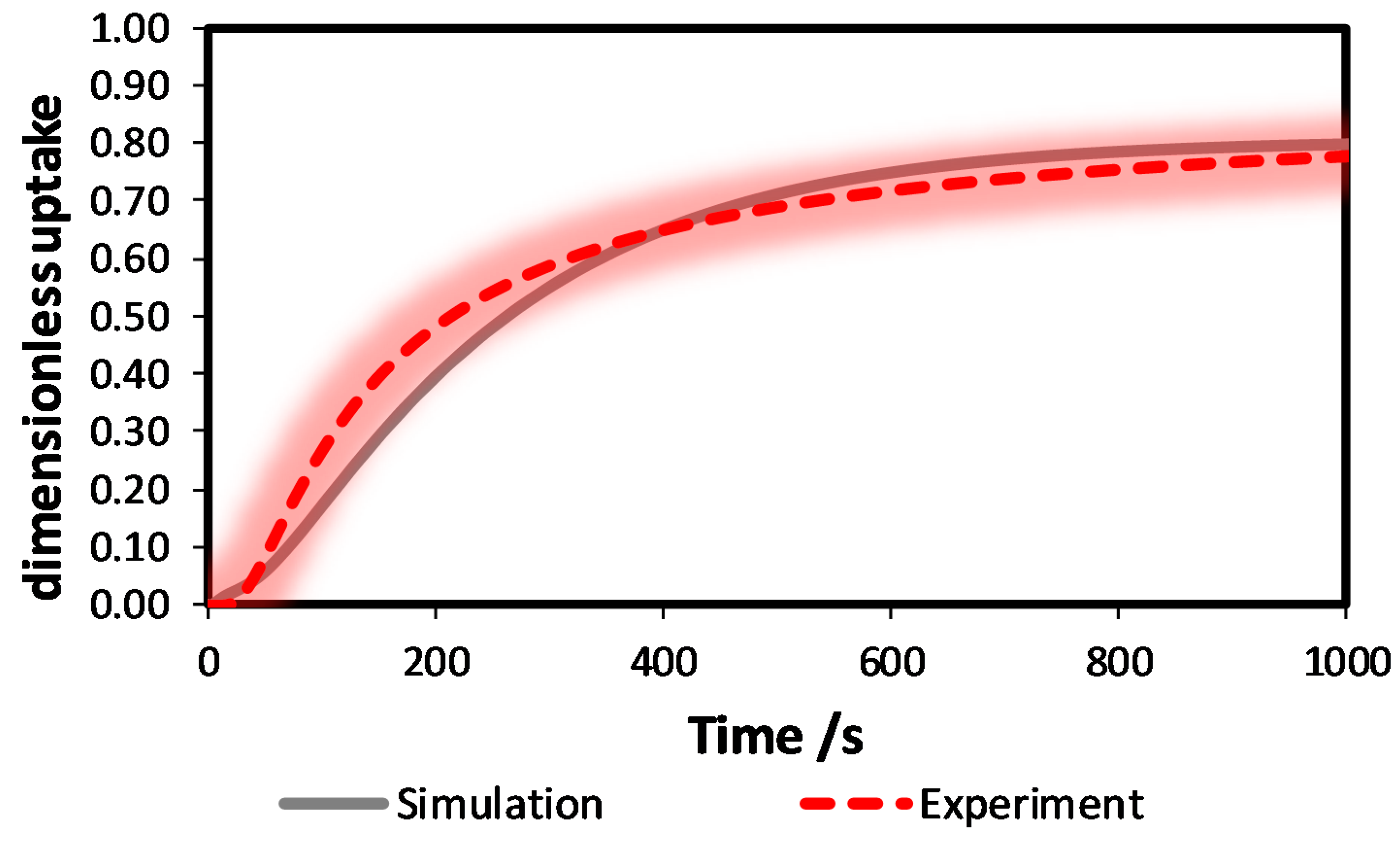
5.1. Adsorption Module

In order to validate and calibrate the model of the adsorption chiller, similarly to what described in [71], the results of a simulation for the adsorber were compared to the results of a test made with a gravimetric Large Temperature Jump apparatus, that allows to record the variation in the weight (and hence the uptake) of a small-scale adsorber when subjected to a sudden change of temperature. Indeed, such kind of tests are of the uttermost importance in the selection of the adsorber, in terms of layout of the heat exchanger and grain size of the adsorbent [72,73] and therefore represent an essential benchmark for the model developed, guaranteeing that the model can be used for optimization and sizing of a complete hybrid system.

For validation purposes, results with AQSOA FAM Z02^® (by Mitsubishi Chemical Corporation, Tokyo, Japan), with grain size 0.710–0.800 mm, published in [74], were used. The results are shown in Figure 7, where the temporal evolution of the dimensionless uptake for simulation and experiments are compared. The dimensionless uptake represents the ratio between the uptake at each instant and the uptake at equilibrium in the temperature-pressure conditions tested. Commonly, the value of time needed to complete 63% of the adsorption reaction and the time needed to reach 80% of maximum uptake are used for sizing and evaluation analysis on dynamic properties of sorbents. It is possible to conclude that the model can actually reproduce with good accuracy such conditions, thus being a useful tool. The maximum deviation with experiments is around 7.5%, which is within uncertainty of measurement and is concentrated in the part of the curve with low loading, where the experimental conditions are affected by several external factors, such as vibrations due to the switching of the hydraulic circuits and so on.

5.2. Compression Chiller

The free parameters of the compression chiller model were tuned based on the values specified by the chiller and heat exchangers manufacturers around their nominal operating point: A constant correction factor was multiplied with the constant terms of the heat transfer correlations of each heat exchanger, thus defining one free parameter per heat exchanger, which was calculated iteratively in order to minimize the deviation between the model output and the heat exchanger manufacturer data in nominal conditions. Next, the nominal values for the isentropic and volumetric efficiencies, $e_{is,n}$ and $e_{v,n}$ respectively, were identified iteratively in order to achieve the best fitting to the data provided by the chiller manufacturer around its nominal operating point. In each case, the iterative procedure was implemented in Dymola, utilizing the Model Calibration Toolbox. The whole procedure is depicted in Figure 8:

Once being calibrated on the nominal conditions, the model was validated by using a data set of 24 operating points provided by the chiller manufacturer, including the inlet water temperatures and heat capacities of the evaporator and the condenser as well as the compressor electric power consumption. The evaporator inlet water temperatures of the dataset range from 10 °C to 20 °C while the condenser inlet water temperatures from 20 °C to 40 °C. A fixed ΔΤ equal to 5K is considered for the water streams in both heat exchangers, which is the common reference for the Eurovent certification programme [75].

The results of the comparison of the model to the performance data are summarized in Figure 9, where the relative errors on the evaporator cooling capacity and the EER are presented for different evaporator and condenser water inlet temperatures. The conditions simulated and compared with performance data are marked with black dots. The relative error is calculated as:

$$Relative Error(\%)= \frac{{\xi }_{model}-{\xi }_{dataset}}{{\xi }_{dataset}}·100$$

(26)

The EER of the chiller is defined as the ratio between the cooling power at the evaporator ${\dot{Q}}_{ev}$ and the electricity consumption of the compressor:

$$EER=\frac{{\dot{Q}}_{ev}}{P_{comp}}$$

(27)

Figure 9 shows that the model predicts fairly well the performance data of the compression chiller: while the maximum deviation is around 3% for the evaporator capacity and around 5.5% for the EER. Moreover, it is clear that in the operating range that is of particular importance for the cascaded system simulation (cooling mode with low condensing temperatures due to the operation of the sorption chiller), the model has its best accuracy.

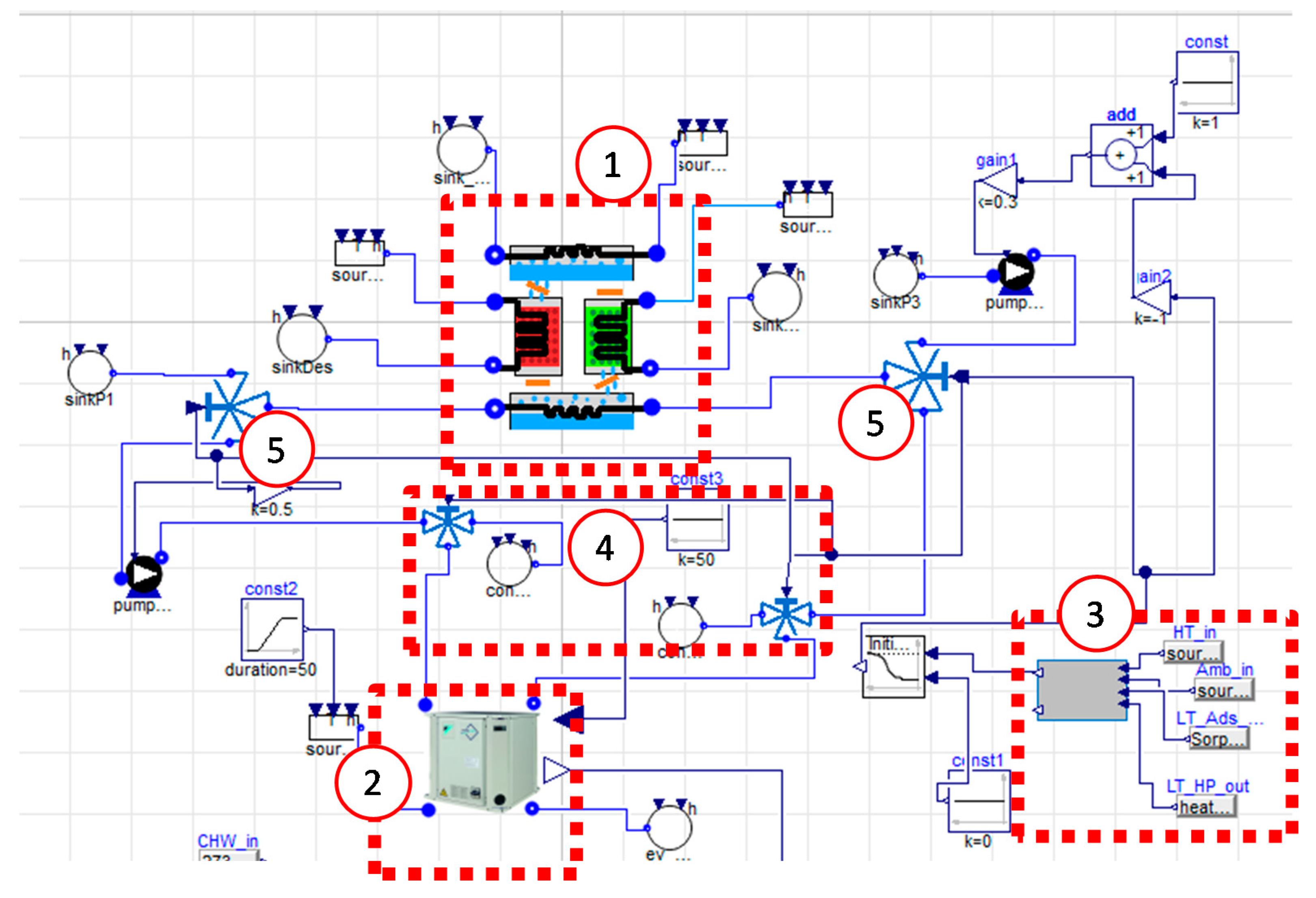
6. Hybrid System Integrated Model: Results

The models previously described were integrated, in order to reproduce the system configuration, as described in Section 4. The layout of the integrated model, as taken from the simulation software, is shown in Figure 10, where the main components are highlighted.

In addition to the main components previously presented, the model includes a control unit, where the basic controls for the correct operation of the system under dynamic conditions are codified, and 3-way hydraulic valves, used to control the operating mode of the hybrid system. Indeed, under some conditions, even under the presence of cooling load, the combined cascade operation of the two cycles is not possible or not convenient. Under these circumstances, the compression chiller is directly connected to the heat rejection circuit. The following main conditions were applied as basic rules to run the adsorption module:

• the temperature of the heat source is higher than a user-defined value (in the present case, 75 °C);
• the temperature in the chilled water circuit (evaporator secondary circuit) of the adsorption unit is lower than T_amb − 5 °C, the condition under which direct connection of the compression unit with the external sinks becomes more favorable.

The integrated model developed was then used to verify the operation of the system under realistic dynamic conditions and as starting point for a technical analysis, useful for design purposes. All the simulations carried out were solved using the Radau solver in Dymola with 0.001 tolerance and a time step of 1 s.

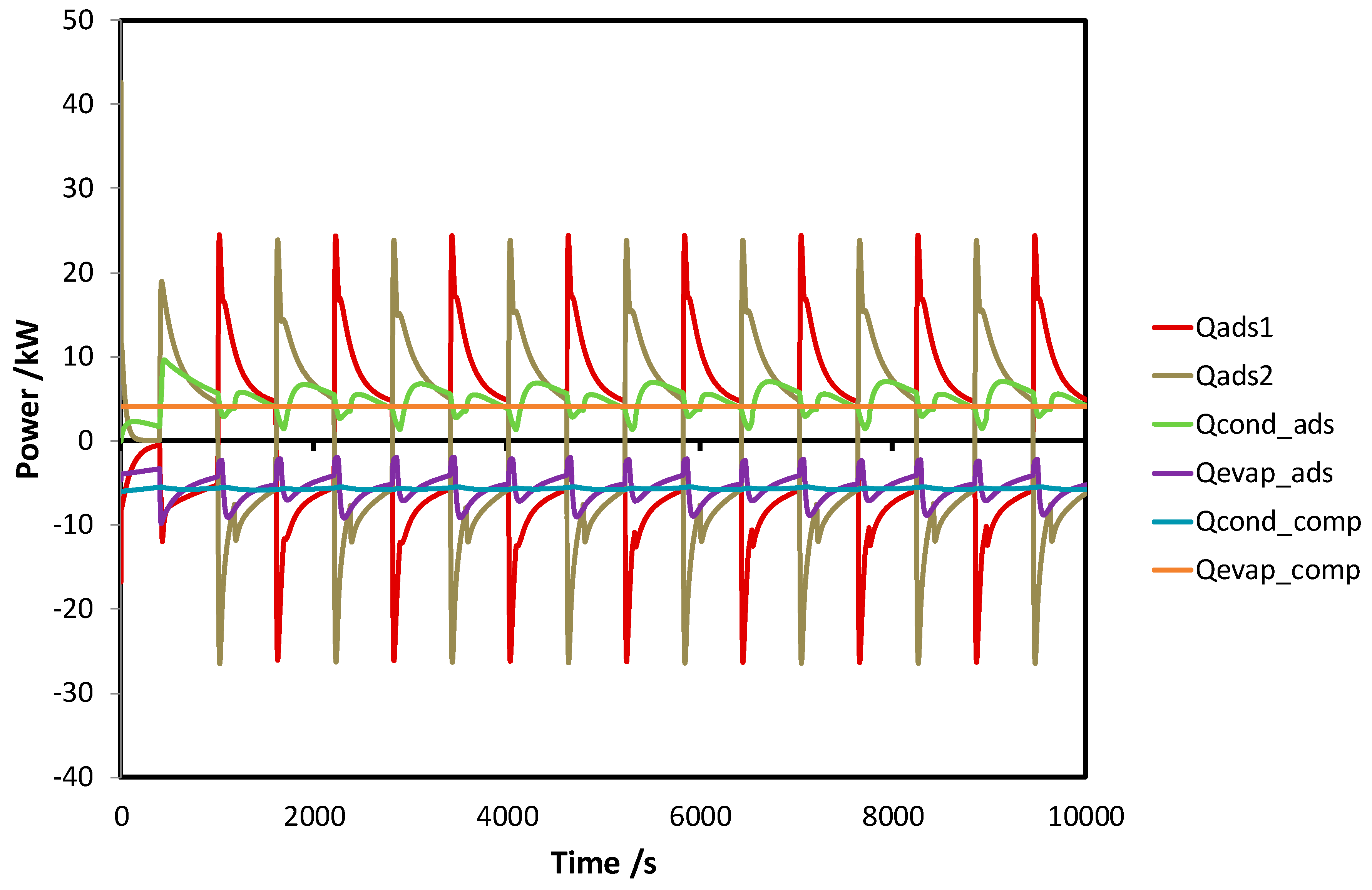
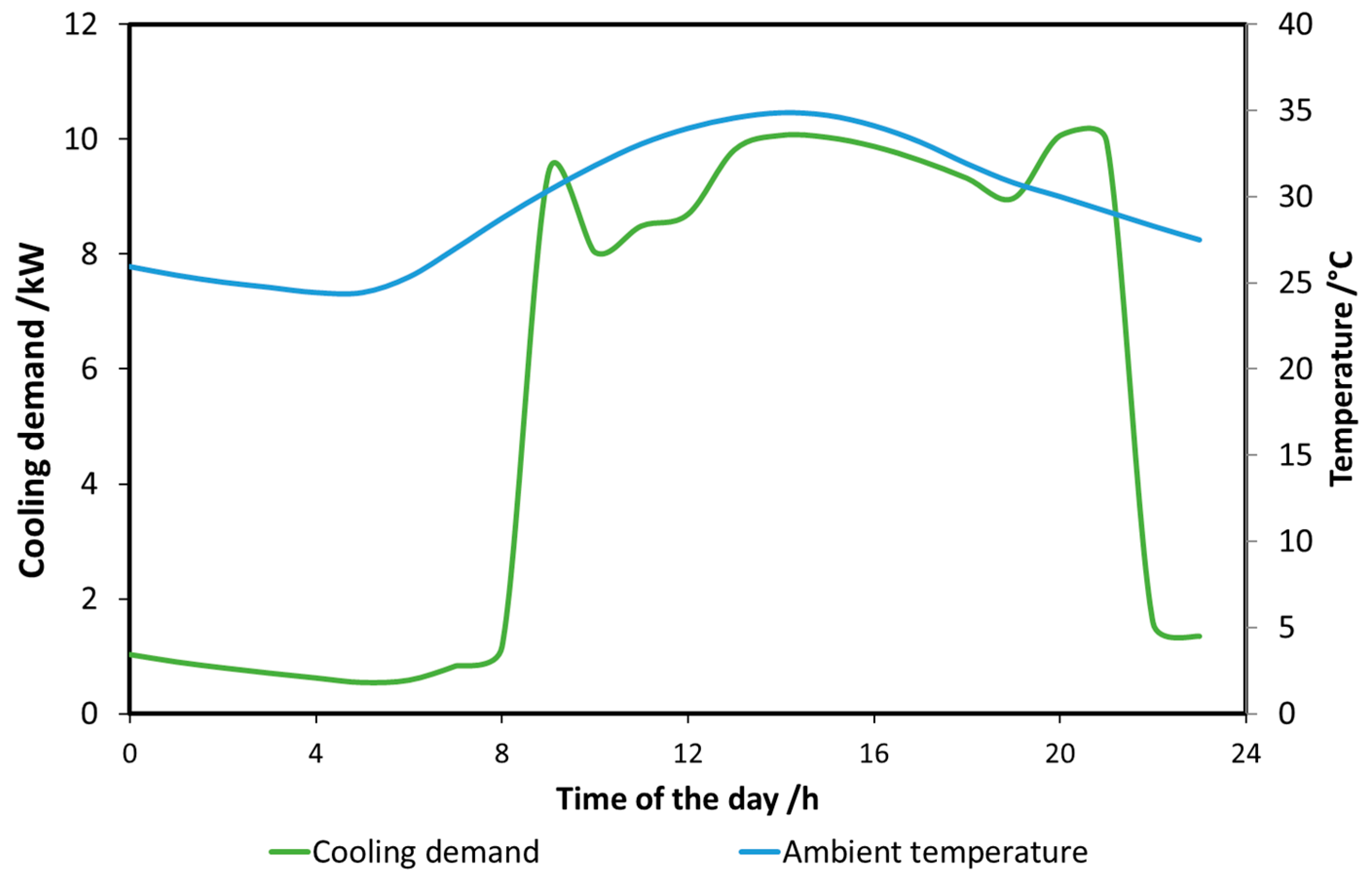
6.1. Results in Dynamic Conditions

The operation of the system in dynamic conditions was simulated considering the installation in a residential building in Aglantzia (Cyprus) that will be one of the pilot sites for the HYBUILD concept. To this aim, a reference day was selected, corresponding to ASHRAE design conditions for Cyprus (month of August, peak temperature of 35 °C). The cooling demand and ambient temperature for the reference day are shown in Figure 11. Such data were fed into the model as a text file instead than by coupling the developed model with a building model, since the main scope of the analysis was to define the feasibility in the application of the integrated model developed under dynamic conditions. Further evaluations by direct connection of the hybrid system to a simplified building models will be carried out in the future, to assess the performance of the system. The cooling demand of the reference building was calculated by the pilot plant owner and used as a benchmark of the robustness of the model developed.

The results of the simulations run from 9 am to 15 pm are shown in Figure 12 and Figure 13. It is possible to notice the typical discontinuous behaviour of the adsorption chiller in all circuits, with the most marked variability on the evaporator circuit of the sorption module (light and dark green lights in Figure 11). This evolution is due to the combined effect of the cyclic operation of the chiller and the increase in the temperature of the circuit due to the condensation heat coming from the vapour compression chiller. What can be noticed is the sensible reduction in the inlet temperature to the condenser of the vapour compression chiller (light green line): despite the periodic rising, the average is below 20 °C, thus reducing the temperature lift of the unit more than 10 K compared to the ambient temperature.

Instead, Figure 13 shows the powers in the different components of the adsorption module and the vapour compression chiller. It is possible to notice that the power in the condenser of the vapour compression chiller corresponds to the average power from the evaporator of the adsorption module. Moreover, at each phase change there is a peak in the power absorbed/released from the adsorbers, due to the sensible heat and sorption heat of the material. Finally, it is worth mentioning that the power from the compression chiller evaporator remains constant and thus unaffected from the discontinuities in the condenser side, proving the stable operation of the cascading system from the end user point of view.

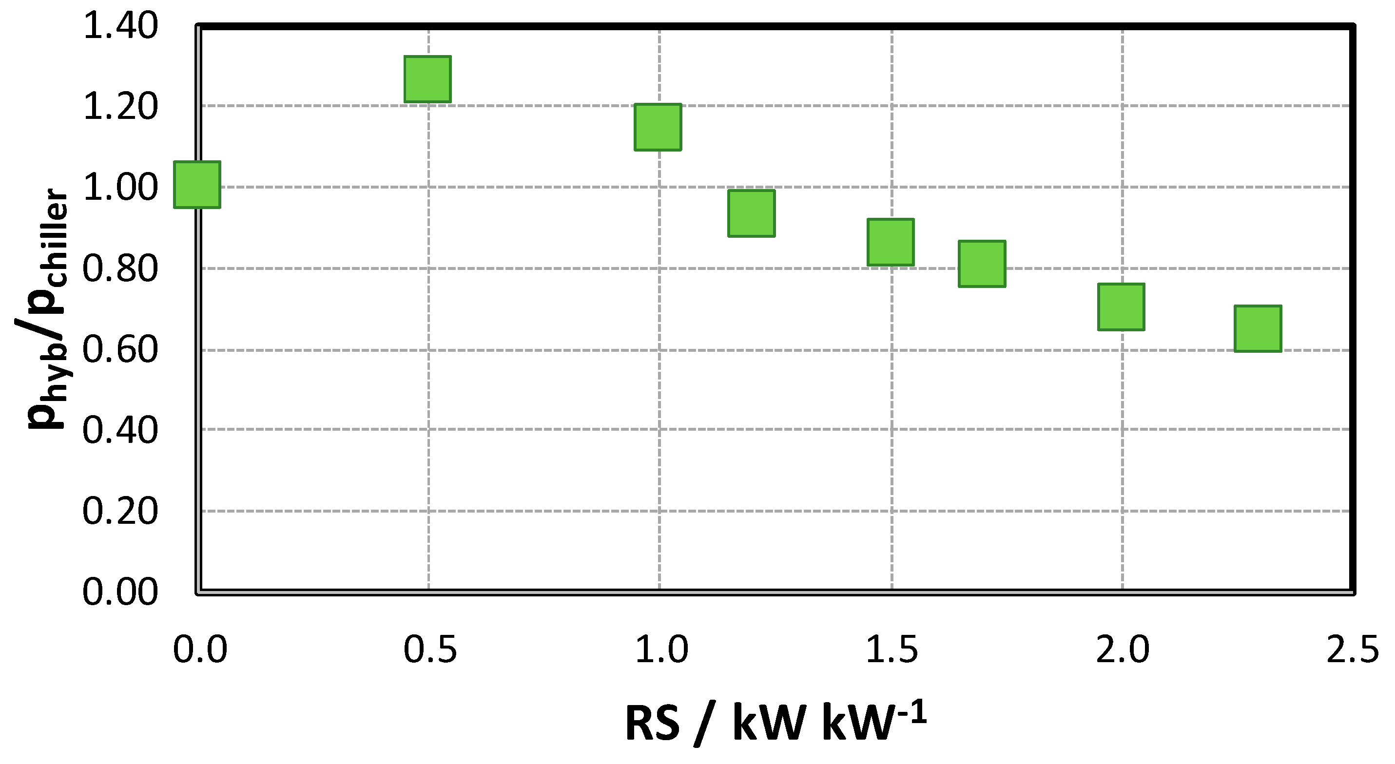
6.2. Sensitivity Analysis

After evaluation under realistic operation, the model developed was used for a sensitivity analysis, suitable to define some of the design and sizing parameters of the components. One of the parameters evaluated is the relative size of the adsorption and compression units:

$$RS=\frac{{\dot{Q}}_{nom,ads}}{{\dot{Q}}_{nom,chiller}}$$

(28)

The nominal power of the adsorption chiller is defined as the power that the unit can deliver when not working in cascade, in the following conditions: 90 °C heat source temperature, 30 °C condensation temperature and 18 °C evaporation temperature. Instead, the nominal power of the vapour compression chiller is the cooling power declared by the producer. For the present case, since the application considered is the residential one, a nominal power of 13 kW of the vapour compression chiller was selected, which is the minimum one that the producer can supply.

The parameter used as benchmark for the sensitivity analysis is the ratio between the operating pressure of the condenser in the vapour compression chiller when in hybrid configuration and the operating pressure of the condenser in the vapour compression chiller when in working as a single unit:

$$\kappa =\frac{p_{hyb}}{p_{chiller}}$$

(29)

The results of the analysis are reported in Figure 14. The external conditions for the operation of the hybrid and the compression chiller alone were: 90 °C constant heat source inlet to the adsorption unit, 30 °C constant inlet to the condenser (in the adsorption unit for a hybrid configuration, or of the compression chiller for stand-alone operation) and 12 °C constant inlet to the evaporator of the compression chiller. Nominal flow rates were considered in all the circuits.

The results are averaged over 3 h of operation. The results show that undersizing the adsorption unit (i.e., 0.5 < RS < 1.2) is detrimental to the operation of the compression chiller: indeed, since the power supplied by the adsorption unit is not enough to dissipate the condensation heat of the compression chiller, the operating pressure of the condenser in this latter unit is up to 30% higher than in stand-alone operation. On the other hand, oversizing the adsorption unit (i.e., RS > 2), does not give a significant advantage in terms of operating pressure (and therefore electric savings), and can even lead to problematic operation due to the risk of reducing too much the operating pressure during the first seconds of each adsorption phase, when the evaporation power is maximum.

6.3. Applications of the Model

The results reported above demonstrate that the model developed is capable of describing the system analysed under dynamic conditions. However, as demonstrated in Section 6.2, it is also useful for a technical evaluation on the system and its sub-components. One of the main advantages of the approach proposed is the possibility of easily calculate the performance of the overall hybrid system under several defined boundaries (i.e., part load ratio and external temperatures). The data collected in such a way can be used to derive:

(a)

lookup tables, useful for example as input data in a TRNSYS or Energy Plus model for annual energy evaluation or to test different control strategies at system level;

(b)

analytical equations, correlating the EER/COP to the operating conditions. Such equations can be re-used in a simplified model to be applied for optimization of control strategies.

Indeed, in literature, several model-based approaches are described for the definition of smart control strategies of air conditioning systems. They make use of simplified correlations between operating parameters and system performance indicators [76], thermodynamic models of the components [77], equivalent thermal parameters [78] or more advanced couplings of dynamic models and optimization methods, i.e., by means of genetic algorithms [79]. The proposed model can, with limited effort, be used to derive the simplified correlations needed for such applications or, exploiting the a-causality of the language and the possibility to exchange the model through FMUs, thus configuring as a useful tool also for the evaluation of control strategies.

7. Conclusions

In the present paper, the model of a hybrid adsorption-compression system, comprising a topping adsorption cycle and a bottoming vapour compression cycle is described. The system modelled allows efficient production of cooling the dynamic model of the system was realised in the Modelica language using the commercial software Dymola and open source libraries, i.e., the Thermocycle library and the Cool Prop library. Self-developed components for the adsorbers, condenser and evaporator in the adsorption and compression chiller unit were integrated with existing models, in order to replicate the layout of the real hybrid system. The model was validated against experimental data of the adsorber and performance data of the compression chiller, showing deviations lower than 5% and therefore demonstrating to be a reliable tool. It was subsequently used to verify the operation of the system under realistic dynamic conditions and as starting point for a technical analysis, useful for design purposes. A sensitivity analysis was carried out to identify the optimal relative size of the two units, with respect to nominal value: it was found out that, for properly exploiting the benefits of the proposed cascade configuration, the adsorption unit should have a nominal cooling power at least 50% higher than the nominal cooling power of the compression chiller. The results obtained indicate that the model developed is suitable for evaluation, without excessive computational effort, of the performance of the system, as well as a valid mean for technical analysis. The peculiarity of the language adopted and the open source libraries chosen allow also for a high reusability of the models, that can be easily adapted to different configurations and hybrid systems.

References

1. European Commission. Directive 2010/31/EU of the European Parliament and of the Council of 19 May 2010 on the Energy Performance of Buildings; European Commission: Brussels, Belgium, 2010. [Google Scholar]
2. Gullbrekken, L.; Grynning, S.; Gaarder, J.; Gullbrekken, L.; Grynning, S.; Gaarder, J.E. Thermal Performance of Insulated Constructions—Experimental Studies. Buildings 2019, 9, 49. [Google Scholar] [CrossRef]
3. Rony, R.; Yang, H.; Krishnan, S.; Song, J.; Rony, R.U.; Yang, H.; Krishnan, S.; Song, J. Recent Advances in Transcritical CO2 (R744) Heat Pump System: A Review. Energies 2019, 12, 457. [Google Scholar] [CrossRef]
4. Bee, E.; Prada, A.; Baggio, P.; Bee, E.; Prada, A.; Baggio, P. Demand-Side Management of Air-Source Heat Pump and Photovoltaic Systems for Heating Applications in the Italian Context. Environments 2018, 5, 132. [Google Scholar] [CrossRef]
5. Dengiz, T.; Jochem, P.; Fichtner, W. Demand response with heuristic control strategies for modulating heat pumps. Appl. Energy 2019, 238, 1346–1360. [Google Scholar] [CrossRef]
6. Pospíšil, J.; Špiláček, M.; Kudela, L. Potential of predictive control for improvement of seasonal coefficient of performance of air source heat pump in Central European climate zone. Energy 2018, 154, 415–423. [Google Scholar] [CrossRef]
7. Millar, M.-A.; Burnside, N.; Yu, Z. District Heating Challenges for the UK. Energies 2019, 12, 310. [Google Scholar] [CrossRef]
8. Zhang, L.; Li, F.; Sun, B.; Zhang, C.; Zhang, L.; Li, F.; Sun, B.; Zhang, C. Integrated Optimization Design of Combined Cooling, Heating, and Power System Coupled with Solar and Biomass Energy. Energies 2019, 12, 687. [Google Scholar] [CrossRef]
9. IEA-RETD; de Vos, R.; Sawin, J. Chapter Seven—Heating and Cooling Policies. In READy: Renewable Energy Action on Deployment; Elsevier Inc.: Amsterdam, The Netherlands, 2013; pp. 115–135. ISBN 9780124055193. [Google Scholar]
10. Underwood, C.P.; Royapoor, M.; Sturm, B. Parametric modelling of domestic air-source heat pumps. Energy Build. 2017, 139, 578–589. [Google Scholar] [CrossRef]
11. Chokchai, S.; Chotpantarat, S.; Takashima, I.; Uchida, Y.; Widiatmojo, A.; Yasukawa, K.; Charusiri, P.; Chokchai, S.; Chotpantarat, S.; Takashima, I.; et al. A Pilot Study on Geothermal Heat Pump (GHP) Use for Cooling Operations, and on GHP Site Selection in Tropical Regions Based on a Case Study in Thailand. Energies 2018, 11, 2356. [Google Scholar] [CrossRef]
12. Henning, H.-M.; Döll, J. Solar Systems for Heating and Cooling of Buildings. Energy Procedia 2012, 30, 633–653. [Google Scholar] [CrossRef]
13. Lazzarin, R.M.; Noro, M. Past, present, future of solar cooling: Technical and economical considerations. Sol. Energy 2018, 172, 2–13. [Google Scholar] [CrossRef]
14. Shirazi, A.; Taylor, R.A.; Morrison, G.L.; White, S.D. Solar-powered absorption chillers: A comprehensive and critical review. Energy Convers. Manag. 2018, 171, 59–81. [Google Scholar] [CrossRef]
15. Ge, T.S.; Wang, R.Z.; Xu, Z.Y.; Pan, Q.W.; Du, S.; Chen, X.M.; Ma, T.; Wu, X.N.; Sun, X.L.; Chen, J.F. Solar heating and cooling: Present and future development. Renew. Energy 2018, 126, 1126–1140. [Google Scholar] [CrossRef]
16. Vasta, S.; Palomba, V.; La Rosa, D.; Mittelbach, W. Adsorption-compression cascade cycles: An experimental study. Energy Convers. Manag. 2018, 156, 365–375. [Google Scholar] [CrossRef]
17. Sangi, R.; Jahangiri, P.; Müller, D. A combined moving boundary and discretized approach for dynamic modeling and simulation of geothermal heat pump systems. Therm. Sci. Eng. Prog. 2019, 9, 215–234. [Google Scholar] [CrossRef]
18. Prestipino, M.; Palomba, V.; Vasta, S.; Freni, A.; Galvagno, A. A Simulation Tool to Evaluate the Feasibility of a gasification-I.C.E. System to Produce Heat and Power for Industrial Applications. Energy Procedia 2016, 101, 1256–1263. [Google Scholar] [CrossRef]
19. Palomba, V.; Ferraro, M.; Frazzica, A.; Vasta, S.; Sergi, F.; Antonucci, V. Experimental and numerical analysis of a SOFC-CHP system with adsorption and hybrid chillers for telecommunication applications. Appl. Energy 2018, 216, 620–633. [Google Scholar] [CrossRef]
20. Calise, F.; Ferruzzi, G.; Vanoli, L. Transient simulation of polygeneration systems based on PEM fuel cells and solar heating and cooling technologies. Energy 2012, 41, 18–30. [Google Scholar] [CrossRef]
21. Palomba, V.; Vasta, S.; Freni, A.; Pan, Q.; Wang, R.; Zhai, X. Increasing the share of renewables through adsorption solar cooling: A validated case study. Renew. Energy 2016, 110, 126–140. [Google Scholar] [CrossRef]
22. Buonomano, A.; Calise, F.; Palombo, A. Solar heating and cooling systems by absorption and adsorption chillers driven by stationary and concentrating photovoltaic/thermal solar collectors: Modelling and simulation. Renew. Sustain. Energy Rev. 2018, 82, 1874–1908. [Google Scholar] [CrossRef]
23. Frazzica, A.; Briguglio, N.; Sapienza, A.; Freni, A.; Brunaccini, G.; Antonucci, V.; Ferraro, M. Analysis of different heat pumping technologies integrating small scale solid oxide fuel cell system for more efficient building heating systems. Int. J. Hydrogen Energy 2015, 40, 14746–14756. [Google Scholar] [CrossRef]
24. Chargui, R.; Sammouda, H. Modeling of a residential house coupled with a dual source heat pump using TRNSYS software. Energy Convers. Manag. 2014, 81, 384–399. [Google Scholar] [CrossRef]
25. Salvalai, G. Implementation and validation of simplified heat pump model in IDA-ICE energy simulation environment. Energy Build. 2012, 49, 132–141. [Google Scholar] [CrossRef]
26. Dorer, V.; Weber, A. Energy and CO2 emissions performance assessment of residential micro-cogeneration systems with dynamic whole-building simulation programs. Energy Convers. Manag. 2009, 50, 648–657. [Google Scholar] [CrossRef]
27. Pagliarini, G.; Corradi, C.; Rainieri, S. Hospital CHCP system optimization assisted by TRNSYS building energy simulation tool. Appl. Therm. Eng. 2012, 44, 150–158. [Google Scholar] [CrossRef]
28. Alibabaei, N.; Fung, A.S.; Raahemifar, K. Development of Matlab-TRNSYS co-simulator for applying predictive strategy planning models on residential house HVAC system. Energy Build. 2016, 128, 81–98. [Google Scholar] [CrossRef]
29. Bava, F.; Furbo, S. Development and validation of a detailed TRNSYS-Matlab model for large solar collector fields for district heating applications. Energy 2017, 135, 698–708. [Google Scholar] [CrossRef]
30. Calise, F. Design of a hybrid polygeneration system with solar collectors and a Solid Oxide Fuel Cell: Dynamic simulation and economic assessment. Int. J. Hydrogen Energy 2011, 36, 6128–6150. [Google Scholar] [CrossRef]
31. El-Baz, W.; Tzscheutschler, P.; Wagner, U. Experimental Study and Modeling of Ground-Source Heat Pumps with Combi-Storage in Buildings. Energies 2018, 11, 1174. [Google Scholar] [CrossRef]
32. Graber, M.; Kosowski, K.; Richter, C.; Tegethoff, W. Modelling of heat pumps with an object-oriented model library for thermodynamic systems. Math. Comput. Model. Dyn. Syst. 2010, 16, 195–209. [Google Scholar] [CrossRef]
33. Dechesne, B.; Gendebien, S.; Lemort, V.; Bertagnolio, S. Experimental investigation and dynamic modeling of an air-to-water residential heat pump with vapor injection and variable speed scroll compressor. In Proceedings of the 12th IEA H, Rotterdam, The Netherlands, 15–18 May 2017; pp. 1–12. [Google Scholar]
34. Schicktanz, M.; Núñez, T. Modelling of an adsorption chiller for dynamic system simulation. Int. J. Refrig. 2009, 32, 588–595. [Google Scholar] [CrossRef]
35. Deutz, K.R.; Charles, G.-L.; Cauret, O.; Rullière, R.; Haberschill, P. Detailed and dynamic variable speed air source heat pump water heater model: Combining a zonal tank model approach with a grey box heat pump model. Int. J. Refrig. 2018, 92, 55–69. [Google Scholar] [CrossRef]
36. Leonzio, G. Mathematical model of absorption and hybrid heat pump. Chin. J. Chem. Eng. 2017, 25, 1492–1504. [Google Scholar] [CrossRef]
37. Mohammed, R.H.; Mesalhy, O.; Elsayed, M.L.; Chow, L.C. Assessment of numerical models in the evaluation of adsorption cooling system performance. Int. J. Refrig. 2018, 99, 166–175. [Google Scholar] [CrossRef]
38. Bau, U.; Baumgärtner, N.; Seiler, J.; Lanzerath, F.; Kirches, C.; Bardow, A. Optimal Operation of Adsorption Chillers: First Implementation and Experimental Evaluation of a Nonlinear Model-Predictive-Control Strategy. Appl. Therm. Eng. 2018, 149, 1503–1521. [Google Scholar] [CrossRef]
39. Bau, U.; Hoseinpoori, P.; Graf, S.; Schreiber, H.; Lanzerath, F.; Kirches, C.; Bardow, A. Dynamic optimisation of adsorber-bed designs ensuring optimal control. Appl. Therm. Eng. 2017, 125, 1565–1576. [Google Scholar] [CrossRef]
40. Freni, A.; Maggio, G.; Cipitì, F.; Aristov, Y.I. Simulation of water sorption dynamics in adsorption chillers: One, two and four layers of loose silica grains. Appl. Therm. Eng. 2012, 44, 69–77. [Google Scholar] [CrossRef]
41. Darkwa, K.; Ianakiev, A.; O’Callaghan, P.W. Modelling and simulation of adsorption process in a fluidised bed thermochemical energy reactor. Appl. Therm. Eng. 2006, 26, 838–845. [Google Scholar] [CrossRef]
42. Youssef, P.G.; Mahmoud, S.M.; Al-Dadah, R.K. Numerical simulation of combined adsorption desalination and cooling cycles with integrated evaporator/condenser. Desalination 2016, 392, 14–24. [Google Scholar] [CrossRef]
43. Kim, D.-S.; Chang, Y.-S.; Lee, D.-Y. Modelling of an adsorption chiller with adsorbent−coated heat exchangers: Feasibility of a polymer−water adsorption chiller. Energy 2018, 164, 1044–1061. [Google Scholar] [CrossRef]
44. Papoutsis, E.G.; Koronaki, I.P.; Papaefthimiou, V.D. Numerical simulation and parametric study of different types of solar cooling systems under Mediterranean climatic conditions. Energy Build. 2017, 138, 601–611. [Google Scholar] [CrossRef]
45. Alahmer, A.; Wang, X.; Al-Rbaihat, R.; Amanul Alam, K.C.; Saha, B.B. Performance evaluation of a solar adsorption chiller under different climatic conditions. Appl. Energy 2016, 175, 293–304. [Google Scholar] [CrossRef]
46. Reda, A.M.; Ali, A.H.H.; Morsy, M.G.; Taha, I.S. Design optimization of a residential scale solar driven adsorption cooling system in upper Egypt based. Energy Build. 2016, 130, 843–856. [Google Scholar] [CrossRef]
47. Vasta, S.; Palomba, V.; Frazzica, A.; Di Bella, G.; Freni, A. Techno-Economic Analysis of Solar Cooling Systems for Residential Buildings in Italy. J. Sol. Energy Eng. Trans. ASME 2016, 138, 031005. [Google Scholar] [CrossRef]
48. Fernandes, M.S.; Brites, G.J.V.N.; Costa, J.J.; Gaspar, A.R.; Costa, V.A.F. A thermal energy storage system provided with an adsorption module—Dynamic modeling and viability study. Energy Convers. Manag. 2016, 126, 548–560. [Google Scholar] [CrossRef]
49. Ling, J.; Qiao, H.; Alabdulkarem, A.; Aute, V.; Radermacher, R. Modelica-based Heat Pump Model for Transient and Steady-State Simulation Using Low-GWP Refrigerants. In Proceedings of the 15th International Refrigeration and Air Conditioning Conference at Purdue, West Lafayette, IN, USA, 14–17 July 2014; pp. 1–9. [Google Scholar]
50. Mortada, S.; Zoughaib, A.; Clodic, D.; Arzano-Daurelle, C. Dynamic modeling of an integrated air-to-air heat pump using Modelica. Int. J. Refrig. 2012, 35, 1335–1348. [Google Scholar] [CrossRef]
51. Tangwe, S.; Simon, M.; Meyer, E. Mathematical modeling and simulation application to visualize the performance of retrofit heat pump water heater under first hour heating rating. Renew. Energy 2014, 72, 203–211. [Google Scholar] [CrossRef]
52. Saloux, E.; Sorin, M.; Teyssedou, A. Modeling the exergy performance of heat pump systems without using refrigerant thermodynamic properties. Energy Build. 2016, 112, 69–79. [Google Scholar] [CrossRef]
53. Ruschenburg, J.; Ćutić, T.; Herkel, S. Validation of a black-box heat pump simulation model by means of field test results from five installations. Energy Build. 2014, 84, 506–515. [Google Scholar] [CrossRef]
54. Fritzson, P.A. Introduction to Modeling and Simulation of Technical and Physical Systems with Modelica by Fritzson, Peter A; John Wiley & Sons, Inc.: Hoboken, NJ, USA, 2011; ISBN 978-1-118-01068-6. [Google Scholar]
55. Systemes, D. Dymola. Available online: https://www.3ds.com/products-services/catia/products/dymola/ (accessed on 1 February 2019).
56. Quoilin, S.; Desideri, A.; Wronski, J.; Bell, I.; Lemort, V. ThermoCycle: A Modelica library for the simulation of thermodynamic systems. In Proceedings of the 10th International Modelica Conference, Lund, Sweden, 10–12 March 2014. [Google Scholar]
57. Bell, I.H.; Wronski, J.; Quoilin, S.; Lemort, V. Pure and Pseudo-pure Fluid Thermophysical Property Evaluation and the Open-Source Thermophysical Property Library CoolProp. Ind. Eng. Chem. Res. 2014, 53, 2498–2508. [Google Scholar] [CrossRef] [PubMed]
58. Bau, U.; Lanzerath, F.; Gräber, M.; Graf, S.; Schreiber, H.; Thielen, N.; Bardow, A. Adsorption energy systems library—Modeling adsorption based chillers, heat pumps, thermal storages and desiccant systems. In Proceedings of the 10th International Modelica Conference, Lund, Sweden, 10–12 March 2014. [Google Scholar]
59. Desideri, A.; Dechesne, B.; Wronski, J.; van den Broek, M.; Gusev, S.; Lemort, V.; Quoilin, S.; Desideri, A.; Dechesne, B.; Wronski, J.; et al. Comparison of Moving Boundary and Finite-Volume Heat Exchanger Models in the Modelica Language. Energies 2016, 9, 339. [Google Scholar] [CrossRef]
60. Sah, R.P.; Choudhury, B.; Das, R.K.; Sur, A. An overview of modelling techniques employed for performance simulation of low–grade heat operated adsorption cooling systems. Renew. Sustain. Energy Rev. 2017, 74, 364–376. [Google Scholar] [CrossRef]
61. Frazzica, A.; Freni, A. Adsorbent working pairs for solar thermal energy storage in buildings. Renew. Energy 2017, 110, 87–94. [Google Scholar] [CrossRef]
62. El-Sharkawy, I.I. On the linear driving force approximation for adsorption cooling applications. Int. J. Refrig. 2011, 34, 667–673. [Google Scholar] [CrossRef]
63. Lanzerath, F.; Bau, U.; Seiler, J.; Bardow, A.; Bardow, E. Optimal design of adsorption chillers based on a validated dynamic object-oriented model. Sci. Technol. Built Environ. 2015, 21, 248–257. [Google Scholar] [CrossRef]
64. Bendapudi, S.; Braun, J.E.; Groll, E.A. A comparison of moving-boundary and finite-volume formulations for transients in centrifugal chillers Comparaison entre les formulations aux limites mobiles et’ gimes transitoires des aux volumes finis pour les re refroidisseurs centrifuges. Int. J. Refrig. 2008, 31, 1437–1452. [Google Scholar] [CrossRef]
65. Li, B.; Alleyne, A.G. A dynamic model of a vapor compression cycle with shut-down and start-up operations. Int. J. Refrig. 2010, 33, 538–552. [Google Scholar] [CrossRef]
66. Vaupel, Y.; Huster, W.R.; Holtorf, F.; Mhamdi, A.; Mitsos, A. Analysis and improvement of dynamic heat exchanger models for nominal and start-up operation. Energy 2019, 169, 1191–1201. [Google Scholar] [CrossRef]
67. Pangborn, H.; Alleyne, A.G.; Wu, N. A comparison between finite volume and switched moving boundary approaches for dynamic vapor compression system modeling. Int. J. Refrig. 2015, 53, 101–114. [Google Scholar] [CrossRef]
68. Willatzen, M.; Pettit, N.B.O.L. A general dynamic simulation model for evaporators and condensers in refrigeration. Part I: Moving-boundary formulation of two-phase flows with heat exchange ´ne´ ral dynamique pour e´ vaporateurs et Mode condenseurs frigorifiques. Partic I: Formul. Int. J. Refrig. 1998, 21, 398–403. [Google Scholar] [CrossRef]
69. Butterworth, D. A comparison of some void fraction relationships for co-current gas-liquid flow. Int. J. Multiph. Flow 1975, 1, 845–850. [Google Scholar] [CrossRef]
70. I.S. 12900:2005 EN. Refrigerant Compressors. Rating Conditions, Tolerances and Presentation of Manufacturer’s Performance; European Norm: Brussels, Belgium, 2005.
71. Graf, S.; Lanzerath, F.; Sapienza, A.; Frazzica, A.; Freni, A.; Bardow, A. Prediction of SCP and COP for adsorption heat pumps and chillers by combining the large-temperature-jump method and dynamic modeling. Appl. Therm. Eng. 2016, 98, 900–909. [Google Scholar] [CrossRef]
72. Frazzica, A.; Palomba, V.; Dawoud, B.; Gullì, G.; Brancato, V.; Sapienza, A.; Vasta, S.; Freni, A.; Costa, F.; Restuccia, G. Design, realization and testing of an adsorption refrigerator based on activated carbon/ethanol working pair. Appl. Energy 2016, 174, 15–24. [Google Scholar] [CrossRef]
73. Sapienza, A.; Gullì, G.; Calabrese, L.; Palomba, V.; Frazzica, A.; Brancato, V.; La Rosa, D.; Vasta, S.; Freni, A.; Bonaccorsi, L.; et al. An innovative adsorptive chiller prototype based on 3 hybrid coated/granular adsorbers. Appl. Energy 2016, 179, 929–938. [Google Scholar] [CrossRef]
74. Sapienza, A.; Santamaria, S.; Frazzica, A.; Freni, A.; Aristov, Y.I. Dynamic study of adsorbers by a new gravimetric version of the Large Temperature Jump method. Appl. Energy 2014, 113, 1244–1251. [Google Scholar] [CrossRef]
75. Eurovent Operational Manual for the Certification of Liquid Chilling Packages and Hydronic Heat Pumps; Eurovent Certita Certification S.A.S.: Paris, France, 2018.
76. Fong, J.; Edge, J.; Underwood, C.; Tindale, A.; Potter, S.; Du, H.; Fong, J.; Edge, J.; Underwood, C.; Tindale, A.; et al. Application of a New Dynamic Heating System Model Using a Range of Common Control Strategies. Buildings 2016, 6, 23. [Google Scholar] [CrossRef]
77. Ascione, F.; Bianco, N.; De Stasio, C.; Mauro, G.M.; Vanoli, G.P. Simulation-based model predictive control by the multi-objective optimization of building energy performance and thermal comfort. Energy Build. 2016, 111, 131–144. [Google Scholar] [CrossRef]
78. Hu, X.; Wang, B.; Yang, S.; Short, T.; Zhou, L.; Hu, X.; Wang, B.; Yang, S.; Short, T.; Zhou, L. A Closed-Loop Control Strategy for Air Conditioning Loads to Participate in Demand Response. Energies 2015, 8, 8650–8681. [Google Scholar] [CrossRef]
79. Tommasi, L.; Ridouane, H.; Giannakis, G.; Katsigarakis, K.; Lilis, G.; Rovas, D.; De Tommasi, L.; Ridouane, H.; Giannakis, G.; Katsigarakis, K.; et al. Model-Based Comparative Evaluation of Building and District Control-Oriented Energy Retrofit Scenarios. Buildings 2018, 8, 91. [Google Scholar] [CrossRef]
80. Sapienza, A.; Velte, A.; Girnik, I.; Frazzica, A.; Füldner, G.; Schnabel, L.; Aristov, Y. “Water—Silica Siogel” working pair for adsorption chillers: Adsorption equilibrium and dynamics. Renew. Energy 2017, 110, 40–46. [Google Scholar] [CrossRef]
81. García-Cascales, J.R.; Vera-García, F.; Corberán-Salvador, J.M.; Gonzálvez-Maciá, J. Assessment of boiling and condensation heat transfer correlations in the modelling of plate heat exchangers. Int. J. Refrig. 2007, 30, 1029–1041. [Google Scholar] [CrossRef]
Figure 1. The hybrid system proposed: (1) solar thermal collectors field. (2) photovoltaic panels. (3) adsorbers of the adsorption chiller. (4) adsorption chiller condenser. (5) adsorption chiller evaporator. (6) vapour compression chiller condenser. (7) vapour compression chiller evaporator. (8) compressor. (9) dry cooler for heat rejection to the ambient.
Energies 12 01161 g001
Figure 2. Layout of the model of the adsorption module with the indication of fluid ports and thermal ports as in the model implementation in Dymola.
Energies 12 01161 g002
Figure 3. Schematics of the adsorber (left) and its implementation, with input and output variables and energy flows for the adsorber during adsorption (middle) and desorption (right).
Energies 12 01161 g003
Figure 4. Representation of the evaporator/condenser (left) and its implementation, with input and output variables and energy flows for the evaporator (middle) and condenser (right).
Energies 12 01161 g004
Figure 5. CV formulation for the evaporator (up) and the condenser (bottom) heat exchanger models.
Energies 12 01161 g005
Figure 6. Compression chiller model layout representing the Dymola implementation.
Energies 12 01161 g006
Figure 7. Validation of the model for the adsorber. The red area represents experimental error.
Energies 12 01161 g007
Figure 8. Representation of the compression chiller model calibration procedure.
Energies 12 01161 g008
Figure 9. Compression chiller validation results in terms of relative errors (%) for the evaporator capacity and the EER under various inlet water temperatures.
Energies 12 01161 g009
Figure 10. Dymola layout of the hybrid integrated model. 1: sorption module; 2: compression chiller; 3: control unit; 4: 3-way valve for switching between heating and cooling mode of the compression chiller; 5: 3-way valves to switch between the hydraulic connections of the units and the direct connection of the compression chiller to the heat rejection (medium temperature) circuit.
Energies 12 01161 g010
Figure 11. Boundary conditions for the dynamic simulation of the hybrid system - temperature and cooling demands for a reference day in Aglantzia (CY).
Energies 12 01161 g011
Figure 12. Temperatures in the circuits of the sorption module and heat pump for the reference conditions. The outlet of the evaporator of the adsorption unit (light green) also represents the inlet of the condenser in the vapour compression chiller; the inlet of the of the evaporator of the adsorption unit (dark green) also represents the outlet of the condenser in the vapour compression chiller.
Energies 12 01161 g012
Figure 13. Thermal powers in the components of the sorption module and the vapour compression chiller for the reference conditions.
Energies 12 01161 g013
Figure 14. Sensitivity analysis - results for the relative size of thermal/electric units.
Energies 12 01161 g014