Noise Reduction of Power Quality Measurements with Time-Frequency Depth Analysis

Abstract

This paper presents the noise reduction of power quality measurement with time-frequency (T-F) depth analysis. Noise reduction is achieved with wavelet transformation by decomposition, thresholding and lossless reconstruction of signal. Three main problems with T-F noise reduction with wavelet transformation are: defining thresholding levels, level of decomposition and number of wavelet vanishing moment. In this analysis decomposition level and number of vanishing moments are defined via simulation for pure sinusoid signal, these values are used for signals with perturbations and they provide reasonable results. Analysis is conducted by simulating various change of parameters and then approved by laboratory measurement with calibrators and precision measurement equipment. The paper describes a method for noise reduction of signal without prior knowledge of noise level or signal amplitude. Proposed method is able to separate noise without adding phase shift for diverse signal conditions, harmonics, interharmonics, dips, swells and dynamic variations.

1. Introduction

Signal noise is ubiquitous, and while it cannot be avoided it can be reduced. The problem of noise was addressed in many analyses and in many different topics. From the side of power quality measurement, noise is unwanted and often it is consequence of non-compliance of measurement equipment characteristics. If it is possible to separate known parts of signals (fundamental signal, harmonics, interharmonics, dips, swells etc.) from noise, then the possible deviations can be quantified and the remaining part of signal, the noise, can be separately analyzed more detailed. In a metrology sense, noise is not considered negatively and it cannot be removed from measured signal without knowing the source of it.

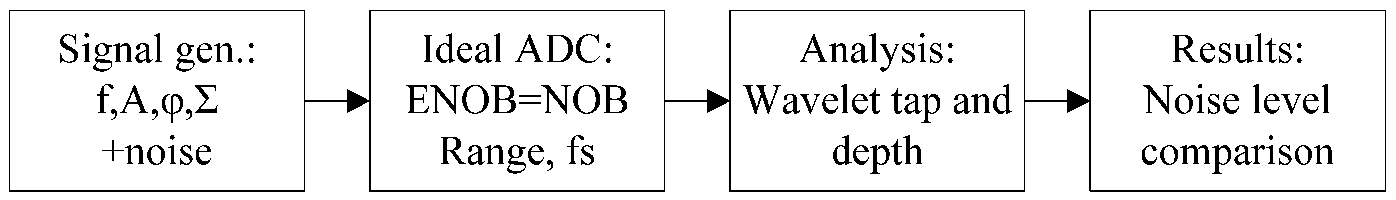
Power quality (PQ) measurements are based on separated measurements of voltages and currents. The characterization of measured data usually needs to happen in real time and results are depending on noise level. Today’s modern instruments need to be able to handle the signal variations and disturbance [1]. Also, the noise is mostly reactive component of power, and not taking the information of noise into consideration might mislead to the wrong measurement result. New signal processing algorithm can be used to improve the quality of measurement data. Today, even very complex algorithm can be calculated in real time, without data buffering, and this feature can drastically improve the quality of measurements results. Real time data analysis results in better controlling of system process, and drastically improving stability of systems. To evaluate the quality of energy there are many different approaches. Work presented in [2] deals with the problem of Perceived Power Quality determination in real time. Noise is not a steady process added to the signal, it is non-linear time variant process, so the noise reduction algorithm has to be robust but not aggressive on the signal. It has to be “smart”. Classical approach with static filters is not able to answer to all new needs in data analysis of PQ measurement data. Work [3] presents a real-time monitoring system for power quality, able to classify 20 disturbance classes, including multiple and single disturbances. Work presented in [4] deals with the calibration procedures of the measurement channel and the verification of the measurement characteristics and validation of the measurement algorithms. Reference [5] describes a new instrument for power quality (PQ) measurements based on an open-source hardware platform. This approach allows distributed PQ monitoring on a wide network and territory. In order to analyze the PQ it is necessary to measure the normed parameters using suitable instrumentation. Work presented in [6] provides a prototype of USB acquisition device capable to perform certified PQ measurements.

This paper proposes how to remove and reduce noise, but without changing the amplitude, the harmonic component nor phase of the measured signal. The noise reduction algorithms are often used to improve measurement characteristics and to determine parameters of analyzed systems. The wavelet transformation (WT) is widely used for image processing [7], analysis of non-electrical quantities [8], identification of system parameters [9], analysis of electrical power quality [10], GPS data analysis [11], noise smoothing for structural vibration test signals [12] and in many other scientific fields. The problem of optimization of wavelet threshold is addressed in [12], [13]. In the paper [14] the problem of disturbances’ detection is analyzed by using two different signal processing methods: wavelets and Hilbert Transform (HT). Both methods were tested under different conditions of noise and harmonic distortion (THD) showing the Hilbert Transform can be used as a valid approach for this type of phenomena.

In this analysis, the WT is used for noise reduction of power quality signals. The noise reduction is made with respect to dynamic ranges of power quality measurement setup. All generated signals are presented as percentage of Full Scale Range. In this way the results are applicable for both voltage and current measurement. Main problem is how to define noise reduction wavelet setup with respect to signal parameters to reduce noise, while not decreasing sensitivity to harmonics and events measurements. This paper is defining how to set and use WT for dynamical noise reduction with no a priori knowledge of noise distribution nor noise amplitude. Higher harmonics in signals with high level of noise are especially demanding for analysis and for reconstruction or extraction of data. This paper analyzed how to set the parameters of WT to be able to reconstruct important information from higher signal harmonics in PQ measurements.

In practice, the main problem is how to set thresholding levels, determine the level of decomposition and wavelet vanishing moment. In [15] three mother wavelet families are used: Daubechies (dbK), Coiflets (coifK), and Symlets (symK) up to levels 2 to 7. The best results are found for decomposition levels 5 and 6. In [16] Daub4 (4 vanishing moments) was used. In [17] authors used 10th level of decomposition and db5 (vanishing moments set to 5). In many existing manuscripts the vanishing moment numbers and decomposition levels used in denoising process are similar to our results presented in this paper, but they were set without exact analysis. The assumption is that usually authors made initial analysis by modifying these parameters and then they used the best parameters, or they selected some frame value. This is also the reasons why analysis presented in this paper are made: to find the best parameters (decomposition level and wavelet’s vanishing moments) of Perfect Reconstruction Quadrature Mirror Filters (PR-QMF) wavelet denoising according to closely analyzed simulated signals with perturbation without a priori knowing the standard deviation of noise.

2. Wavelet Filter Bank Decomposition and Signal Reconstruction

The main difficulty of analysis with Fast Fourier Transformation (FFT) is averaging of spectrum bins and phase shift. If the signal is divided into windows, then the result of FFT is convolution of signal and window spectrum, which in the end results in spectral leaking problem. The main contribution to spectral leaking problem is non-integer number of signal periods. Furthermore, signal filtering with FFT is resulting in phase shift, which needs to be compensated. These problems can be solved with WT.

The WT of signal x(t) is defined as [18]:

$$W\left(s,\tau \right)=\frac{1}{\sqrt{s}}{\displaystyle \int }\overline{\mathsf{\psi }}\left(\frac{t-\mathsf{\tau }}{s}\right) x\left(t\right)dt,$$

(1)

where s is scaling factor, usually set to 2, and τ is translation parameter of mother wavelet function ψ(t). Mother wavelet has the finite energy and mean value equal to zero.

Discrete Wavelet Transformation – DWT is defined as signal splitting into pieces with band-pass filter bank which is created by scaling the mother wavelet function [18]:

$${\mathsf{\psi }}_{\mathrm{j},\mathrm{k}}\left(t\right)=s^{\frac{-j}{2}}\mathsf{\psi }\left(s^{-j}t-k\tau \right), j,k\in \mathbb{Z}.$$

(2)

Practical formula (2) with s = 2 and τ = 1 is:

$${\mathsf{\psi }}_{\mathrm{j},\mathrm{k}}\left(t\right)=\frac{1}{\sqrt{2^j}}\mathsf{\psi }\left(\frac{t}{2^j}-k\right)$$

(3)

If the filters ψ _j,k(t) are orthogonal then every function x(t) can be written as:

$$x\left(t\right)={\displaystyle \sum }_j{\displaystyle \sum }_k{d}_{\mathrm{j},\mathrm{k}}{\mathsf{\psi }}_{\mathrm{j},\mathrm{k}}\left(t\right)$$

(4)

where discrete WT coefficients d are defined as:

$$d_{\mathrm{j},\mathrm{k}}= \langle x\left(t\right), {\mathsf{\psi }}_{\mathrm{j},\mathrm{k}}\left(t\right)\rangle =\frac{1}{\sqrt{2^j}}{\displaystyle \int }x\left(t\right)\mathsf{\psi }\left(2^{-j}t-k\right)dt.$$

(5)

To cover the full bandwidth from 0 to f_s/2 (f_s – sampling frequency) infinite number of wavelets need to be used. Therefore, the scale function is defined [19] (also known as Father Wavelet) which is impulse response of low pass filter. Scale function covers the bandwidth which is not covered by wavelet functions. Scale function ϕ(t) is also translated and dilated according to (3). Now on the R decomposition level the function x(t) can be written as:

$$x\left(t\right)={\displaystyle \sum }_{k=-\infty }^{\infty }{c}_{\mathrm{R},\mathrm{k}}{2}^{-\frac{R}{2}}\mathsf{\varphi }\left(2^{-R}t-k\right)+{\displaystyle \sum }_{j=1}^R{\displaystyle \sum }_{k=-\infty }^{\infty }{d}_{\mathrm{j},\mathrm{k}}{2}^{-\frac{j}{2}}\mathsf{\psi }\left(2^{-j}t-k\right),$$

(6)

where c_R,k are discrete scale coefficients. Scale and wavelet functions are made by inverse Fourier transformation of orthogonal FIR filters and their mirror functions, and they need to be Perfect Reconstruction Quadrature Mirror Filters (PR-QMF) [20]. In this analysis, the Daubechies wavelet family is used which is PR-QMF.

Vanishing moment (wavelet tap) defines up to which polynomial function degree some function can be analyzed by such defined wavelet and scale function. For Daubechies wavelet family the shorted inscription is dbX, where X is the number of vanishing moments. Therefore, db1 has one vanishing moment (can well describe discrete data in communication protocols), db2 has two vanishing moments (can well describe linear changes in signals) etc. Therefore, the WT needs to be adjusted to specific use and analyzed signals. The function with only one vanishing moment can describe only polynomial function of degree 0 i.e., the bias. This analysis defines decomposition level and number of vanishing moments which maximize the noise reduction in power quality measurement. For this task the Mallat’s DWT algorithm has been used [21]. Mallat’s DWT algorithm is adopted for numerical calculations in discrete domain. Signal is convoluted with high-pass and low-pass PR-QMF filters. The high-pass filter is de facto band-pass filter. Antialiasing filter wipe the upper part of signal spectrum above Nyquist frequency, the band-pass is covering remaining upper part of remaining spectrum and therefor it is named high-pass. Results from low-pass filtering is named approximation coefficients – a, and results from high-pass filtering is named detail coefficients – d. On the first depth of decomposition the result are Cauchy products [21]:

$$\begin{array}{c}{a}_1\left(n\right)={\displaystyle {\displaystyle \sum }_{k=-\infty }^{\infty }}x\left(k\right)g\left(n-k\right),\\ d_1\left(n\right)={\displaystyle {\displaystyle \sum }_{k=-\infty }^{\infty }}x\left(k\right)h\left(n-k\right).\end{array}$$

(7)

Coefficients g(k) and h(k) are respectively low-pass and high-pass filters impulse responses. Convolution between impulse response and analyzed signal will result with their spectrum multiplication. After first level of decomposition, the results are decimated by 2 (down-sampled). Decimation is removing every second element from approximation coefficients. Result is downsized number of data but also expanded frequency spectrum to the spectrum size of initial signal. In this way the same coefficient for low and high-pass filter can be used and algorithm is iterative and can be fast performed. New data length is:

$$N^{\prime }=\frac{N}{2}$$

(8)

where N is length of signal x(k) and N′ is new data length after decimation. Frequency resolution of x(k) and decimated data are:

$$\begin{array}{c}\Delta f=\frac{1}{N\Delta t}, \\ \Delta f^{\prime }=\frac{1}{N^{\prime }\Delta t}=\frac{2}{N\Delta t}=2\Delta f.\end{array}$$

(9)

Decimation is expanding the part of spectrum with important information to the original length. Now the next depth of decomposition can be calculated:

$$\begin{array}{c}{a}_2\left(n\right)={\displaystyle {\displaystyle \sum }_{k=-\infty }^{\infty }}{a}_{1\downarrow 2}\left(k\right)g\left(n-k\right),\\ d_2\left(n\right)={\displaystyle {\displaystyle \sum }_{k=-\infty }^{\infty }}{a}_{1\downarrow 2}\left(k\right)h\left(n-k\right).\end{array}$$

(10)

Symbol ↓2 is representing decimation with factor 2. This process of signal decomposition can be repeated until only one element remains after decimation. After the decomposition of signal, the threshold has been applied on coefficients [22]. Hard threshold is used because it preserves all edges which might be caused by flicker or voltage swallows and dips and does not smooth the remaining coefficient. The threshold level is fixed and set to universal threshold (square root log) [22]:

$$\lambda =\sqrt{2log\left(size\left(N\right)\right)},$$

(11)

where N is signal length. There are many different approaches for defining the threshold level, but without a priori knowledge of noise level, the threshold level is set to universal threshold. Main idea is to reduce the noise in signals without information about noise level. The threshold can change value corresponding to different levels of decomposition [23].

Hard thresholding $a_{\mathrm{HT}}$(n) of approximation coefficients a and d_HT(n) of detail coefficient d is defined as [24]:

$$\begin{gathered} a_{HT}\left(n\right)=\{\begin{array}{c}a\left(n\right) for \left|a\left(n\right)\right|>\lambda \\ 0 for \left|a\left(n\right)\right| \le \lambda \end{array} \\ {d}_{HT}\left(n\right)=\{\begin{array}{c}d\left(n\right) for \left|d\left(n\right)\right|>\lambda \\ 0 for \left|d\left(n\right)\right| \le \lambda \end{array} \end{gathered}$$

(12)

The wavelet coefficients with absolute value greater then threshold are preserved and other are set to zero. After thresholding, the signal is reconstructed with inverse filter banks which are PR-QMF and in this way the reconstruction is lossless.

Reconstruction of signal is also iterative process made by convolution of interpolated (up-sampled by factor two: ↑2) results from previous decomposition level and impulse response of inverse high-pass and low-pass filters used for decomposition process [21]:

$$\begin{array}{c}{a}_{a1}\left(n\right)={\displaystyle {\displaystyle \sum }_{k=-\infty }^{\infty }}{a}_{2\uparrow 2}\left(k\right)\tilde{g}\left(n-k\right),\\ a_{d1}\left(n\right)={\displaystyle {\displaystyle \sum }_{k=-\infty }^{\infty }}{d}_{2\uparrow 2}\left(k\right)\tilde{h}\left(n-k\right).\end{array}$$

(13)

The sum of these two data are new approximation coefficients on the level 1. Process is then repeated until the original starting signal length is not reached. Filters $\tilde{g}$ and $\tilde{h}$ are inverses of filters g and h. Reconstruction filters are orthonormal wavelets, and consequentially the sums of their spectrums are:

$$\begin{array}{c}{\left|H\left(\omega \right)\right|}^2+{\left|\tilde{H}\left(\omega \right)\right|}^2=1,\\ {\left|G\left(\omega \right)\right|}^2+{\left|\tilde{G}\left(\omega \right)\right|}^2=1,\end{array}$$

(14)

where G and H are frequency spectrums of filters g and h. The measure of noise reduction is represented with Peak Signal to Noise Ratio (PSNR). PSNR is defined as [25]:

$$PSNR=20lo{g}_{10}(\frac{2^{b-1}}{\sqrt{MSE}})$$

(15)

and mean squared error is defined as:

$$MSE=1/N{\displaystyle \sum }_{k=1}^N{\left(x\left(k\right)-x_{\mathrm{nr}}\left(k\right)\right)}^2$$

(16)

In (16) the original signal without noise is x(k) and signal with reduced noise is x_nr(k), N is signal length, b is number of bits.

3. Defining WT Parameters for Noise reduction

3.1. Introduction—Analysis Chain and Setup

If the measured signal is $x\left(k\right)$, signal with reduced noise is $x_{\mathrm{nr}}\left(k\right)$, the wavelet vanishing moment $d{b}_{level}$, the depth of decomposition is depth, then the main problem can be formulated:

$$max\{PSNR\left(x\left(k\right),x_{\mathrm{nr}}\left(k\right)\right) :inf\left(d{b}_{level}, depth\right)\}$$

(17)

The resulting parameters will result with maximal PSNR for infima, minimal, depth of decomposition and wavelet vanishing moment.

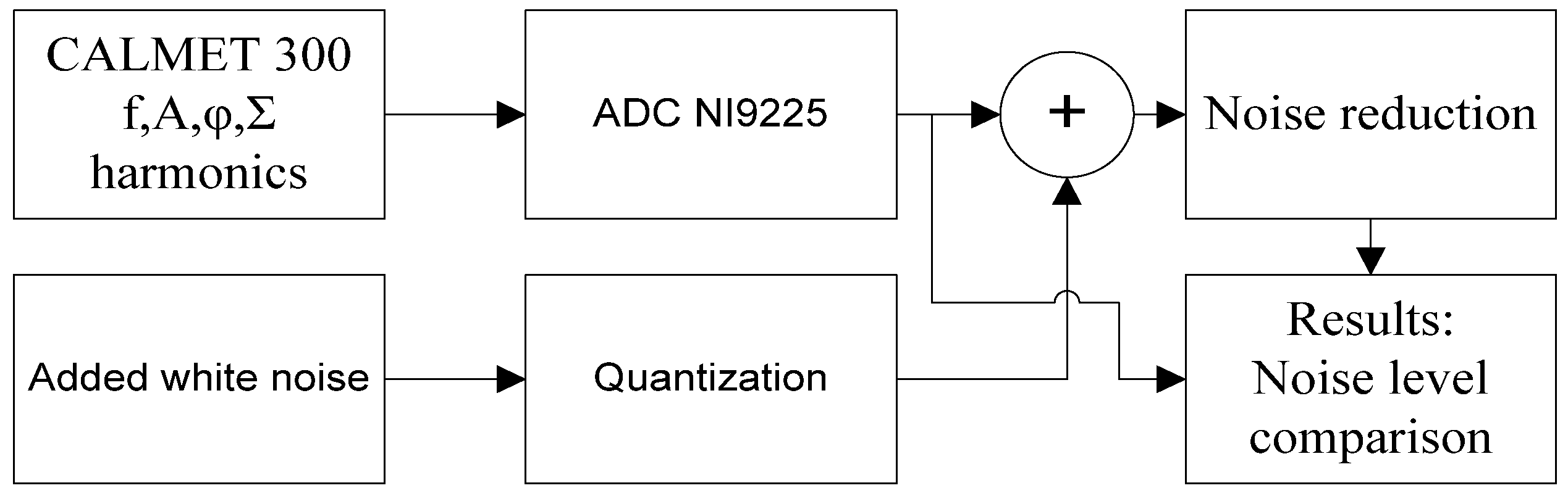
In this section the influence of wavelet decomposition parameters on quality of noise reduction will be analyzed. Input signal is simulated with corresponding amplitude, frequency, phase and other parameters. During the analysis the parameters of ideal 24 bit ADC, with full scale range equal to NI 9225 card are used.

Effective number of bits (ENOB) can be defined with Full Scale Range (FSR) and Noise and Distortion (NAD) parameters of ADC [26]:

$$ENOB={\log }_2\left(\frac{\frac{FSR}{G}}{NAD\sqrt{12} }\right)$$

(18)

where G stands for ADC’s gain. The parameter NAD can be defined in frequency domain [27]:

$$NAD=\frac{1}{\sqrt{N\left(N-3\right)}}\sqrt{{\displaystyle \sum }_{n\in S}{X}_{\mathrm{av}\mathrm{m}}{\left(f_n\right)}^2}.$$

(19)

In (19), $X_{\mathrm{av}\mathrm{m}}\left(f_{\mathrm{n}}\right)$ is the value of n_th spectral component on frequency n, averaged m times, and N is the number of elements of set S.

Sampling frequency is set to 50 kS/s (10³ samples per second). Time length of sample is set to 1 s. The discretized data are analyzed with different number of wavelet tap (vanishing moments) and depth of signal decomposition. Algorithm is also tested with different signal to noise (SNR) levels which are added to signal. SNR in decibels is defined as:

$$SNR=10\log \frac{P_{signal}}{P_{noise}},$$

(20)

where P stands for power. Analysis chain is shown in Figure 1.

This analysis generates huge amount of data, consequently the results will be presented in 3D graphs. In each analysis two parameters are variable and others are fixed. The parameters of efficient WT noise reduction are defined in the minimum number of analysis steps.

3.2. Simulation Analysis

3.2.1. Amplitude and Wavelet Vanishing Moments

Amplitude of generated signal is changing from 1 V up to 400 V. Frequency is set to nominal European power grid frequency of 50 Hz. Amplitude is presented as percentage of Full Scale Range (FSR). Signal to Noise Ratio (SNR) is set to 40 dB [26] of white noise. White noise is a noise with uniform probability density function (pdf), of which random variables are uncorrelated. Level of decomposition is set to 5, and vanishing moment (wavelet tap) is changing from Daubechies 1 tap (db1 is equal to Haar wavelet) up to Daubechies 7 tap (db7). Results are given as 8 bit PSNR in dB. This is presented in Figure 2.

As it can be seen from Figure 2, PSNR is coming to saturation for vanishing moment larger than 4, and for smaller values of amplitude the improvement is larger.

3.2.2. Amplitude and SNR

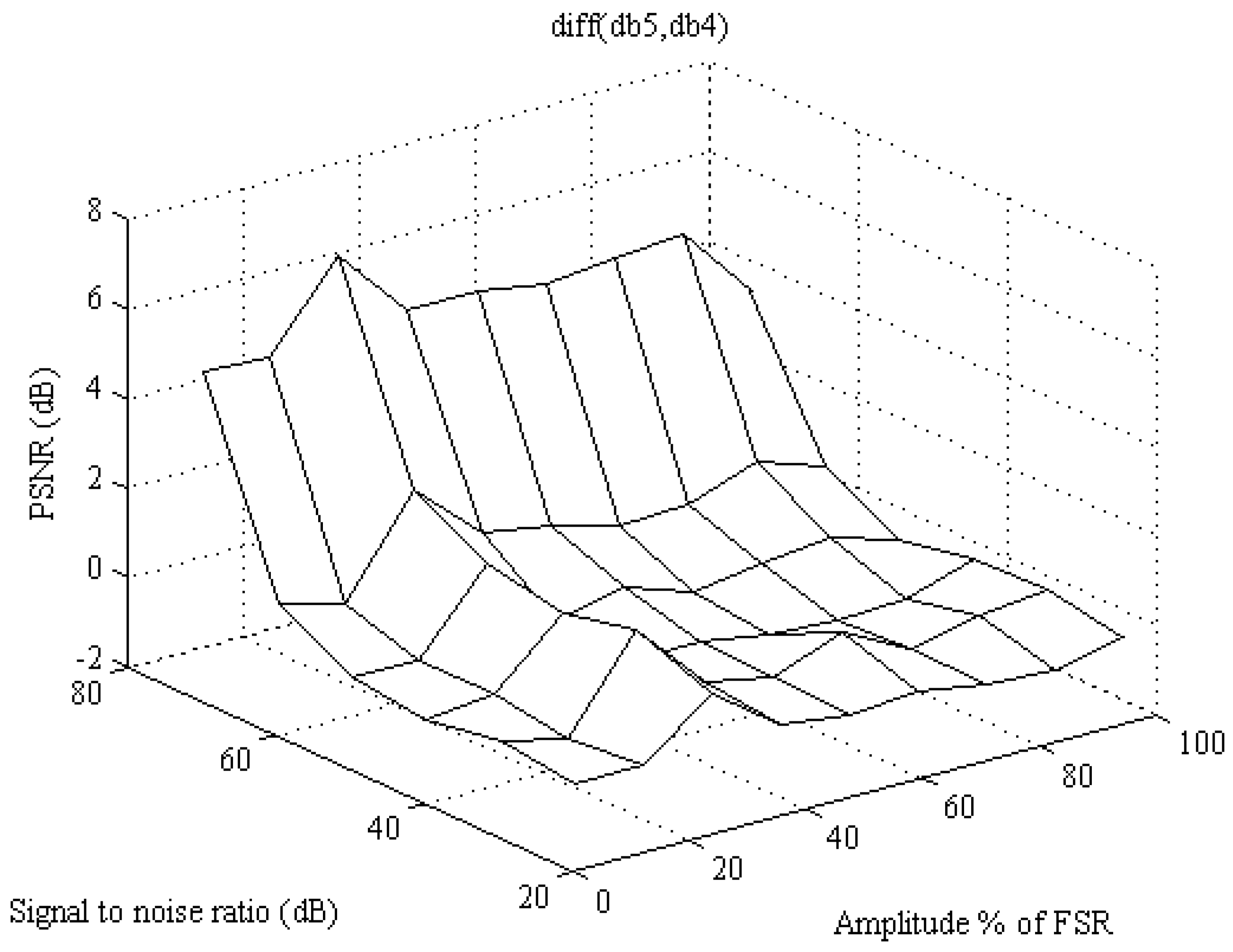
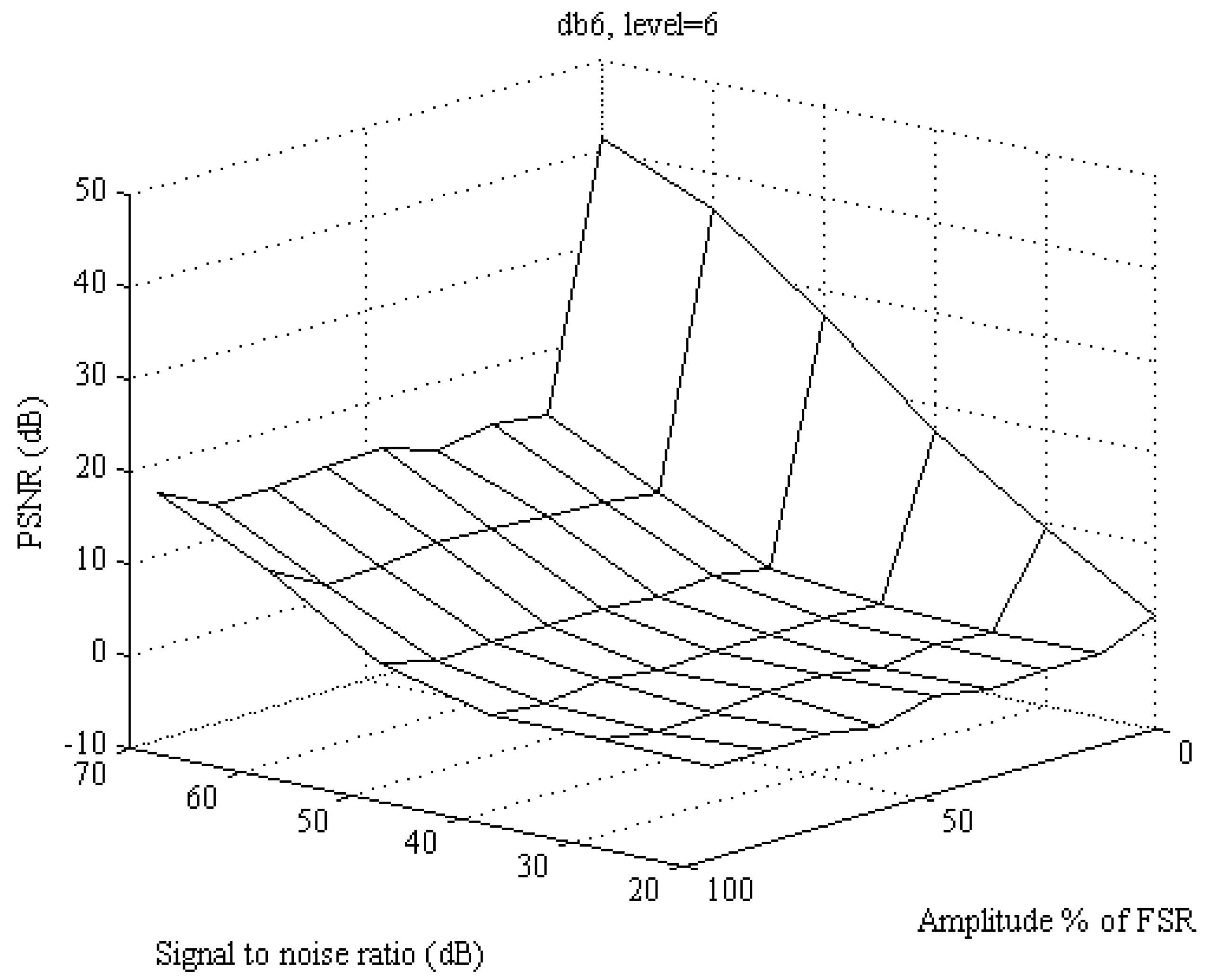
Amplitude is changing in range 1÷400 V, and it is presented as % of FSR. Frequency is 50 Hz, wavelet type is Daubechies, and level of decomposition is set to 5. SNR parameter is in range from 10 up to 70 dB. Aim of this analysis is to present the difference between the db4, db5 and db6. Figure 3 shows difference between db5 and db4 for different SNR and signal amplitude.

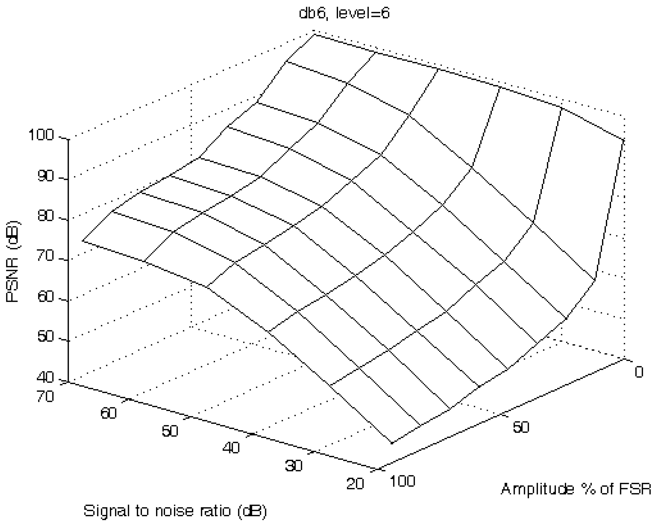
It is evident from Figure 3 that there is some difference and improvement between db5 and db4. The improvement is starting to rise for SNR higher than 50 dB. Further increase of vanishing moment is not producing any further improvement in PSNR. The difference between db6 and db5 is presented in Figure 4. The difference between db6 and db5 is negligible, resulting around zero and for 20% FSR amplitude the difference is negative. It is not contributory to increase the vanishing moment above db5. This analysis is made for decomposition level set to 5. Next, an analysis is made to check the ideal vanishing moment for different SNR and with nominal signal amplitude.

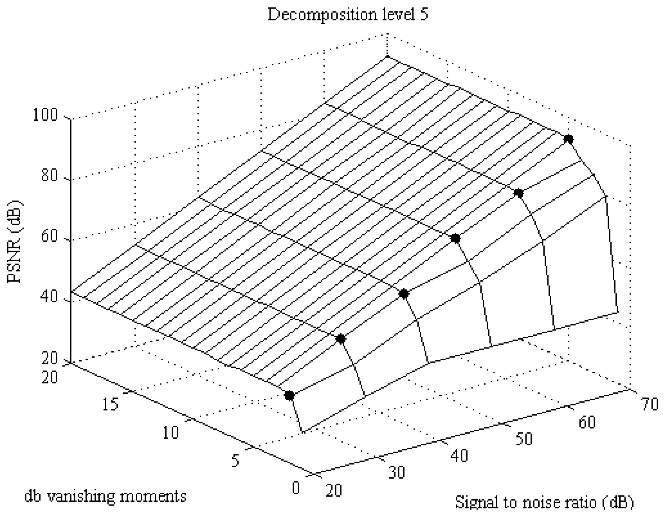
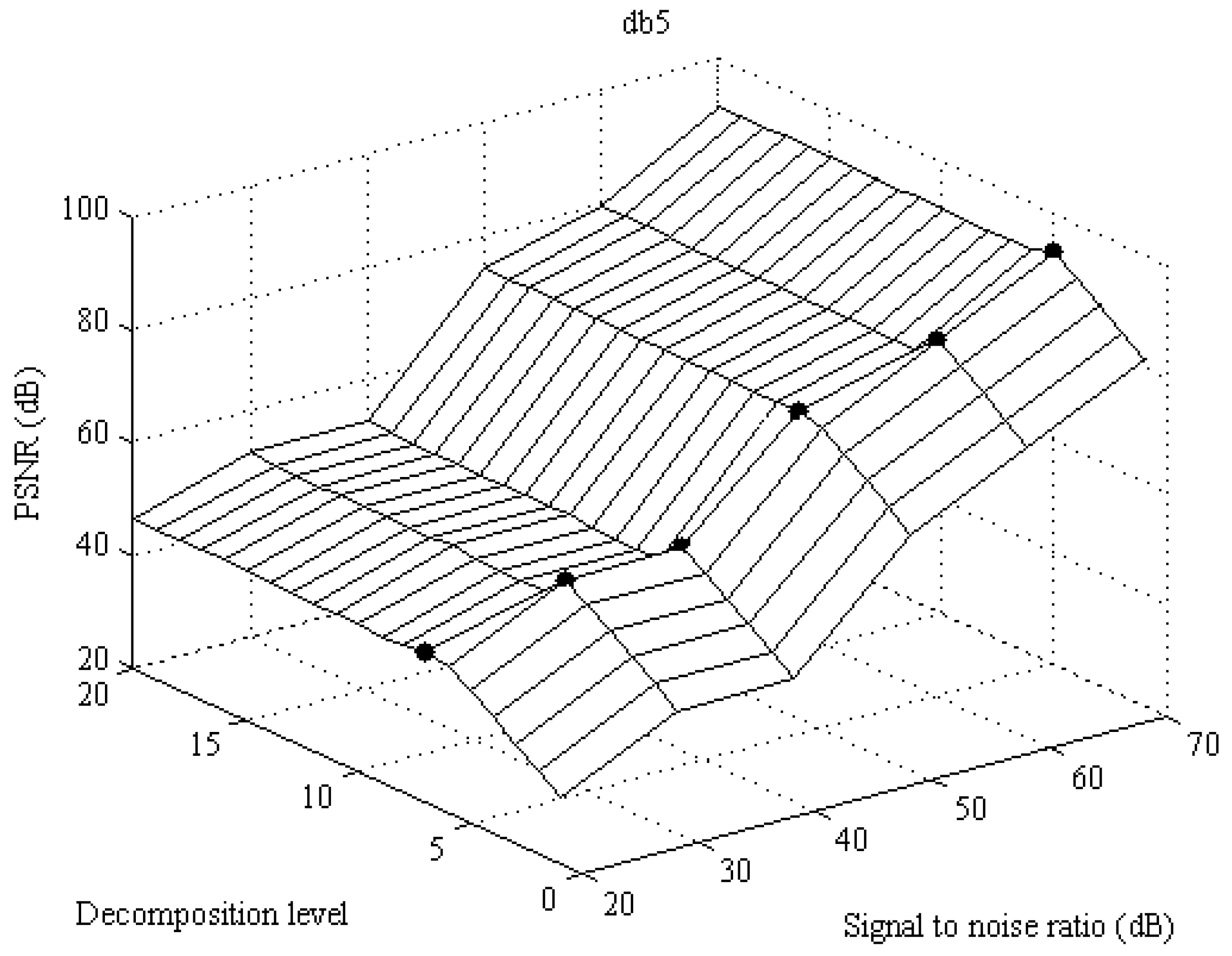
3.2.3. Vanishing Moments and SNR for 230 Vrms Voltage

In this subsection the influence of vanishing moments and SNR for 5th and 6th decomposition level on PSNR are analyzed. Amplitude of signal is set to 230 Vrms, frequency is 50 Hz and level of decomposition is 5. Vanishing moment is changing from 1 to 20 (step is 1) and SNR is changing from 20 to 70 dB with step equal to 10 dB. Main goal of this analysis is to determine which vanishing moment is satisfactory for which decomposition level. Results for 5th decomposition level are given in Figure 5.

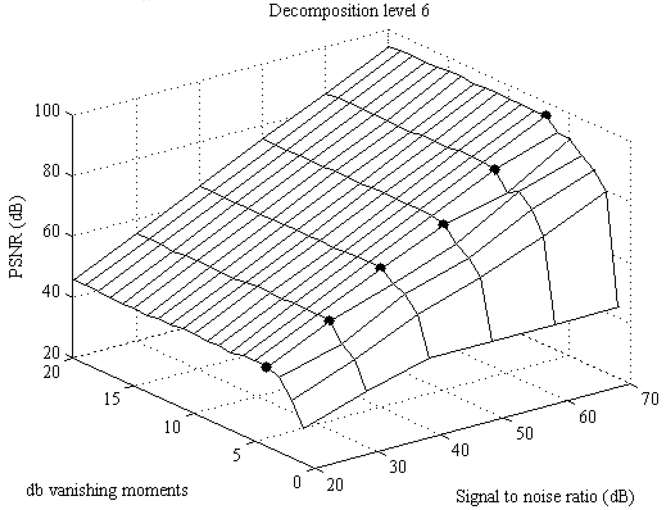
The points of reaching maximum are marked with black dots. For lower SNR the vanishing moment of reaching maximum PSNR is 2nd and it is increasing with SNR up to 5th vanishing moment. The results are similar for 6th decomposition level. Analysis is shown in Figure 6. For 6th decomposition level, the vanishing moments needed for reaching maximum are slightly increased compared to 5th decomposition level. For lower SNR the vanishing moment of reaching maximum PSNR is 4th and it is increasing with SNR up to 7th vanishing moment. If the 5th decomposition level is used, then there is no significant improvement by increasing vanishing moments above db5, and if the 6th decomposition level is used then there is no need to increase vanishing moment above db7. These results are made for nominal voltage with 230 Vrms, but in power quality measurement, dips, swells, overshoots and jittering is expected. For lower amplitude maximum is reached with lower vanishing moments and decomposition level.

3.2.4. Decomposition Level and SNR

Defining the optimal level of decomposition is demanding process. Many authors addressed this issue in their works [23,24]. This paper is trying to define the level of decomposition depending on saturation of PSNR. After defining the 5th and 6th vanishing moments as border values, they need to be tested for different decomposition levels to confirm the conclusions from previous subsection. Voltage is set to 230 Vrms, and frequency to 50 Hz. The first analysis is made for db5, and the second for db6. Level of decomposition is variable and it is changing from 1 to 20, with step equal to 1. SNR is changing from 20 to 70 dB with step equal to 10 dB. The result for db5 is presented in Figure 7.

For db5 the value of decomposition level in which the PSNR reached the maximum value is 7th for low SNR and 5th for higher values of SNR. Main conclusion is that for lower SNR it is necessary to increase either decomposition level or number of vanishing moment. Result for db6 is presented in Figure 8.

For db6 the maximum of PSNR is reached with 8th decomposition level for low SNR and 5th for 70 dB SNR. For lower values of SNR the results are very similar for 6th, 7th and 8th decomposition level. Main conclusion for this subsection is that there is no need to increase the decomposition level above 6th for both db5 and db6.

3.2.5. Harmonics Simulation Analysis

After defining wavelet decomposition level and vanishing moment the influence of denoising on signal harmonics was made. Test signal is composed of fundamental signal (230 Vrms @ 50 Hz) and 10 harmonics. Each harmonic has a different amplitude which is presented as percentage of 230 Vrms. Level of SNR has been changed from 20 to 70 dB. For each SNR the signal was denoised with Daubechies wavelet (level of decomposition is set to 6 and vanishing moment is set to db6). Amplitude of each harmonic was measured before and after denoising. Results of analysis are presented in

Table 1. Values of generated and measured signal harmonic as % of signal amplitude.

No. of Harmonics	3	5	7	11	13	17	19	27	31
	Generated harmonics (% of 230 Vrms)
Values	9.9991	8.9993	7.9987	6.9985	5.9976	4.9970	3.9958	2.9956	1.9955
SNR (dB)	Measured harmonics with noise reduction (% of 230 Vrms)
70	9.9991	8.9993	7.9987	6.9986	5.9976	4.9970	3.9958	2.9957	1.9956
60	9.9990	8.9995	7.9987	6.9985	5.9974	4.9969	3.9959	2.9958	1.9952
50	9.9995	8.9994	7.9983	6.9987	5.9983	4.9971	3.9954	2.9950	1.9933
40	10.0003	8.9982	7.9975	6.9964	5.9949	4.9928	3.9948	2.9969	1.9876
30	9.9947	9.0096	7.9893	6.9957	5.9886	4.9915	3.9827	2.9566	1.9858
20	10.0325	8.9988	7.9719	7.0432	5.8887	5.0188	3.9468	2.5968	1.4612

.

In Table 1 it can be seen that denoising algorithm presented in this manuscript is not attenuating any of signal harmonics components. Amplitudes of signal harmonics are preserved even for huge amounts of noise compared to their values. This analysis is verified in chapter 4. (Laboratory measurement and comparison of results) with signals generated from calibrator.

3.2.6. Interharmonics Simulation Analysis

For testing influence of denoising process on interharmonics the signals of interharmonics with various frequencies and amplitudes are added to the fundamental signal (230 Vrms @ 50Hz). Frequency of interharmonics goes up to 1 kHz. Level of SNR has been changed from 20 to 70 dB. For each SNR the signal was denoised with Daubechies wavelet (vanishing moment is set to db6 and level of decomposition is set to 6). Amplitude of each interharmonic was measured before and after denoising. Results of analysis are presented in

Table 2. Values of generated and measured signal interharmonic as % of signal amplitude.

Freq. (Hz) of Interharmonics	111	222	333	444	555	666	777	888	999
	Generated harmonics (% of 230 Vrms)
Values	9.9865	8.9712	7.9579	6.9487	5.9446	4.9459	3.9521	2.9625	1.9759
SNR (dB)	Measured harmonics with noise reduction (% of 230 Vrms)
70	9.9864	8.9712	7.9579	6.9487	5.9446	4.9459	3.9522	2.9625	1.9759
60	9.9865	8.9713	7.9577	6.9489	5.9447	4.9453	3.9522	2.9625	1.9759
50	9.9869	8.9711	7.9578	6.9496	5.9450	4.9460	3.9528	2.9625	1.9748
40	9.9890	8.9724	7.9575	6.9406	5.9460	4.9427	3.9542	2.9640	1.9715
30	9.9820	8.9717	7.9583	6.9695	5.9476	4.9423	3.9527	2.9618	1.8841
20	9.9753	8.9734	7.9516	6.9792	6.0004	4.8817	3.9214	2.8869	1.6398

.

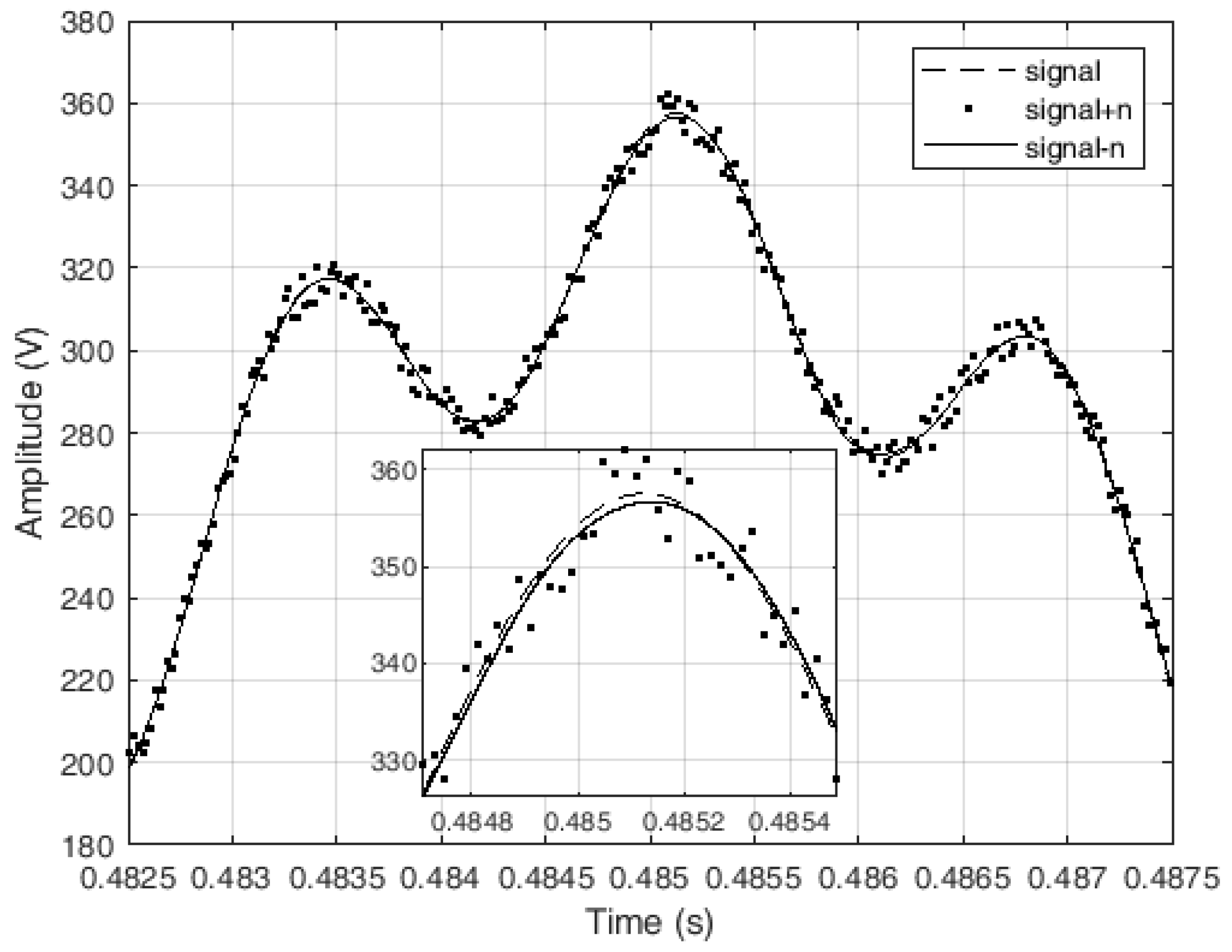
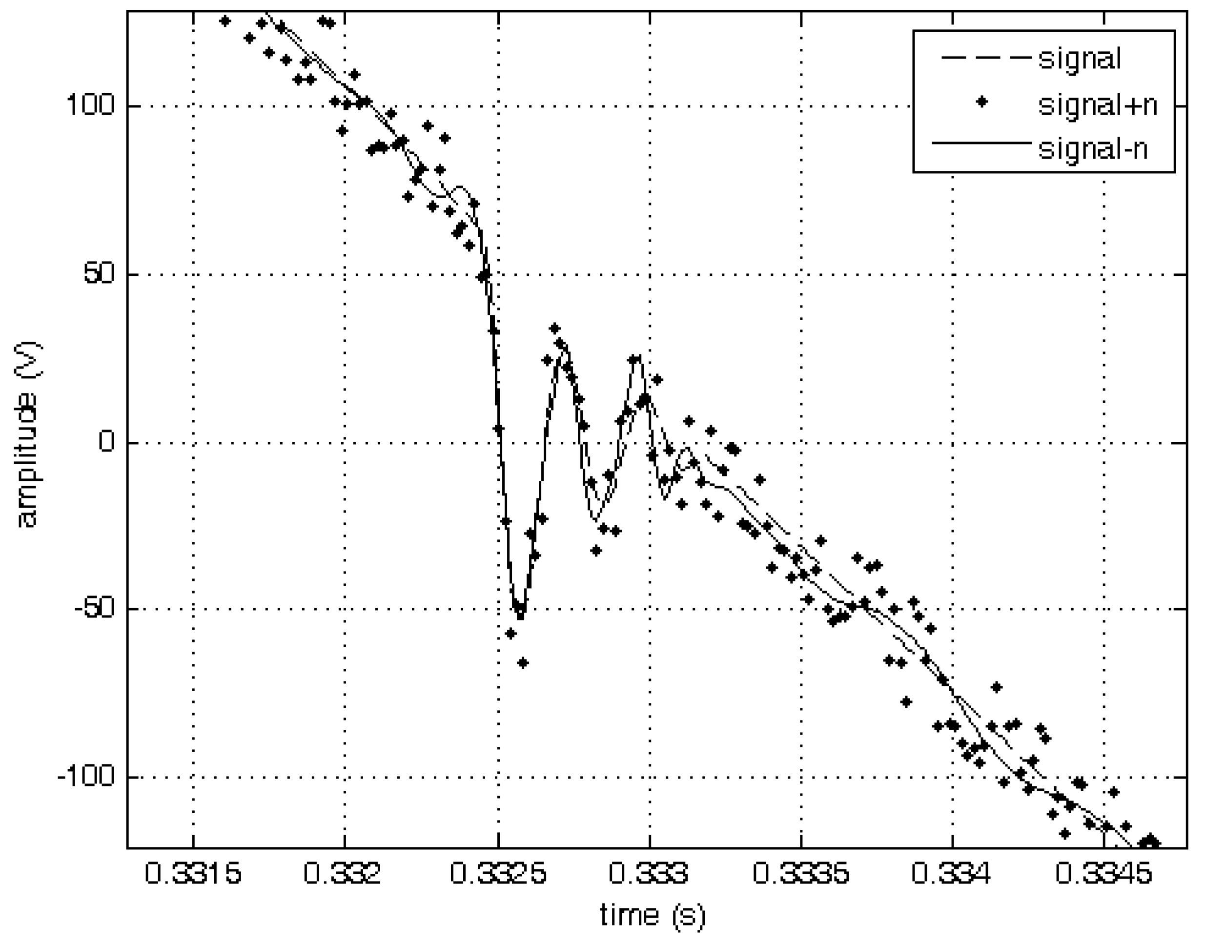
Analysis of signal with interharmonics presented in Table 2 shows similar results to previous analysis with harmonics. The algorithm for denoising is not attenuating amplitudes of interharmonics and they can be separated from signal and analyzed separately. Amplitudes of signal interharmonics are preserved even for huge amounts of noise compared to their values. Detail of signal with interharmonic with 555 Hz and 23 Vrms with 30 dB of white noise are presented in Figure 9.

Top part of positive period of signal with interharmonic with zoomed peak of signal has been shown in Figure 9. Denoising is made very precautious. Fundamental signal and interharmonic are preserved and energy of each of them can be additionally analyzed.

3.2.7. Transient and Interruption Simulation Analysis

Positive, negative and burst transient are added to test signal. Signal dip and swell are also added. According to EN 50160:2011 norm the dip is class A1 and swell is class cell S1 [28]. Interruptions are also added to signal. Vanishing moment is set to db6 and level of decomposition is set to 6. White noise is added in amount of 40 dB. One detail of test signal with positive, negative and oscillatory transient, swells, dips and interruption is presented in Figure 10.

Results of denoised signal presented in Figure 10 are presented with Figure 11.

Figure 11 is showing the error calculated by expression:

$$Error\left(i\right)=\frac{y_{dn}\left(i\right)-y\left(i\right)}{A_y} 100\%,$$

(21)

where $y_{dn}$ is denoised signal, $y$ is original signal with perturbations (without noise) and $A_y$ is nominal amplitude of fundamental harmonic which was set to 230 Vrms multiplied by square root of 2. Results of calculated error according to (20) is in range $\pm 1\%$. All information about dips, swells, transients and interruptions are preserved by wavelet denoising presented in this manuscript. Classification of dips and swells stayed unchanged after applying denoising algorithm.

3.3. Conclusions after Simulation Analysis

Algorithm presented in this manuscript is tested with various kinds of perturbation. For smaller values of amplitude, the improvement of denoising quality, indicated with amount of PSNR, is larger. Difference between db6 and db5 is presented in Figure 4 and it is negligible, and there is no significant improvement of PSNR values by increasing decomposition level above 6th. Suitable wavelet setup is to use db5 or db6 up to 6th level of decomposition. It will obtain good result both for dynamically changing amplitude of measured power grid signals and it is able to reduce noise for variating values of signal amplitude and SNR.

Algorithm can remove noise from signal without affecting the perturbation details of analyzed signal. Algorithm is showing good results with harmonics and interharmonics. Perturbation like transients, changes of signal amplitude and interruptions are also tested, and results are showing that denoising with wavelets is very sensitive to noise but it is not attenuating any of important parameters of signal.

4. Laboratory Measurement and Comparison of Results

4.1. Introduction—Measurement Setup

In this section the defined parameters after rigorous simulation analysis will be tested in laboratory measurement. Measurement setup is configured as presented in Figure 12. It consists of a Calmet C300—Three Phase Power Calibrator & Tester [29], NI9225 ADC [30] and program for noise reduction and noise level comparison.

Picture of measurement system is shown in Figure 13. On the left side is Calmet C300 with NI cRIO acquisition system connected on line voltages and currents sources. The screens are showing the software for generating signal, acquired data and algorithm for noise reduction according to solution produced by research presented in this paper.

The Calmet C300 is a class 0.05 three phase power calibrator and is used for signal generation. It can generate voltage up to 500 V with harmonics (up to 31st), and interharmonics. The C300 is also a three phase current source up to 100 A or one phase up to 300 A, and it is used as a power quality parameters generator. It is ideal for this type of measurement because the noise level comparison is made between the signal from ADC and the signal from noise reduction. With C300 calibrator it is possible to test various different parameters and algorithms for power quality measurements. NI 9225 is high quality 24 bits delta-sigma ADC with analog antialiasing filtering, 300 Vrms FSR and 3 simultaneous analog inputs with 50 kS/s frequency rate.

4.2. Amplitude and SNR Measurement Comparison

Generated voltage amplitude is in range 1÷400 V, and it is presented as % of FSR. Frequency is set to 50 Hz, wavelet type is db6 and level of decomposition is 6th. SNR parameter of noise is in range from 10 up to 70 dB. Result of noise reduction is presented in Figure 14.

For SNR greater than 50 dB the PSNR is in saturation, and there is no significant improvement with increasing SNR. Similar to the simulation, the best results are obtained for lower amplitudes. Figure 15 presents the difference between simulation and measurement results.

PSNR in Figure 15 is difference between the results from simulated signal from previous section and generated signal from the Calmet 300. The results show that there are no significant differences between simulation and real measurement for amplitudes from 10–00% FSR and for SNR levels 20–50 dB. In other areas the PSNR from simulation is higher for approximately 15–0 dB. For low amplitude and high SNR the simulation results are 15–0 dB better. This discrepancy is due to the Calmet 300 instruments’ class and the level of noise generated from it. For smaller amplitudes, the SNR is lower and this noise is superimposed to the one added in analysis. In this way the noise of instrument can be analyzed.

4.3. Harmonics and Interharmonics Measurement

As mentioned, the Calmet C300 system is able to generate signals with up to 31st harmonic. For this example the amplitudes of generated harmonics and measured results for different SNR are given in

Table 3. Values of generated and measured signal harmonic as % of signal amplitude.

No. of harmonics	3	5	7	11	14	17	19	27	31
	Generated harmonics (% of 230 Vrms)
Values	9.9771	9.0057	8.0153	7.0375	6.0521	5.0611	4.0597	3.0848	2.0719
SNR (dB)	Measured harmonics with noise reduction (% of 230 Vrms)
70	9.9771	9.0056	8.0153	7.0375	6.0521	5.0611	4.0597	3.0847	2.0718
60	9.9768	9.0055	8.0151	7.0376	6.0519	5.0611	4.0596	3.084	2.0718
50	9.9766	9.0062	8.0144	7.0371	6.0518	5.0607	4.0599	3.0843	2.0699
40	9.9782	9.0045	8.0165	7.0377	6.0527	5.0592	4.0565	3.0877	2.0668
30	9.9761	9.0076	8.0120	7.0433	6.0509	5.0637	4.0278	3.0743	2.0685
20	9.9676	8.9765	8.0280	7.0607	6.0179	4.9885	4.0380	2.7269	1.5039

. Signal amplitude is 230 Vrms.

Measured harmonics with different noise levels (Table 3) show that there is no influence of noise reduction to measurement results. Therefore WT noise reduction is fully capable to work with signals with many harmonics without interfering or attenuation. For SNR equal to 20 dB the result for 31st harmonic is lower due to large amount of noise. The energy of noise is overcoming the energy of harmonic. Noise is five times higher than amplitude of 31st harmonic.

For even higher levels of noise, the algorithm with parameters specified according to the analysis presented in this paper was able to remove noise and preserve the amplitude information of voltage. This is important for power measurement. All harmonics need to be taken into consideration when the power components are measured.

4.4. Voltage Burst

With Calmet C300 the voltage burst signal is generated and analyzed with added 20 dB of white noise, and the setup of noise reduction is the same as in previous subsection. One detail of burst signal is presented in Figure 16. This detail shows the fluctuation around zero amplitude.

Result of noise reduction is especially important in the sense of adding minimal phase shift. Even with a huge amount of added noise, the noise reduction is observable and cleaned signal is preserving the shape of original. With WT noise reduction, the huge amount of signal information in preserved, which is aim of noise reduction analysis. This setup of WT for noise reduction can be used in Phase Lock Loop (PLL) application. Due to the preserved original phase of signal, this algorithm is used in our laboratory for power and energy measurement in our ongoing Smart Grid Metrology (SMAGRIMET) project.

5. Conclusions

The systematic analysis made in this paper defines the wavelet transformation setup for noise reduction in power quality measurement. Main aim of this paper was to define depth of decomposition and number of wavelet’s vanishing moments for efficient noise reduction. The influence of signal amplitude, vanishing moment, decomposition level and SNR on quality of signal denoising are analyzed. After defining depth of decomposition and number of wavelet’s vanishing moments, they are used for denoising simulated signals with perturbations. Finally, defined parameters are used for denoising signals generated by three-phase calibrator. The results of this analysis are following: the decomposition level set to 6 and vanishing moment set to 6. These results prove to be a good option for signal denoising in power quality problems.

The process of defining the parameters of WT is very complex due to high number of parameters and huge number of simulations. Main contribution of this algorithm is in efficient noise reduction without prior knowledge of signal amplitude or SNR. The noise removal method remains sensitive to signal harmonics, interharmonics and amplitude deviation. The influence on the signal phase is negligible compared to the classic approach with filters so there is no need for phase correction. Wavelet noise reduction is powerful tool for dynamically changing signals in unknown environments in which the events are very important and need not to be defined as outliers.

Presented noise reduction setup is usable for both voltage and current measured data. Influence of WT noise reduction on power and energy measurement will be investigated in future work, due to large number of analysis and resulting data. Noise separated with this algorithm can be further analyzed. It is very important not to discharge noise data without knowing the source of produced noise. This algorithm, with parameters described according to this paper has been used for filtering data acquired with older equipment (lower precision and ENOB) in substations.