A Novel Control Architecture for Hybrid Power Plants to Provide Coordinated Frequency Reserves

Abstract

The inertia reduction suffered by worldwide power grids, along with the upcoming necessity of providing frequency regulation with renewable sources, motivates the present work. This paper focuses on developing a control architecture aimed to perform frequency regulation with renewable hybrid power plants comprised of a wind farm, solar photovoltaic, and a battery storage system. The proposed control architecture considers the latest regulations and recommendations published by ENTSO-E when implementing the first two stages of frequency control, namely the fast frequency response and the frequency containment reserve. Additionally, special attention is paid to the coordination among sub-plants inside the hybrid plant and also between different plants in the grid. The system’s performance is tested after the sudden disconnection of a large generation unit (N-1 contingency rules). Thus, the outcome of this study is a control strategy that enables a hybrid power plant to provide frequency support in a system with reduced inertia, a large share of renewable energy, and power electronics-interfaced generation. Finally, it is worth mentioning that the model has been developed in discrete time, using relevant sampling times according to industrial practice.

1. Introduction

During the last decades, penetration rates of renewable energy sources (RES) generation have steadily increased due to environmental concerns and positive market stances [1]. This trend is expected to continue during the following decades, partly motivated by international regulations [2,3]. In fact, some countries already present high shares of RES generation in their power systems, e.g., 43.4% of the Danish electricity consumption was covered by wind power in 2017 [4]. This renewable energy transition is positive and must be continued [3]. However, most of these generation units do not use traditional synchronous generators (SG), and thus are unable to provide inertia to the grid since all these units are not synchronously coupled with the grid. In addition, as RES-based generation increases, traditional power plants equipped with SG are gradually phased-out; ergo, new challenges arise in the power system, like loss of inertia, volatile frequency, and unwanted disconnection of distributed generation units [5].

In this context, even though frequency stability has, traditionally, been a simple task, nowadays it is becoming an increasingly complex activity due to the fluctuations of both generation and demand. European regulatory agencies, such as ENTSO-E, have already started giving the first guidelines and rules in order to ensure the correct operation of the electric system [6,7]. Such documents maintain the traditional structure with three stages of frequency control, acknowledging the fact that inertial response from SG is no longer sufficient, and opening the possibility to include smart control strategies in the new generation units in order to compensate such a lack. However, as will be presented in the next section, these new guidelines and rules are not yet clearly defined and stablished, as discussed in ref [8]. This new set of regulation not only has come to complete the normative of some countries were frequency control with wind power is not considered—like in Regelleistungand (association of German Transmission System Operators (TSOs)) [9]—but also modifies others like the most recent one from ENERGINET (Denmark), as will be presented in Section 7.1. [10]

On the other hand, industry has recently called attention to increasing the full load hours of wind farms (WF), which are defined according to the loading of the transformer in the plant. This value oscillates around 35% and 45% for onshore and offshore, respectively [11]. Briefly, if additional generation units are added to the system, the under-utilization of the plant will be reduced. 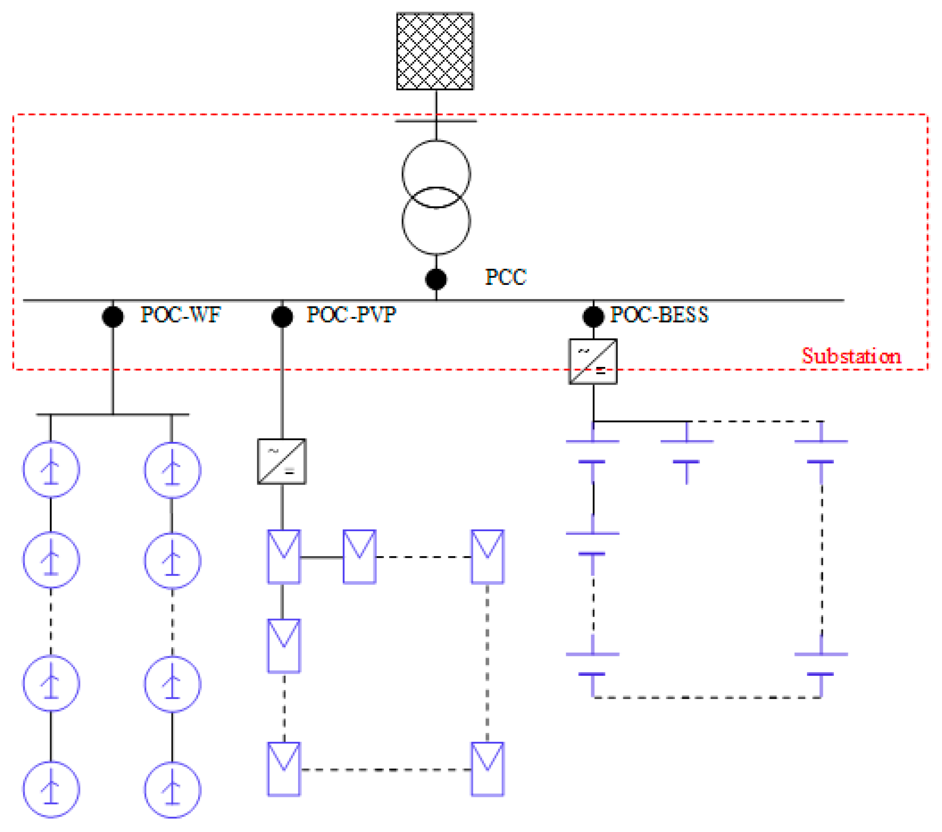Different manufacturers [12,13] are considering over-planting and the inclusion of a solar photovoltaic plant (PVP) in order to increase the production rate and complement it with a battery energy storage system (BESS). Such a plant will be capable of providing power smoothing, production loss minimization, and sudden power injections to help in the frequency regulation. Subsequently, a plant combining these three elements is referred to in this paper as a hybrid power plant (HyPP) and based on the benchmark model presented in ref [8].

Regarding frequency support with RES, there are barely any relevant works presented in academia, especially when considering HyPPs. In work such as refs [14,15], a combination of WF and PVP is used to provide an inertial response while others like refs [16,17] also include storage like flywheels. However, in all these studies, only the WF and the storage (if present) respond to the frequency excursion; none of them use a BESS, the model is always in continuous time (Laplace), and time delays accounting for event identification, measurements, or communications are dismissed. On the other hand, there are a few examples of site-tests made by industry, e.g., ref [18], a HyPP similar the one considered in this research that will finish its construction in 2019 in Australia. Then in refs [19,20], two combinations of WF and BESS in Denmark are also examples of how the Hybrid technology presents increasing interest to companies. However, the frequency control capabilities are still quite limited.

The main objective of this research is to evaluate the ability of HyPP to participate in the regulation of the system frequency by following current standards and system operation grid codes. Furthermore, a control strategy for the coordinated provision of frequency reserves in a system with a high share of RES and very low inertia is presented. In that respect, the model accounts for event identification and communication delays, and it uses current operational limitations of typical industrial controllers. It is expected that the HyPP’s combined response will be a sufficient and effective solution that is able to substitute conventional generating units due to the promising results presented in ref [8]. Although, in that work, only the first stage of frequency control was considered. Finally, it is worth mentioning that the proposed control algorithm including the hybrid power plant and external grid model has been developed for real-time hardware-in-the-loop (RT-HIL) studies. However, the results presented in this paper were obtained during the off-line verification stage according to the model-based design approach. The RT-HIL testing of the proposed control strategy is currently ongoing and will be presented in future publications.

The structure of the paper is as follows: A brief background review of frequency behavior is presented in Section 2, while current frequency regulation requirements and standards are covered in Section 3. Then, the system modelling, along with the HyPP concept, are covered in Section 4. Subsequently, in Section 5, the control architecture for the provision of reserves and its coordination is presented; whereas in Section 6, the design of every control stage is presented. Thereafter, in Section 7, the evaluation of the architecture and the model is addressed after defining relevant scenarios. Finally, the main conclusions of the study are stated in Section 8, and new research paths available for future work are highlighted.

2. Background in Frequency Behavior

Traditionally, Equation (1) has been used to define the simplified frequency behavior of any power system [21]. Such an equation expresses how a generation–demand imbalance causes a frequency variation, given that the speed or rate of that change is inversely proportional to the inertia and the size of the system:

$$ROCOF=\frac{P_G-P_L}{2HS}{f}_n$$

(1)

where ROCOF, P_G, P_L, H, S, and f_n stand for Rate of Change of Frequency [Hz/s or $\raisebox{1ex}{$ðf$}\!\left/ \!\raisebox{-1ex}{$ðt$}\right.$], total generated power [W], total consumed power [W], time constant related to the grid’s inertia [s], system’s total installed power [VA], and nominal frequency [Hz], respectively. ROCOF, which is defined as the time derivative of the frequency, has been historically dismissed in frequency control due to its low relevance in systems with high inertia. However, nowadays, due to the loss of such inertia, its use is becoming increasingly relevant. For the purposes of this study, the inertia constant has been set to 3 s, since it is a standard value presented by systems with high shares of RES, like Denmark [21].

3. Relevant Frequency Regulation Codes

The transmission system operator (TSO) is the agent in charge of ensuring the frequency stability of any network. At the European level, ENTSO-E elaborates and distributes a baseline of regulations to be followed by the countries belonging to such organizations. However, national standards can further develop regulations on top of those proposed by ENTSO-E. Nevertheless, recently, such regulations have been subjected to revision due to the changes experienced in power system behavior and operation resulting from the increasing RES and power electronic interfaces integration [6,7,22]. Subsequently, this paper uses up-to-date standards and regulations during the model development stage.

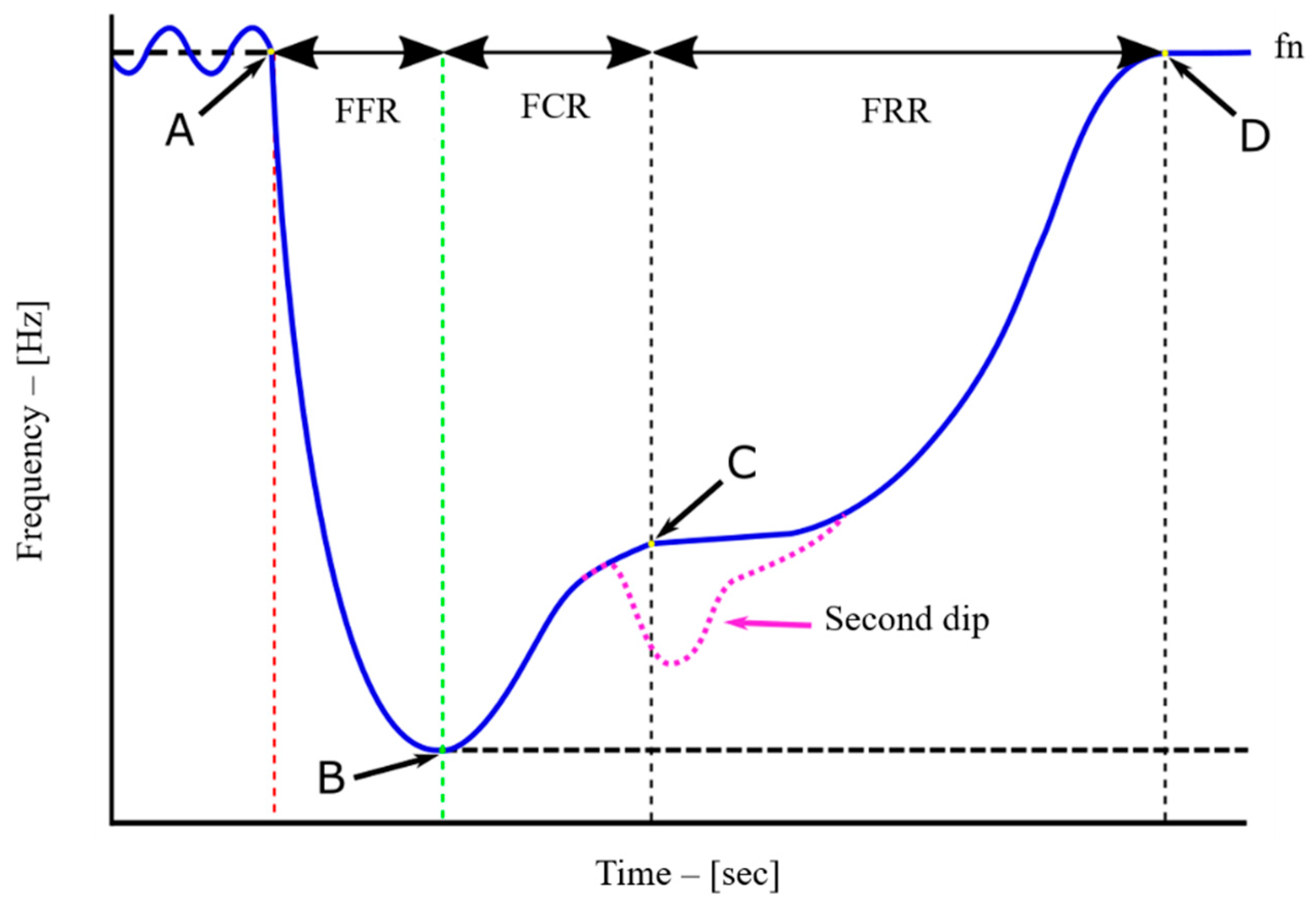
During steady state, the frequency oscillates in the vicinity of the nominal frequency value (50 ± 0.2 Hz); then; after the occurrence of an event, the nominal value is lost, and the three stages of frequency regulation start, namely: fast frequency response (FFR), frequency containment reserve (FCR), and frequency restoration reserve (FRR). Both the traditional and modern regulations acknowledge these three stages; however, there are certain differences and uncertainties that must be acknowledged. Additionally, the modern regulation opens the possibility of including a 4th stage called replacement reserves (RR). A typical frequency response to be expected after a down frequency event is presented in Figure 1. The pink line on the image illustrates the concept of a second dip, which is not yet covered in any regulation, but nevertheless, as will be explained, it represents a factor of major importance.

It should be mentioned how dips are caused by a generation vs. demand mismatch, which leads to discontinuities in the frequency recovery. In fact, systems with low inertia are especially vulnerable against such mismatches, which are usually caused by aggressive frequency response approaches.

3.1. First Stage: Inertial Response–Fast Frequency Response

This stage starts in the instant of the event detection and finalizes once the frequency reaches its minimum value. Such a point is known as ’Nadir’, with a corresponding frequency of f_nadir. Although there is no consensus regarding its duration, it is given mainly by the overall inertia present in the system, and thus it has a maximum from 2 to 5 s. It can be considered short, especially when compared with the other stages. As a reference, and due to the results presented in ref [8], it is considered to last from 0.5 to 2 s in this work.

The main difference between inertial response (IR) and FFR is that IR is provided exclusively by SG and in a natural, uncontrollably manner [12]. This means that, due to the physics ruling synchronism, SG naturally reacts in order to keep balance between generation and demand, and thus, stopping the frequency from changing. On the other hand, FFR is a controllable non-spontaneous reaction of the generators in a grid [12], which is, in short, a control-driven sudden power injection aiming to stop the frequency from continuing to modify its value. There are certain techniques to achieve this, like virtual synchronous machines, synthetic inertia, or the inclusion of spinning reserves [12].

In ref [7], FFR is acknowledged; however, there is neither a time length definition nor a specific approach to be followed in order to perform it. All the considerations taken regarding FFR in this paper are based on the work presented in ref [8].

3.2. Second Stage: Primary Frequency Regulation–Frequency Containment Reserve

This stage starts once the frequency stops dropping after the event (Nadir point); however, its end is not clearly defined in the regulations. In ref [7], it is simply stated that this stage finishes once the frequency has been partially restored, meaning that the frequency value is close to the nominal, but there is still an offset or error. The units participating in this stage are required to be able to provide full power injection during a certain period (around 30 min), although this time can be less if the third stage is activated prior to that. Again, there is no consensus regarding its time length; however, it is in the scale of several minutes [7,23,24].

The main differences between primary frequency regulation (PFR) and FCR is that PFR only considers the control action to be performed by the governors of different plants. Usually, PFR is performed only by one plant in the system in order to avoid the hunting effect. On the other hand, FCR is based on local frequency measurements. Basically, this stage is approached in both regulations as a droop control with a certain deadband in order to avoid over-actuation of the control system [7,23,24].

In ref [7], the procedure to be followed in order to estimate the FCR needs for a certain grid is stated. It also gives recommendations related to the droop characteristic and deadband to be implemented. Additionally, it states several time constraints: First, the FCR must start 3 to 5 s after the event is triggered and be fully activated in less than 30 s. Finally, it should be able to provide its maximum power capacity for at least 15 min. Lastly, the end of this stage is defined by this 15 min limitation or the activation of the third stage, whichever occurs first.

It is worth mentioning that the 15 min rule does not allow the renewable generation plants to participate in the regulatory market due to their dependency and uncertainty on meteorological conditions. However, the improvement of the short term meteorological forecast or the modification of this regulation might eliminate such limitations. Additionally, the inclusion of a storage system as in the case of the HyPP may already solve this challenge.

3.3. Third Stage: Secondary Frequency Response–Frequency Restoration Reserve

This stage starts after the second stage reaches steady state or after the time limitation; and finalizes once the frequency is restored to its nominal value or marginally close to it. Again, there is no consensus regarding its time length, but it is usually in the range of tens of minutes. It should be stated that this stage falls beyond the scope of this research, but it will be addressed in future publications.

There are no differences worth mentioning between secondary frequency response (SFR) and FRR as according to refs [7,23,24].

3.4. Fourth Stage: Tertiary Frequency Response–Replacement Reserves

This stage does not have clear start and ending points and, in both regulations, is considered to be optional. Thus, it is usually neglected in research. In the case of the tertiary frequency response (TFR), it consists of a set-point change in the conventional power plants based on an economic dispatch and unit commitment algorithms. While in the case of RR, it accounts for load variations occurring during the event clearance.

Again, this stage falls beyond the scope of this research, but will be addressed in future publications.

3.5. Final Considerations

The new regulations try to capture new technological realties present in power systems like the inclusion of renewable energy, inertia provision, etc. However, they seem like an ongoing work, especially due to the amount of amendments released during 2018 by ENTSO-E. Now, while these regulations are still being defined and established, is the moment to carefully analyze and review them.

In

Table 1. Summary of the frequency regulation processes.

Stage	Similar To	Main Objective
FFR	IR	Stop frequency variation
FCR	PFR	Approximate frequency to nominal value
FRR	SFR	Restore nominal frequency
RR	TFR	Final support

, a comparison of both terminologies is presented along with the main objective of each stage.

A second or subsequent dip is an additional frequency reduction that occurs during the restoration process, caused by a non-smooth recovery of the frequency. The frequency reduction of the second and subsequent dips is always of smaller amplitude than the Nadir. However, a grid’s stability is threatened even more, since frequency protections are triggered unnecessarily and thus will activate load-shedding schemes. The main reason for the protection to needlessly trigger is that first and successive dips are detected as a single fault with a comparatively long duration. Currently, most of the research regarding frequency restoration does not acknowledge the importance the second dip, as discussed in ref [8]. Although this second dip is not covered or defined in any standard yet, TSOs have raised their concerns in public talks (conferences, etc.).

4. System Modeling

In this section, the electric power system model is presented, including the description of the SG’s governors and loads included in the system. In a different subsection, the HyPP’s balance of plant is introduced.

4.1. Electric Power System

The considered grid—topology presented in Figure 2—represents an equivalent UK topology. It is based on the standard IEEE 12-bus system and adapted for wind power integration studies [25]. The system has four differentiated areas led by thermal power plants. Area 1 presents a large thermal power generation and a combination of residential and industrial loads. Meanwhile, rural loads dominate area 2, where there generation is also present. Subsequently, area 3 constitutes a heavily industrial load center with reduced thermal generation. Lastly, area 4 is the one marked in ref [25] as the connection point of wind farms for integration studies; thus, the HyPP is considered to be connected on Bus 5.

This network is suitable for the purposes of this research due to its simplicity caused by the fact of being an island and therefore avoiding the additional complexity of continental connections (limited size), which ultimately allows for easy implementation of frequency studies. However, the sizes of the conventional units have been altered in order to create a high HyPP penetration scenario.

Table 2. Summary of generation units’ sizes.

Generator	Size [MW]	Ratio [%]
SG: G01	750	21.75
SG: G02	640	18.56
SG: G03	384	11.14
SG: G04	474	13.75
HyPP	1200	34.8

summarizes the considered sizes.

The role of the SG is to represent the IR and primary frequency response as it is implemented nowadays. Those units respond to frequency deviations by means of governors, which are an extensively covered topic in literature [26,27]. It is worth mentioning that all the SG’s governors have been modeled as the F10 type (specifications can be found in ref [28]). On the other hand, the demand is aggregated and represents a mixture of different load characteristics, e.g., residential, rural, urban, industrial, agricultural, etc. Thus, half of this load is considered pure resistive loads while the rest are frequency dependent; that is, their active power demand is based on the grid’s frequency [26]. In order to account for those changes, all the loads are modeled as frequency-dependent, which is done by following Equation (2):

$$P_l=P_{lo}\left(1+D·\Delta f\right)$$

(2)

where P_l, P_lo, D, and Δf represent the total load, the non-frequency dependent part of the load, the load-damping constant, and the frequency deviation, respectively. In this work, D is assigned to be 1%, meaning that every 1% change in frequency would cause 1% change in the system load, whereas the standard value of the D constant is between 1% and 2% according to ref [29].

4.2. Hybrid Power Plant

As mentioned in Section 1, the HyPP concept is born from pursuing the idea of increasing the full production hours of WFs by adding additional turbines, a PVP, and a BESS. Thus, the included HyPP, which is based on the 100 MW benchmark model presented in ref [8], is compounded by three different sub-plants: WF, PVP, and BESS of sizes 100, 31.5, and 28 MW, respectively. The sizing, configuration and intra-plant loss estimation is extensively covered in ref [8]. However, it is important to note how the losses at nominal power and voltage in the PCC can be accounted for as a gain K_loss of 0.9921, 0.9658, and 1 for the WF, the PVP, and the BESS, respectively. This value was obtained in ref [8] after performing an extensive sensitivity analysis of the losses as a function of voltage level, active power, reactive power, short-circuit ratio, and R/X.

The balance of the plant is presented in Figure 3 where POC and PCC stand for point of connection and point of common coupling, respectively. It is assumed that in those points, there are measurement devices installed, i.e., grid meters. Lastly,

Table 3. Sizing of the HyPP in the benchmark model and in the implemented (scaled up) system.

Plant	Benchmark Size [MW]	Implemented Size [MW]
WF	100	1200
PVP	31.5	378
BESS	28	336
HyPP	100	1200

states the sizes of the HyPP both in the benchmark reference model and the implemented size in the tested scenarios of this research. As aforementioned, the benchmark model was 100 MW in ref [8]. Therefore, in this research, 12 of these plants are considered to be connected in Bus 5 of Figure 2, for a total implemented size of 1200 MW.

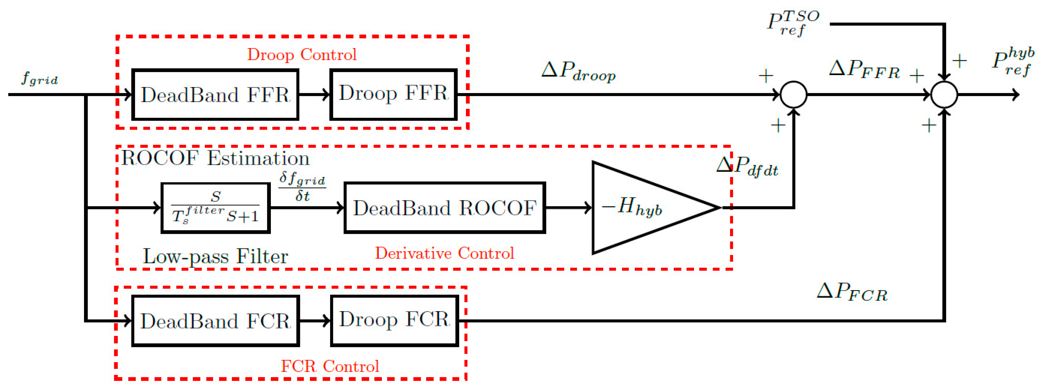
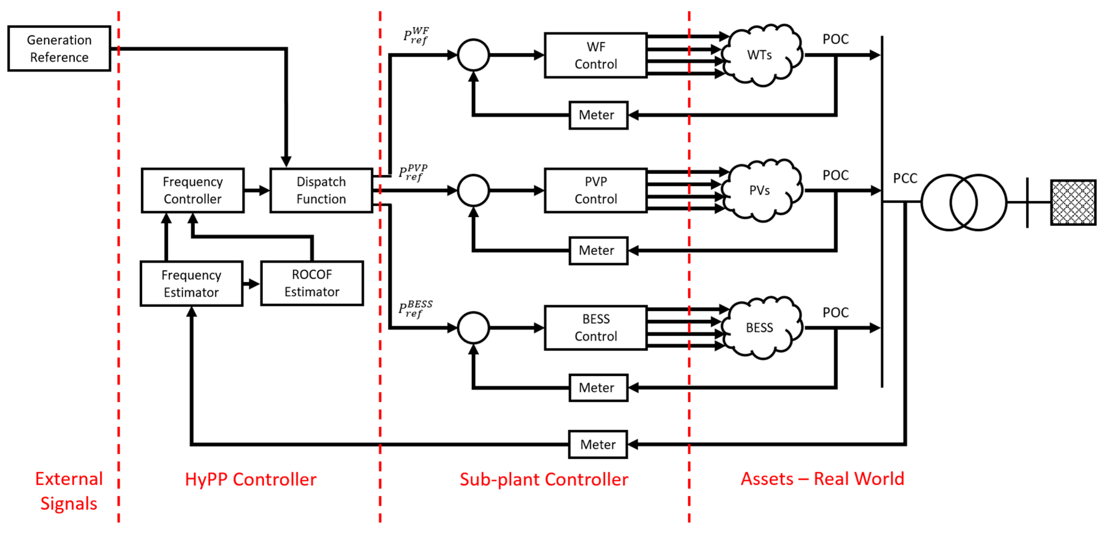
5. Control Architecture

In this section, a control architecture suitable to implement FFR, FCR with coordination of reserves is proposed. The objective of this approach is to allow the performance of frequency control while taking into consideration technical limitations like, capacity of commercial controllers, event identification and transmission of data (telecommunications).

The base line of this architecture is the proposed in [8] and it is presented in Figure 4.

The operational process is as follows; in normal operation, the TSO establishes a certain production set-point for the HyPP, which constitutes the generation reference. The Dispatch function will then divide the reference according to the available power of each sub-plant and to certain operational priorities (i.e., produce with the WF instead of discharging the BESS). Subsequently, each sub-plant controller will again perform a distribution of the reference among the individual assets (i.e., individual turbines). Then, after accounting for the internal losses by using a meter connected to the POC; the production of the three sub-plants is added, thus, obtaining the resulting performance in the PCC. The production of the HyPP is then fed into the grid as presented in Section 3.1. Then, by using the meter at the PCC, the frequency and, subsequently, ROCOF signals can be obtained. Both frequency and ROCOF, are fed back to the frequency controller; which will remain inactive until an event is detected.

According to the standards, an event is defined when the frequency falls beyond 50 ± 0.2 Hz, as defined in ref [7]. However, in the proposed method, an event can also be defined by a ROCOF value of ±0.2 Hz/s. In this way, the frequency contingency strategies are activated faster in case of a sudden event thanks to the ROCOF and also in low ROCOF events due to the frequency. Additionally, the over-activation of the frequency control is still avoided.

After an event is detected, a flag is raised, thus altering the dispatch’s operation and starting the frequency controller. Briefly, this controller uses frequency and ROCOF inputs to modify the operational set-point of the HyPP, thus coordinating the different frequency recovery stages. Regarding the operation of the Dispatch after the event is detected, FFR starts, with the objective to slow down the frequency excursion by combining the three sub-plants and dividing the effort as much as possible in order to provide a fast and harmless response. Then, FCR starts once the Nadir is reached, a point where ROCOF is 0. It should be stated that, according to the standards, FCR actions should start as soon as possible and in less than 2 s after the event identification, and thus being added on top of FFR as traditionally was with IR and PFR [7]. Subsequently, the HyPP combines the three sub-plants in order to approximate the frequency to its nominal value. Then, the BESS alone will perform the FCR actions since it is easier to control and it can act fast, avoiding behaviors that might threaten the frequency recovery or the plant’s lifetime (e.g., over-oscillations, vibrations, etc.). Since it is also possible to know the available energy and power available in the BESS from its state-of-charge, the minimum time of operation can be ensured. On the other hand, in the power system block, the SG reacts uncontrollably to the frequency excursion with IR and then PFR, in accordance with the standards.

In order to estimate the available power of the HyPP at PCC, power requirements from the grid–P_ref and external parameters influencing sub-plant production—wind speed, temperature, irradiance—are considered. Power requirements from the grid are based on requirements established from the system operator (SO) and those related to frequency regulation and the provision of FFR and FCR. On the sub-plant level, the input is a reference power from the control structure comprising of a ‘Dispatch’ block, which coordinates the different sub-plants. The output of each sub-plant is based on the input reference power requirement, external parameters, and unit dynamics. The overall output of the HyPP is then fed into the PCC.

6. Control Design

In this section, the design of the frequency controllers is addressed, starting with the evaluation criteria and continuing with each control stage implemented in the HyPP. It is worth mentioning that the developed model has been built by following industrial standards and common practices in order to resemble a real system, i.e., including sampling times for various blocks and subsystems, communication delays, etc. Therefore, even though the controllers were first designed in continuous time (Laplace), they were discretized using backward Euler due to its simplicity [30] and usefulness [8].

6.1. Success Criteria (Objectives)

The minimum performance requirements are established by different grid codes, regulations, and technical limitations of the involved elements [6,7,23]:

• Sub-plant’s settling time must be less than 10 s for a 0.1 p.u. variation.
• Sub-plant’s steady state error must be less than 2% without overshoot.
• Frequency must not drop below 49.2 Hz, a point were load-shedding protocols are activated.
• After FCR activation, frequency should be recovered to a value closer to the nominal than to the Nadir.

6.2. Plant Controllers

The selected controllers are PI, which were designed by replacing the slowest pole of the sub-plant’s transfer function with a pole in the origin. This approach yields a closed loop transfer function with a response similar to the sub-plant. Equation (3) presents the transfer function of the controller where G_PI, K_PI, T_PI, and s stand for the controller’s transfer function, gain, time constant [s], and the Laplace operator respectively:

$$G_{PI}=K_{PI} \frac{T_{PI}s+1}{T_{PI} s}$$

(3)

T_PI has the same value as the sub-plant’s time constant, while K_PI is obtained as presented in Equation (4), where K_Loss represents the intra-plant losses as presented in Section 4.2. Finally,

Table 4. Implemented PI-controller parameters [8].

KPIWF	TPIWF [s]	KPIPVP	TPIPVP [s]	KPIBESS	TPIBESS [s]
1.008	1	0.3106	0.3	0.005	0.005

presents the values of the implemented PI controllers’ parameters.

$$K_{PI}=\frac{T_{PI}}{K_{Loss}}$$

(4)

The Root locus and Bode plot of the closed loop of every plant after the addition of a PI controller were analyzed in order to study the gain range within stable operation. Figure 5 presents both diagrams for the WF’s controller where G_ol, G_cl, and PI stand for open-loop, closed-loop, and controller’s plants. However, a detail design for PV and BESS sub-plants as well as more details can be found in ref [8]. It can be seen how the system is stable for any gain, and the gain margin is also infinite, since the phase never crosses 180° and the phase margin corresponds to 89.1°, resulting in a stable system as was expected from the root locus. Subsequently, Figure 6 presents the step response of the WF, where the signals corresponding to the reference, the controller, and the plant behavior are shown.

6.3. FFR Controller

Due to the non-existence of consensus regarding the topology of FFR. However, as explained in [8], droop and derivative (df/dt) control have been used for years in automatic frequency control. Thus, a combination of them has been implemented; being the main novelties implementing it in a HyPP, use discrete modelling and real-time testing. Both control stages act in a similar way, once the deadband is cleared they apply a constant gain, which will be positive or negative depending on the event, to the reference signal; frequency for the droop and ROCOF for the derivative. The composition of the FFR controller is presented in Figure 7, while a summary of the implemented parameters is shown in

Table 5. Implemented PI-controller parameters.

Parameter	Unit	Value	Notes
Deadband Droop	Hz	0.5	Reduce activity of the control
Droop Constant	%	5	Slope of the Droop control
Deadband df/dt	Hz/s	0.2	Reduce activity of the control
TLPF	s	0.025	Low-pass filter’s time constant
HHyPP	-	5	Gain of the derivative control

[8].

6.4. FCR Controller

In Figure 7, the FCR control is also present. It should be stated that there is no strict rule regarding the appropriate droop constant to be implemented, although ref [7] recommends values between 2% and 12%, whereas it states that values between 3 and 5 are implemented in practice. Thus, during the FCR stage, a value of 5% was chosen.

7. Case Study

The selected scenarios evaluate the HyPP’s participation in frequency control. As aforementioned, the considered system presents a low inertia due to its high RES penetration. The considered event is a N-1 Contingency, which is defined in ref [7] as the loss of a single generation unit or a transmission component. In this case, SG G02 is tripped, causing a sudden considerable generation loss. After the event is detected, the system reacts to it, first by stopping the frequency drop and, subsequently, bringing it back to stable values close to the nominal. These are the purposes of FFR and FCR, respectively. The system is also considered to be in a steady state with a nominal frequency during the initialization, and the demand does not change throughout the simulation. Although, due to the frequency dependency of part of the load, as explained in Section 4.1, its effective value will change according to the frequency value. Therefore, the only variations are related to the active power production of the plants, which is caused by the frequency controller and demand due to their correlation with frequency.

Table 6. Steady-state operative points.

Unit Name	Steady-State Power Output [MW]	Steady-State Share in Total Generation [%]	Steady-State Power Output [%]
HyPP	600	40.0	50.0
G01	300	20.0	40.0
G02	200	13.3	31.3
G03	100	6.7	26.0
G04	300	20.0	63.3

presents the steady-state operative point of the system, and it should be noted how the last column refers to the operational point of the plant related to its size, which can be checked in Table 3.

7.1. Scenario Definition

The selected scenarios represent the same system, event, and response strategy, but a different detection and deadband. In Scenario I, ENTSO-E grid codes are fully complied with, which means that the event is detected when the frequency drops below 49.8 Hz, and the controller starts to act once its value is 49.5 Hz. In Scenario II, the event is detected either when the frequency or ROCOF fall below 49.8 Hz or −0.2 Hz/s, respectively, and the controller starts acting immediately after the detection. However, in both scenarios, the rest of the system is kept unaltered.

Table 7. Differences between Scenarios.

Difference	Scenario I	Scenario II
Event Detection	50 ± 0.2 Hz	Frequency ∉ $\left(50\pm 0.2 \mathrm{Hz}\right)$ ROCOF ∉ $\left(\pm 0.2 \mathrm{Hz}/\mathrm{s}\right)$
Frequency Deadband	50 ± 0.5 Hz	none
ROCOF Deadband	none	±0.2 Hz/s

shows the major differences between the considered scenarios.

It should be mentioned that a deadband for the frequency controllers was necessary in traditional power systems with high inertia, since the uncontrollable synchronous response will dampen and correct all the small excursions. In this way, over-actuation of the controllers was avoided. However, in modern, low inertia systems, this deadband is not useful anymore, since due to the low inertia, the response of the system will be extremely limited. That, combined with higher levels of ROCOF, makes it crucial to act fast. In the past, the frequency response was only activated after large excursions; however, in future scenarios with virtually no inertia, FFR has to be activated continuously in order to counteract small imbalances in generation and demand as the traditional IR does. Subsequently, in Scenario II, no deadband is set for the frequency in order to smoothly compensate with the FFR while the ROCOF deadband accounts for the identification of major excursions. Due to lack of scientific literature covering the topic, the value of ±0.2 Hz/s has been obtained after studying the response of the system during normal operation and after events triggered. Values up to ±0.1 Hz/s could be found if small load variations were inserted for the load, and thus the selected value provides a wide error margin, which is sufficient for the purposes of this research.

The objective pursued with these two scenarios is to highlight the importance of reviewing the recommendations provided by ENTSO-E in ref [7].

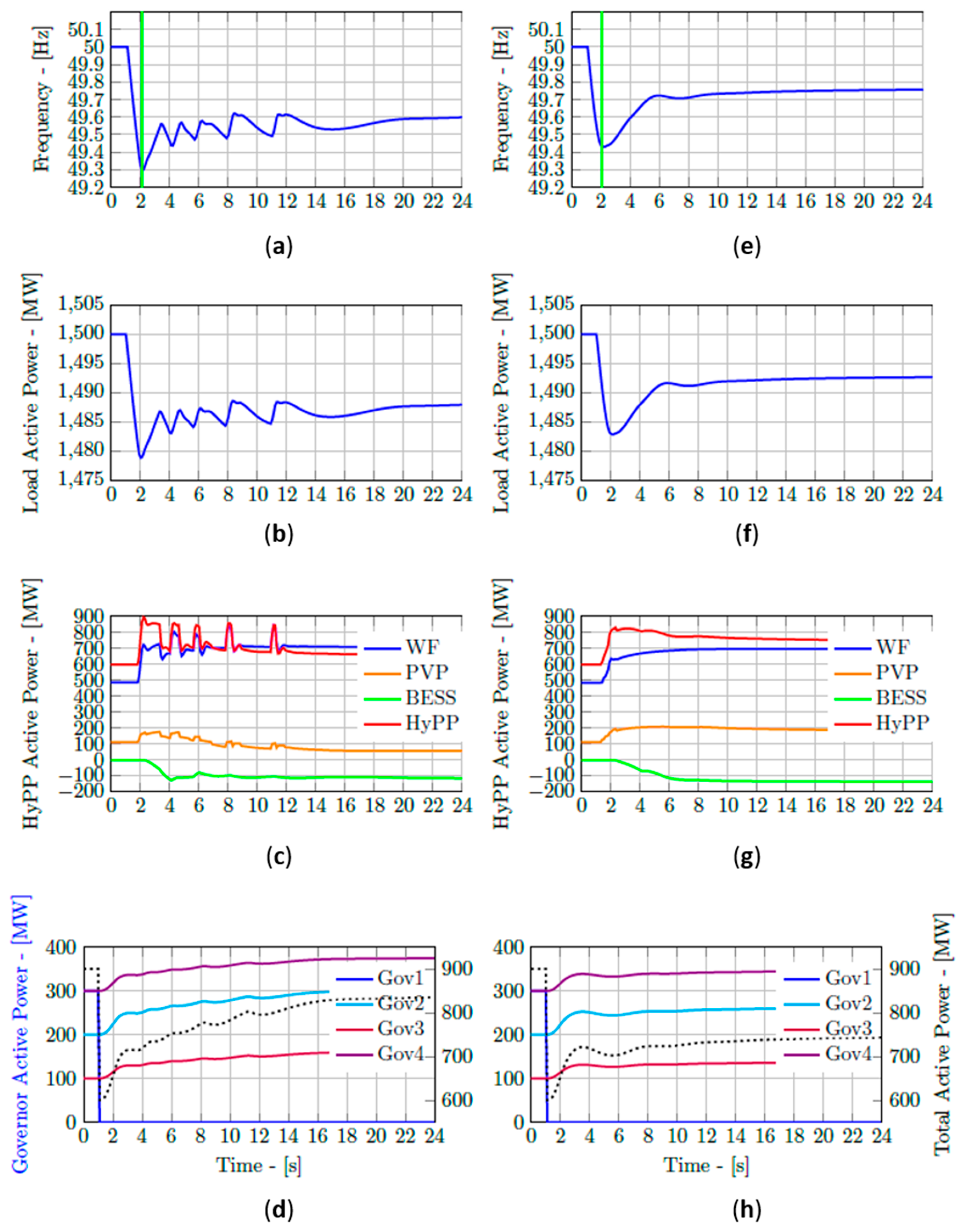
7.2. Tests Results

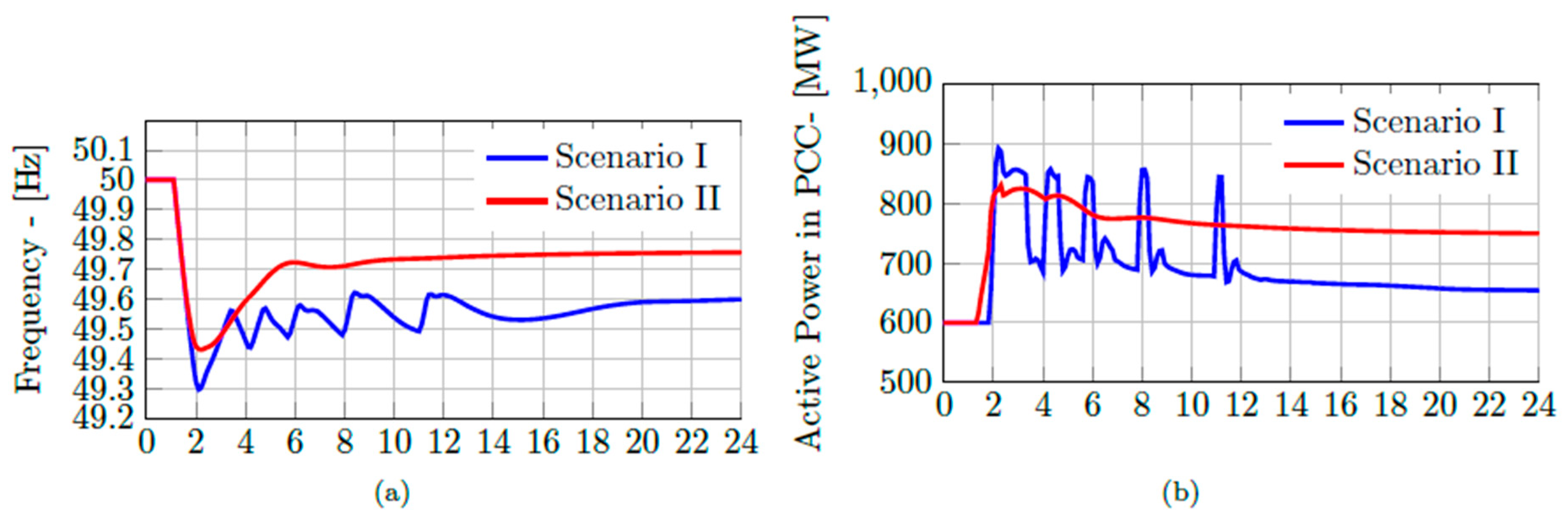
In Figure 8, the results of both Scenarios I and II are presented in different columns. The frequency response of the system is presented in Figure 8a,e where the Nadir is highlighted with a vertical green line. Subsequently, in Figure 8b,f, the active power demand of the system is presented and has a shape is similar to the frequency due to the dependency presented in Section 4.1. Thereafter, the generation provided by the HyPP is presented in Figure 8c,g, which is divided into each sub-plants’ actuation as well as the overall result. It should be noted how negative values of production in the BESS case represent a charging process. Finally, Figure 8d,h present the actuation of the governors, in which the disconnection of Gov2 is clearly shown. Note, how in these pictures, the legend of the left axis, which corresponds to the signals from individual governors, is only present in Figure 8d while the right axis legend, which corresponds to the overall response from the governors, is only present in Figure 8h.

In both scenarios, the SG and HyPP react to the N-1 contingency—ones based on a natural phenomenon and others by applying a control approach after the event is identified and the deadbands surpassed. It should be stated that the event identification time delay is accounted for along with the discrete actuation of modern controllers.

7.3. Discussion

In Figure 8, is clear that the change in the reference signal and deadband level improves the behavior of the whole system’s response. A comparative of the frequency behavior is presented in

Table 8. Overview of the simulation results.

Parameter	Case I	Case II
Nadir frequency [Hz]	49.29	49.43
Nadir time [s]	1.1	1.2
Frequency steady-state [Hz]	49.61	49.76
Time to reach steady-state [s]	27	20

, where the Nadir is shown to be reached faster but at a lower frequency for Case I. This is because the HyPP starts reacting after the frequency drops below 49.5 Hz, while in Case II, it does this immediately after the detection of the event, which is, again, faster due to using ROCOF. Thus, the reaction can be smoother. Additionally, the steady-state value reached by the FCR reaches stability faster in Scenario II, but the frequency value is also closer to the nominal. Furthermore, when comparing the dynamic responses in Figure 8c–g, it can be seen that the stresses suffered by the HyPP are reduced in Scenario II. This is important, since wind turbine manufacturers are concerned about the mechanical stresses suffered by WF providing frequency support. The PVP is also almost completely curtailed in Scenario I, while it increases its production in the second scenario, making the system more efficient. Finally, in Figure 8d–h, the response of the governors is also smoothed out and reduced. Finally, Figure 9 has been included in order to highlight the most important differences between both scenarios. Figure 9a presents how, in Scenario II, the frequency response is not only smoother but also recovers values closer to the nominal after the event, while in Figure 9b, the active power response in the PCC highlights how the power is also injected in a smoother manner into the power system, which improves the overall response of the grid and thus avoiding over-oscillations.

8. Sensitivity Analysis

Since all the work has been developed as a simulation, it is important to assess the influence of modifying different parameters on their behavior. In

Table 9. Parameter summary of the sensitivity analysis.

Parameter	Values		Notes
	Original Scenarios	Tested
H	3 s	2 s 5 s	The inertia constant of the grid depends of the size of the synchronous units connected to it
FCR delay	3 s	1 s 5 s	This value corresponds to the time delay in the activation of the FCR stage after reaching the Nadir. Ref [7] specifies that it should start in less than 3 s.

, a summary of the parameters subjected to the sensitivity analysis can be found. It is worth mentioning how all the studies have been conducted on top of Scenario II.

The results of this analysis are presented in Figure 10, where it can be seen how reducing and increasing the delay for FCR actuation improves and worsens the system’s response, respectively. Similar behavior also occurs after the modification of H, where larger parameters imply a higher stability of the grid, and thus higher stiffness.

9. Conclusions

In this paper, the importance of frequency provision has been addressed along with the causes that lead to inertia loss in worldwide grids. Subsequently, the relevant background related to frequency behavior has been introduced and associated to current regulations and recommendations from ENTSO-E, with focus on ongoing and questionable components. Since those regulations are still in the development stage, it is a matter of utter importance to assess whether they are targeting appropriate objectives with the correct methods. This is exactly the aim of this research—to evaluate if there are open paths for improving the frequency behavior, taking into account possibilities that so far appear to be dismissed by regulating agencies.

In Section 4, the system modeling is briefly presented, since most of it is extensively described in ref [8]. Thereafter, Section 5 presented the proposed architecture of the system, while the design of the different control stages was covered in Section 6. Then, in Section 7, two different scenarios were defined, both studying the same event—an N-1 contingency—but with a different event detection approach. Scenario I implements a frequency monitoring detection technique, as ENTSO-E recommends, with a considerably large deadband for the controller, while in Scenario II, ROCOF is the signal triggering the activation of the frequency controller. Consequently, the results show how the frequency behavior of the system is greatly improved. Even though the Nadir is reached later in the proposed method, the frequency reached is 8.5% higher, and the steady state error improved by 61.53 % in Scenario II. Additionally, the dynamic response of the generators in the system is smoother in Scenario II, satisfying one of the greatest concerns for wind turbine manufacturers: mechanical stresses and premature aging due to frequency support provisions. Finally, Section 8 presented a brief sensitivity analysis on top of Scenario II, pointing out the effects of modifying model parameters such as H.

The impact of the proposed architecture is the speed in event identification. The sooner an event is detected as a fault, the sooner the plant will react. On the other hand, some oscillations are always present in any system working within normal operation, which makes the objective of the existent deadbands to reduce over-actuation. However, the value of the nominal frequency has traditionally been used as a deadband. This paper proposes the use of ROCOF in event identification, since it allows the identification of fast excursions (like the ones appearing after an N-1 contingency) before the frequency can reduce its value and thus easing the system necessary reactions. Finally, it is worth mentioning that since the model has been developed for RT-HIL studies, future publications will cover the testing of this model in such frameworks, including industrial controllers for HyPPs.