1. Introduction
As an electricity supply source, wind power is one of the most popular options for avoiding greenhouse gas emission products from fossil fuel combustion, which has a major impact on global warming. This renewable energy source is currently a competitive solution in the electric market. Proof of its efficiency includes the global cumulative installed capacity of 539,123 MW [
1] at the end of 2016 and the competitive costs around the world [
2]. For example, the average levelized cost of energy in the USA in 2015 was 44 USD/MWh [
3].
Electric production using wind turbines has versatile applications, the most popular being the wind farm. However, this is not the only means by which wind can be used to supply electricity. The application of small wind turbines (SWTs) for the decentralized use of energy [
4] is a popular option for isolated grids, rural residential electrification, and hybrid systems [
5].
Furthermore, wind energy in urban environments is an open opportunity in several areas: renewable electrical generation, ventilation, pollution dispersion, and mitigation of the urban heat-island effect. Although technical issues must be solved to reach technological maturity, the literature includes examples in which the electricity generated could satisfy around 5–40% of the local demand using vertical-axis wind turbines (VAWTs) [
6].
In recent years, SWT applications have become a popular option for satisfying in situ demand. In 2014, the worldwide installed capacity was 830,332 kW, distributed among China, the USA, and the UK, which together represent 86% of the sector [
5]. On average, the power of each installed SWT in 2014 was 0.87 kW, and the main applications are oriented toward satisfying off-grid demands. Initial costs in the US range from 6840 USD/kW, corresponding to a wind turbine with a nominal power of less than 2.5 kW, to 4710 USD/kW, with a power range of 11–100 kW [
7].
Around the world, small wind energy is moving toward becoming a competitive alternative to power distributed generation. Two factors influence its development: policies to promote the technology and the costs of the systems [
8]. In this contribution, we study the resource assessment stage for SWT applications in an urban environment. The importance of resource assessment cannot be understated; its results and reliability (1) determine the development of the project, (2) are the basis of the techno-economical analysis, and (3) enable the development of economic scenarios that promote social penetration of these technologies.
Resource assessment is one of the most critical stages of any renewable energy project. Electricity production using wind power is calculated from wind speeds. Therefore, data quality is a crucial factor in power estimation. A complete review of the methodologies for resource assessment is presented in [
9], and the research on urban wind energy is reviewed in [
10]. For large wind turbines, the 10-min mean time has been considered to be a reliable method for power estimation and is widely reported in the literature. However, for small wind turbine applications, a reliable resource assessment is still a work in progress.
The literature includes studies aiming to determine the feasibility of implementing SWTs in urban environments throughout the world. In Greater London, the United Kingdom, the ideal regions for SWT electric generation were studied [
11], and in Guelph, Ontario, Canada [
12], it was estimated that SWTs could potentially supply 10% of the electric demand. In southern Italy [
13], the techno-economic potential of this technology was analyzed, and in the Edinburgh Region [
14], the wind speed potential from a meteorological database was found to be represented by a Weibull statistical model. The results of this study indicated that 72% of the time, wind speed was greater than 3 m/s, which is suitable for micro wind turbines. In the Gaza Region, a study analyzed the power produced by a 5 kW wind turbine, which was installable on the roof of a residential building, and the results indicated an annual capacity factor of 6%; further, wind power production may be complemented by solar panels to improve power performance and to provide grid stability [
15]. In this contribution, we present a technical analysis to describe the regional wind speed, and we assess different SWT models. This work is complemented by economic aspects that considering the Mexican electric context.
The power performance of an SWT is susceptible to wind resource availability. For example, local wind speed variability and high wind speeds that are available due to the building’s altitude result in wind power integration being an attractive alternative to decentralized power generation [
16,
17]. Therefore, an accurate description of the wind conditions in these complex locations is crucial [
18].
Urban environments are zones characterized by higher turbulence conditions that contain higher amounts of energy [
19]. Recent work has shown evidence of an increase in SWT power production due to the energy contained in gusts [
20]. This energy has effects on the output of a resource assessment analysis; there is a demonstrated relationship between the mean time of the wind speed used and the energy estimated [
21]. Therefore, a proper characterization of wind conditions at the location of interest will improve the reliability of assessments for this technology.
An additional factor that can improve the reliability of the power resource assessment for SWT projects is the inclusion of a dynamic description of the device in the analysis. Reliable calculations require the selection of a proper mean time for the wind speed time series used to feed the model. In this way, it is possible to include the energy contained in the gusts in the assessment, and it may improve power estimations [
22].
Although the reliability of the resource assessment can be improved by using wind speed data measured with specific characteristics and including specialized dynamic models, the development of the analysis becomes unfeasible for a domestic user. In this work, an adjustment to the methodology for estimating small wind turbine production is proposed: the proposed approach includes using data available from meteorological stations and calculating the differences in energy assessed according to time series averaged at different times.
The result of a resource assessment analysis is the calculated annual energy production of the selected SWT. The standard methodology for determining economic viability is to estimate the costs related to installation, operation, and maintenance. The latter factors are commonly associated with the lifetime of the technology. A cash flow model represents all components. Then, the relation between the energy produced and the costs of the project can be obtained. The levelized cost of energy can be calculated and complemented by other economic criteria, such as the time of investment return, cost–benefit analysis, etc. There are several examples of the use of this methodology that can be consulted [
23,
24,
25,
26,
27].
Nevertheless, these parameters may not provide precise information to a potential domestic user of the technology in Mexico due to electric regulations. Thus, this methodology is adapted to describe the Mexican electrical tariff context where can be implemented these technologies for distributed generation. The model includes the perspective of the domestic user and allows to compare wind turbines with different lifetime. The objective is to provide a methodology that contributes to analyzing and delimiting economic strategies to promote the use of this renewable source of energy in this specific sector.
2. Wind Power Sector in Mexico
Geographically, the wind power potential in Mexico can be divided into five regions: the Isthmus of Tehuantepec, the State of Baja California, the Gulf of Mexico coast, the Coast of Yucatan, and the Northern-Central region [
28]. Wind power resource assessment in Mexico has been studied in several works in the literature using different methodologies.
The Isthmus of Tehuantepec presents the most significant wind power potential in the country. This was the first zone studied for wind power generation [
29]; nowadays, nearly 60% of the total installed capacity in the country is concentrated in this region [
30]. A meteorological mesoscale model was used in the analysis, with a squared resolution of 2 km validated with 20 meteorological stations.
In Baja California, wind speed has great potential to participate in the transmission, distribution, and supply of electric energy to small urban zones [
31]. The southern region of this state is characterized by geographic complexity and presents a technical challenge to electric grid integration; therefore, wind power has become a viable option for electric supply [
32].
Veracruz and Tamaulipas are two states located on the coast of the Gulf of Mexico. In Veracruz, a wind persistence analysis was presented to study wind conditions for power production. Five meteorological stations were used with a mean time of 1 h. The results indicated that wind conditions were suitable for wind power production [
33]. A second study for the same state utilized seven meteorological stations and one anemometric tower to implement a statistical analysis of wind power potential in the region; the results agreed with those of the previous work [
34].
In the coastal zone of Tamaulipas, a resource assessment analysis was developed; the methodology consisted of comparing four anemometric stations with the BMW-CERSAT reanalysis. Then, wind power potential was modeled using the Wind Atlas Analysis and Application Program (WAsP). Although the power density results differed from those of previous work, the Tamaulipas coast remains a promising renewable source of electricity generation along the coast. However, it was recommended to have high-quality wind data for different locations and altitudes to better estimate wind resources [
35].
In northern Mexico, wind power was assessed using 237 different meteorological stations within Sonora, Chihuahua, Coahuila, Nuevo León, and Tamaulipas. To map the average monthly wind speeds in these states, an interpolation was implemented using the Kriging method. The analysis indicated that Tamaulipas is the state with the highest power density, and Nuevo León presents a large part of its territory with a power density of more than 230 W/m
[
36].
In the Yucatan Peninsula, Gulf of Mexico, wind speed distribution is bimodal at lower heights. Researchers studying this region compared the results from the Weather Research and Forecasting Model (WRF) with measured data, and they concluded that mesoscale simulations may serve as a preliminary wind resource for a coastal region with low-lying areas [
37].
The above-mentioned review offers several insights, including Mexico’s opportunity to use wind energy for electricity generation, the importance of resource assessment analysis, and the diversity of methodologies for estimating power production. However, according to the literature, there have been no studies implemented in Mexico that present a techno-economic analysis of wind power technologies for either large or domestic applications. Also, a common issue among the works presented is the lack of reliable data sets available to use in the validation of resource assessment analyses.
In Mexico, regulatory actions have been implemented by its government through the so-called “Energetic Reform” since 2013, and the objectives include strengthening the energy sector, improving costs, attracting investment, and protecting the environment by promoting the use of clean energy sources, such as renewables, for electric generation. In particular, wind power plays a vital role due to wind potential. The potential installed capacity has been estimated to be 158,000 MW for a conservative scenario that includes high potential zones and a distance from the transmission grid of less than 10 km [
38,
39].
Figure 1 presents the evolution of the wind power capacity installed over the years, as well as a projection for 2030. For the development of the wind power sector, defined goals for 2020 and 2030 target an installed capacity reaching 9934 and nearly 15,000 MW, respectively.
Furthermore, the Wind Power Techno-logic Route Map (WPTRM) [
30] highlights two areas of wind power with high development potential: off-shore applications and distributed generation through small wind turbines. Both of them present significant opportunities for research and technological development.
There are not documented applications of distributed generation through small wind turbines in Mexico; the viability of this technology is assumed on the basis of the potential zones for large wind turbines. However, specialized studies are needed to estimate the real potential, select the appropriate technology, and analyze the technical and economic parameters that will facilitate the implementation of small wind turbine projects. These efforts, complemented by policies and strategies that promote technological development, contribute to the reducing costs, and this makes small wind turbine applications a competitive alternative to photovoltaic systems.
In this work, we developed the first approach to estimating resource assessment in a Mexican region that is monitored by an array of 18 meteorological stations. For each location, estimations of the annual energy produced (AEP) for a set of 28 SWTs were obtained from [
40], with nominal powers ranging between 0.3 and 3.5 kW, which is suitable for low wind speed conditions. These power assessments were adjusted according to the mean time of the wind speed time series used. The results, complemented by economic parameters, were used to apply the economic model, which was adapted to the Mexican electrical tariff context for a domestic user. Finally, an analysis of the technical and economic variables that influence project feasibility is presented.
This work is organized as follows. First, a description and analysis of the wind speeds used in this study are presented for each location of the meteorological stations. Next, the technologies selected for the study are presented, and the rationale for establishing the AEP using the mean time of the wind speed used for the resource assessment is discussed. Finally, the economic model, the parameters used, and the analysis of the technical and economic factors that influence the feasibility of the SWT projects at the study location are described. Each section presents the theoretical framework, methodology, results, and discussion. Finally, the general conclusions of the work are summarized.
The Valley of Mexico Metropolitan Area (VMMA)
Urban areas are especially vulnerable to climate change, and energy is one of the economic sectors that should be developed to facilitate the adaptation of such areas [
41]. Moreover, 80% of greenhouse gas emissions are generated by cities. The main issues associated with increasing emissions are discussed in [
42]; two of the main challenges to sustainable development in cities are transport and building energy consumption. These problems may be addressed by the integration of renewable energy sources. Technologies that are studied for their contribution to the sustainable development of cities are transport electrification and the integration of renewable energy sources into edifices to act as electricity suppliers [
43]; implementing these measures would result in significant mitigation of greenhouse gas emissions [
44].
The Valley of Mexico Metropolitan Area is not exempt from urban troubles, with a population of approximately 24 million people and a continuously increasing energy demand. In 2014 alone, fossil fuel consumption reached 543 PJ [
45], with almost 60% used in the transport sector. Consequently, one of the main problems studied in the past 20 years has been air pollution, which is a significant issue because high and sustained exposures have important repercussions for public health [
46].
The particular air quality conditions in the VMMA prompted the local government to construct a permanent program: namely, the
Automatic Network of Atmospheric Monitoring (ANAM). Since 1987, ANAM has measured and recorded air composition and meteorological variables on an hourly basis through a network of over 40 monitoring sites. Data have been available on the corresponding website since 2004, and it has been a source of information related to factors such as air composition and public health [
47].
In wind power resource assessment, wind speed data sets are crucial for determining power production. Previous work showed that there exists a relation between the AEP and the time used to calculate the mean ensemble of the wind speed time series [
21]. That work concluded that for the same small wind turbine, there was an estimated difference of about 17% between the AEP calculated with a mean time of 1 min and that calculated using a 10-min mean time. Data from the ANAM database are 1-h mean ensembles; therefore, to approximate small wind turbine conditions, the difference between the AEP values calculated with 1- and 60-min mean times was estimated using the methodology presented in [
21]. This difference between resource assessments is considered in the economic analysis, and its effects are quantified.
In this work, we used the wind speed data available on the ANAM website to develop a wind power resource assessment for 28 SWTs at 18 different urban zone sites. The presented methodology accounted for wind speed conditions and the particular electric tariff for a home user in the VMMA that was determined according to the annualized worth of the project.
Firstly, the VMMA context is presented, wind speeds and the electrical tariff are described, and the customer point of view is established in order to set forth the information required to implement the economic methodology. Thereafter, the methodology used for calculating wind power resource assessment is described, followed by a description of certain considerations for a first approach to the particular context of SWT power production and the available wind speed data. Finally, the analysis and results are presented for each section, and the main conclusions are subsequently discussed.
4. Power Resource Assessment for Small Wind Turbines
In the previous section, wind conditions were described by means of a statistical model. Here, certain considerations for the estimation of wind power resource assessment for the specific case of the SWT are presented. Firstly, its nominal capacity is defined in the context of this work; then, a theoretical framework is presented for estimating its electric production in specific wind conditions, and, finally, the implications of using different wind speed data sampling times to estimate energy production are discussed.
4.1. Wind Power Resource Assessment for Small Wind Turbines
There is no global standard classification for SWTs; however, for the purpose of this work, we define an SWT as that which may meet the electric demand of a home and has physical dimensions that permit its easy installation by a domestic user. These specific conditions are satisfied by SWTs with nominal powers between 0.3 and 3.5 kW.
Resource assessment methodologies have been widely documented in the basic literature in the field [
55]. The main purpose of such an assessment is to estimate the annual energy production (AEP) of a wind turbine for specific wind conditions, and it is an essential parameter for conducting the economic analysis. Resource assessment is based on a statistical approach in which the wind speeds
u are represented by a PDF
, and a PDF is fitted to a wind speed data set to represent the site wind speed conditions. Data
or statistical models may be used to estimate electric generation
or mean power generated
for a period of time
in combination with the power curve
of the wind turbine selected, using Equation (3) or (4), respectively.
Wind velocities should have specific characteristics in order to conduct a resource assessment: they must be measured and recorded by an anemometer with uncertainties of 1% or 2%, sampled at 1 or 2 Hz, and averaged by periods of 10 min. Furthermore, measurements are recommended to be extracted from a period ranging from 1 year to 10 years, bearing in mind that more extensive data sets provide more accurate results [
9]. However, it is not economically feasible to follow this common methodology for wind power resource assessment calculations in the specific case of an SWT for a domestic application due of the complexity of the environments and the high-resolution data [
9,
56], as well as the technical inadequacy, as discussed later.
Previous work has described the effects of using different mean times in wind power resource assessments [
21]. It was observed that using larger mean times leads to an underestimation of the energy produced. This effect should be considered since the data obtained from the ANAM site were averaged over time periods of 1 h. In the following section, we discuss how to estimate these effects on the AEP.
4.2. Difference in Resource Assessments: 1-min and 60-min
The data used to develop wind power resource assessments consist of wind speeds that were hourly averaged. As stated in the previous section, power estimations may be undervalued as a result of using larger mean times in wind power resource assessments. This becomes more relevant in the current context since SWTs present small inertia constants, so changes in wind speed have a greater impact on energy production than in large wind turbines.
A first approach to modeling wind turbine dynamics can be developed from a Lagrangian perspective, in which particular dynamics are modeled, although this type of analysis is constructed for conservative fields. The wind turbine may be considered as a rotating ideal rigid body with an external constructive force that is proportional to the velocity in a generalized coordinate system
q and
a constant, as described by Equation (5):
For a rotating system with angular moment
I, radius
R, mass
m, potential energy equal to zero, and an external force
F proportional to the rotational speed
,
, Equation (5) can be expressed as
where
, and
T and
U represent the potential and kinetic energy of the system, respectively. Therefore, the dynamic description is provided by Equation (7):
Equation (7) is clearly defined by two physical parameters of the wind turbine: radius and mass. These parameters determine the dynamic response of the system under the same forces, as generated by the variable wind speeds. If
is the characteristic parameter, we can say that
If we consider two wind turbines with radii , then , and their characteristic times will therefore be . This heuristic model provides initial insight into the dynamic system response and enforces the fact that small turbines respond faster than large ones.
The objective of this work is to analyze the feasibility of using SWTs for power generation and to describe the physical environment in which an SWT produces energy. The 1-min mean time is suitable to describe the wind speed time series since it takes into account the information related to gusts that may contribute to an improvement in power production [
21].
Therefore, using the data and following the methodology presented in [
21], we calculated the difference between power estimations using 1- and 60-min mean times for three SWTs, the results of which are presented in
Figure 6. A larger difference between resource assessments can be observed near 30%, corresponding to power estimations of 1 and 60 min. It can also be seen that differences among SWTs are not significant.
As complementary information, in
Figure 6, we also present the percentage differences between power estimations calculated from data samples with 5- and 10-min mean times, and all results are compared.
The percentage difference calculated among the power estimations can be explained by the amount of data filtered in the mean calculus.
Figure 7 presents the time series of the 1- and 60-min mean times, and it is observed that certain information is lost by the mean calculus. For example, the maxima values in the 1-min time series are not observed in the 60-min series, and a larger data dispersion is also observed for the 1-min time series.
This work is oriented toward conducting a resource assessment for SWTs in domestic applications; therefore, the influence of wind speed mean times on the resource assessment and the 1-h mean time of the ANAM data were taken into account. We considered that the amount of energy underestimated is at least 30%, and this difference was added to the AEP calculated from the 1 h time series to approach the power production of an SWT.
Having presented the methodologies for estimating the AEP and the considerations in approaching the energy generated by an SWT, in the following section, we describe the conceptual framework for developing the techno-economic assessment.
5. Techno-Economic Assessment
The economic analysis of a project consists of predicting its incomes and expenses and thus the viability of the investments. These analyses also provide useful economic information when it is necessary to determine the most preferable alternative among different technologies. Examples of these methodologies applied to wind power projects can be found in [
57,
58]. Various methods exist in the literature that can aid in such decisions. All of them consider the following as elements of study: the value of money over time, annual cash flows that comprise incomes and expenses, and project lifetime, which must be comparable if the alternatives have different lifetimes [
59].
The change in money’s worth over time is modeled as follows. Given a single payment at a future worth
in year
n, a present worth
P with a discount rate
i can be calculated by Equation (9):
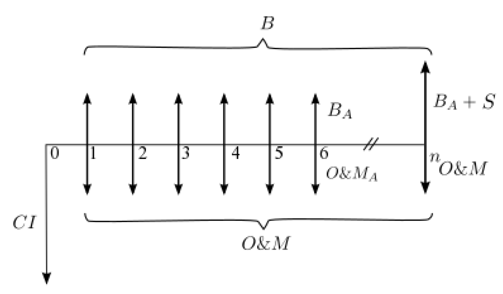
Thus, a project can be analyzed by applying a cash flow model, where the annual incomes and expenses during the project lifetime of
n years are solved to determine the present worth. The simplest model considers the initial cost per kW installed, represented by
; constant annual cash flows related to benefits
; and operation and maintenance costs
. At the end of the project, the salvage value
S is the final income projected. A typical cash flow diagram is presented in
Figure 8.
The net present value (
) of a renewable energy project is a common economic parameter that allows for the development of an economic analysis and determination of its feasibility. Two economic components are identified in the
of a wind energy project: the income, which contains the annual profits due to electricity sales
and a salvage value
at the end of the project; and the expenses, composed of the initial investment
and annual operation and maintenance costs
.
In this analysis, the selected SWTs have different lifetimes, which is a common problem when different technologies are compared. In order to enable comparison, the annual worth is selected as the method of analysis, which converts the typical cash flow described previously into annual equally valued flows (ANPVs). To apply these criteria, the original cash flows are first converted into a single using Equations (9) and (10); then, the are calculated using Equation (11).
After describing the economic model, the next step is to determine each of its defining parameters. Firstly, the initial costs
are described. This parameter takes into account all costs related to installing an SWT, including the electrical infrastructure, conditioning and grid integration, installation, and civil works. The variable is commonly presented as the coefficient of the initial investment cost and the capacity installed [
$/kW]. In
Figure 9, the initial costs of a small wind energy project are presented, with different nominal powers from 2012 to 2015 [
7]. It is observed that the initial costs are reduced when higher nominal power is used. In this context, the installation cost that was used in the economic analysis in this work is
$6040.00 USD/kW.
The annual benefits of the project are considered to be proportional to the AEP and are represented as constant annual cash flows. In Mexico, a domestic user cannot sell energy under the current legal framework. The commercialization scheme is conducted through the exchange of electrons. The domestic renewable energy producer injects its generation into the grid and, when necessary, extracts energy; then, a final balance is calculated at the end of the period. Therefore, the benefits are actually savings that are reflected in electric billing. In order to estimate the savings for a domestic user, it is necessary to know the energy costs, which may not reflect its real generation cost due the subsidy scheme for domestic users in Mexico for certain electricity tariffs.
The cost per kWh is associated with the seasonal and geographic mean temperatures within Mexico, and billing for electric services takes place bimonthly. In the specific case of Mexico City, the cost per kWh for a domestic user ranges from 0.044 to 0.24 USD/kWh for demand of less than 75 kWh to greater than 250 kWh, respectively. These tariffs are known as T1 and Domestic High Consumption (or DAC, per its abbreviation in Spanish), respectively [
60]. T1 and DAC tariffs also represent the higher and lower values of the costs for domestic users. Therefore, these values were selected as the upper and lower limits for the analysis.
It should be noted that the electric domestic tariffs are subsidized in Mexico; however, when electric consumption reaches the DAC level, the tariff subsidy is eliminated, so the real cost of the energy is paid in this scenario. Furthermore, it is important to note that Mexican energy policies do not offer any incentive to include renewable systems for electric generation and/or mitigate CO emissions through electric generation from a renewable energy source for home users.
The Metropolitan Area is formed by Mexico City and certain State of Mexico municipalities and is home to nearly 24 million people, of which almost 6.5 million users represent the domestic feed tariff, representing 5.5 million MWh consumed in 2014 alone [
61,
62]. Therefore, if wind conditions are optimal, there could be a significant number of potential users of
SWT systems. Thus, the present study is relevant for improving the sustainability of the city.
Therefore, the annual benefits
are calculated as presented in Equation (12):
where
is the cost of kWh, and
is the annual energy produced.
The operation and maintenance costs
are considered to be constant cash flows during the project lifetime and, in this work, are calculated as proportional to the initial costs
. We consider this proportionality to be 0.5% [
63]:
The salvage value
S was calculated according to a straight-line depreciation of
[
64]. The annual depreciation
of a wind turbine with initial costs
is expressed by Equation (14):
where
n is the project lifetime. In this analysis,
is considered the salvage value.
5.1.
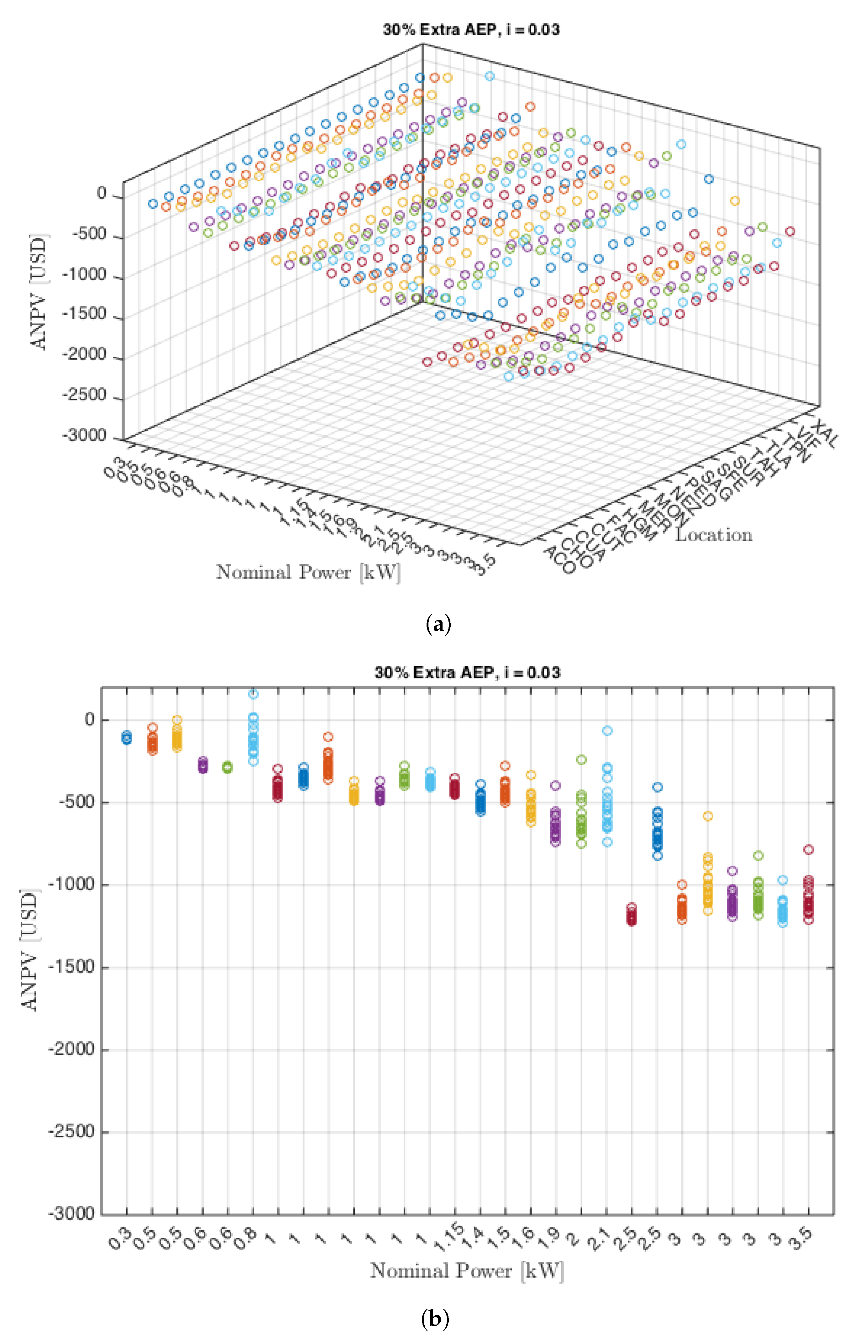
As the first elements of the economic analysis, the were calculated for the 28 SWTs assessed at the 18 sites. The economic conditions selected are the energy costs in a DAC electric tariff. In order to estimate the annual benefits, the is assumed to be constant over the life of the project. The AEP was calculated using the original time series with mean times of 60 min. As the analysis was developed for SWTs in domestic applications, 30% additional energy was applied to the as a first approach to compensating for the underestimation that arises from the sample mean time. Finally, a 3% discount rate was selected.
In
Figure 10a, the calculated
are plotted, represented by ∘, and the colors are associated with a specific
SWT model. The values repeated along the nominal power axis represent different wind turbine models with equal nominal power. This graphical representation was selected to visually compare the economic and technical parameters among
with equal nominal power. The location axis represents the 18 studied sites in alphabetical order. It is observed that
among the locations are similar, which may be explained by the similar wind conditions within the VMMA. In order to observe this behavior, the location axis is eliminated in
Figure 10b.
It is observed that, for most sites, the values calculated are negative. However, there two that exhibit positive , and these are interpreted as annual project incomes. Therefore, although mainly low wind speed conditions exist within the VMMA, an appropriately selected technology and elevated costs per kWh may establish a favorable context in which positive annual incomes are obtained. The nearest zero values—projects assessed with minimal annual losses—are those with having smaller nominal powers.
In order to analyze the general behavior of the calculated
values,
with equal nominal power are grouped and plotted in
Figure 11. It is observed that the two turbines with a nominal power of 0.6 kW exhibit low dispersion within the VMMA, which is a sign of similar economic performance. The two wind turbines with a nominal power of 2.5 kW present a dispersion of 800 [USD], which is the largest for the nominal power sets. Furthermore, for these
, a difference between
is observed, which indicates that, despite the equal nominal power, the annual values differ by nearly 400 USD.
In order to observe
dispersion for a specific nominal power,
Figure 12 presents the probability plots of the seven turbine models with a nominal power of 1 kW. The wind turbines with the highest and lowest
within the VMMA are the third and fifth, respectively (From left to right). The seventh
exhibits minimum dispersion, which may be interpreted as persistent power production at all locations.
Thus, although nominal power provides a technical characteristic for classifying wind turbines, it is observed that wind turbines with equal nominal power exhibit different economic performances. Therefore, in order to develop reliable techno-economic studies, the methodology should include a comparison of technologies with equal or similar nominal power values in order to carry out an appropriate technology selection.
5.2. Capacity Factor
The capacity factor is a common parameter used to report SWT power generation performance. It is calculated with the ratio of the real wind turbine production and the production assuming nominal generation for a period of 1 year.
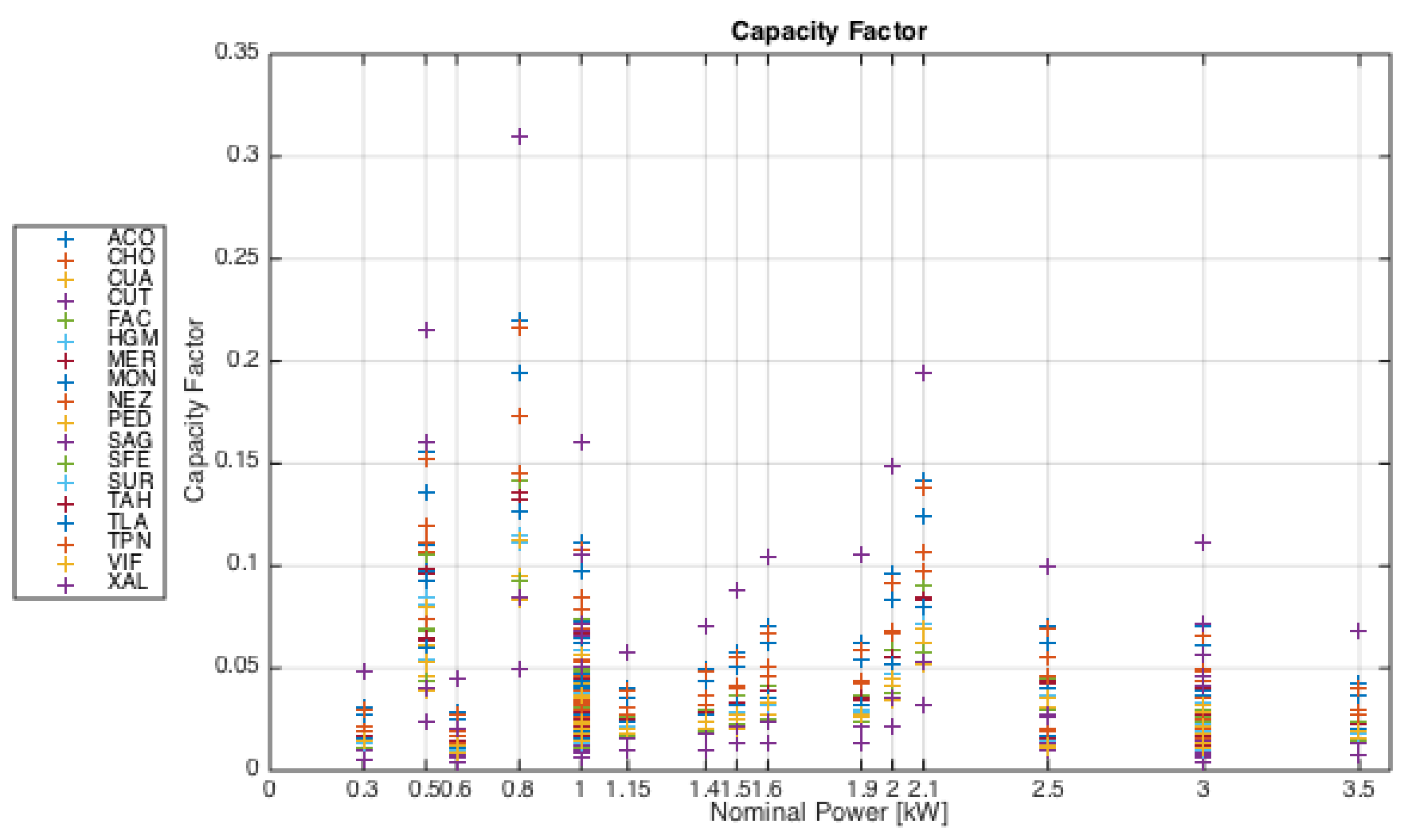
Preserving the order of nominal power and sites from
Figure 10,
Figure 13 presents the
values for the 28 sites and 18
SWTs. It is observed that, although wind conditions are similar within the VMMA, power performance results from a relationship between the wind conditions and characteristics of the technology represented by the power curve. For example, the
with a nominal power of 0.8 kW exhibits a
between 5 and 31%. This is one of the
previously calculated with positive values. Therefore, the appropriate selection of an
is a determining factor for defining project feasibility. This variability in
values by location and wind turbine was also observed in the Greater London area [
11].
After observing the individual
power performances, wind turbines with equal nominal power values were grouped and plotted. In
Figure 14, it is observed that a
higher than 20% corresponds to wind turbines with nominal powers of 0.5, 0.8, and 2.1 kW. The first two correspond to technologies with a positive
, while the latter corresponds to the negative
that is nearest to zero among the turbines evaluated. The manner in which power performance changes with wind conditions is also observed.
From
Table 2, it follows that similar wind conditions are present in the VMMA; however, the capacity factor and
change according to the wind parameters and the power curve. In order to establish a relation between
and
, the axis corresponding to the sites is removed. The resulting graph is presented in
Figure 15. It preserves the order of nominal power of
Figure 11 and
Figure 14, and
and
are plotted and represented by the symbols ∘ and +, respectively. The colors are preserved in order to identify locations. It is observed that, in general,
does not change among locations; however, there are certain locations, namely
and
, that exhibit the highest values.
The values calculated exhibit similar behavior among sites, while most of the assessed technologies exhibit negative values. However, the SWT with a nominal power of 0.8 kW has positive values, and for these scenarios, the calculated are above 20%—a value that defines the threshold for obtaining a positive . Furthermore, the wind turbine with a nominal power of 2.1 kW exhibits an that is equal to zero for one location. Therefore, although wind conditions are similar within the VMMA, SWT performance is a key factor in power production; therefore, reliable methodologies are required for the correct characterization of wind turbine power production.
In order to understand the differences in
and
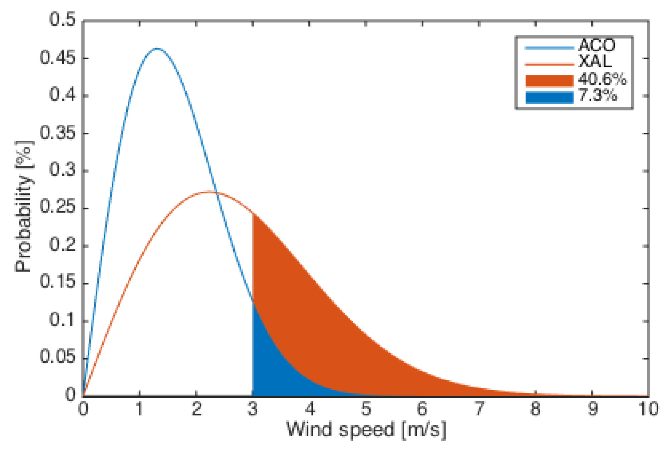
among the assessed sites, the two locations with the maximum and minimum values of expected wind speeds were selected:
and
. A common technical characteristic of the selected
is the drop in wind speed at 3 m/s.
Figure 16 presents the two Rayleigh distributions of these locations and the probabilities of having wind speeds higher than the cut in wind speed.
As observed in
Figure 16 for the
and
locations, these probabilities are 7.3% and 40.6%, respectively. Therefore, although the expected wind speeds are very similar, as can be observed in
Table 2, the model shape and compatibility with the power curve are factors that determine the
and, consequently, project reliability.
5.3. CO2 Mitigation
An important aspect of power generation through a renewable energy source, such as wind power, is the mitigation of greenhouse gas emissions. These environmental effects are quantifiable and provide additional information regarding project benefits. This information is commonly used by governments to implement economic strategies to promote renewable energy generation.
A common strategy for promoting renewable energy is to associate a substitute price with preventing CO
2 emissions [
65]. This cost is used as an incentive because it associates economic benefits with each kWh generated by a renewable energy source.
According to the Secretariat of Environment and Natural Resources (SEMARNAT), the emission factor for electric generation in 2015 was evaluated to be 0.458 ; therefore, it is possible to estimate mitigation from the for each .
It is important to mention that, although the methodology presented was developed in an economic context, another method by which to include positive environmental effects is to associate an additional benefit gained from generating electricity through wind turbines: mitigating greenhouse emissions. In order to do so, the annual income per ton of CO
2 mitigated is considered. Recent studies have projected that the cost per ton of CO
2 in 2020 will be
$43.00 USD [
65]. Thus,
Figure 17 presents the result of considering this additional income for a group of wind turbines using the closest values to zero. An alternative strategy to improve project feasibility was used in Italy. Regulations allow for subsidizing measures that provide extra benefits in the form of income per kWh generated [
13].
In
Figure 17, it is observed that the general tendency is for the
to increase; however, the number of projects evaluated with positive
remains: only the two wind turbines (with nominal powers of 0.5 and 0.8 kW) exhibit positive values. The wind turbine with a nominal power of 2.1 kW at the
location reduces the total annual loss, but the value remains negative.
6. Conclusions
In this work, we calculated the annual energy produced (AEP) for a set of 28 small wind turbines (SWTs) with nominal powers between 0.3 and 3.5 kW at 18 locations within the Valley of Mexico Metropolitan Area (VMMA). An adjustment to the power production was implemented due to the mean time of the time series used in the resource assessment. Furthermore, a techno-economic analysis was developed using the annual net present value (ANPV) technique in order to evaluate project feasibility. To apply this methodology, a scenario with the given the electrical context for a domestic consumer in the VMMA was explored. To show the economic effects while considering annual benefits by means of greenhouse gas mitigation, extra income added to the ANPV is proposed.
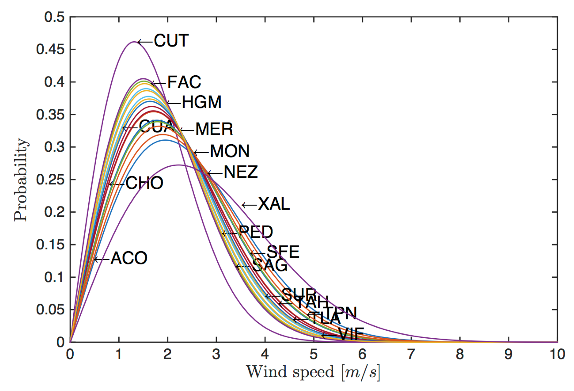
The Rayleigh probability density function (PDF) was selected to model all wind speed data sets, and it was observed that expected wind speeds range between 1.65 and 2.79 m/s, corresponding to the Acolman (ACO) and Xalostoc (XAL) locations, respectively. However, if an SWT’s wind speed drops below 3 m/s, the difference between power production probabilities for both sites is 33.3%.
In the catalog of wind turbines used, certain devices exhibit equal nominal power. After developing the ANPV and capacity factor (CF) studies, results are found to differ among turbines with equal nominal power and similar wind conditions. Therefore, for the SWTs studied, nominal power may not be a standard technical parameter for describing SWT power production.
In order to conduct reliable techno-economic studies, the methodology should include a comparison of technologies with equal or similar nominal powers to make an appropriate technology selection.
Although wind conditions are similar within the VMMA, two technologies exhibit annual incomes. The power performance of an SWT is only represented by its power curve; therefore, it is necessary to develop reliable methodologies to correctly characterize wind turbine power production.
ANPV as the economic methodological basis of assessing reliability allows for the comparison of technologies with different lifetimes. Furthermore, to complement the ANPV results, a CO2 mitigation analysis is presented, thus establishing relationships between kWh generated by the SWT, tons of CO2 mitigated, and cost per ton of CO2. This methodology allows for the inclusion of an environmental mechanism to promote the penetration of these technologies, and the way in which these benefits may be included in the final results is demonstrated.

 ,
, 


