Experimental Identification of the Optimal Current Vectors for a Permanent-Magnet Synchronous Machine in Wave Energy Converters


Abstract
1. Introduction
1.1. Motivation
1.2. Contribution of the Paper
1.3. Outline of the Paper
2. Theory
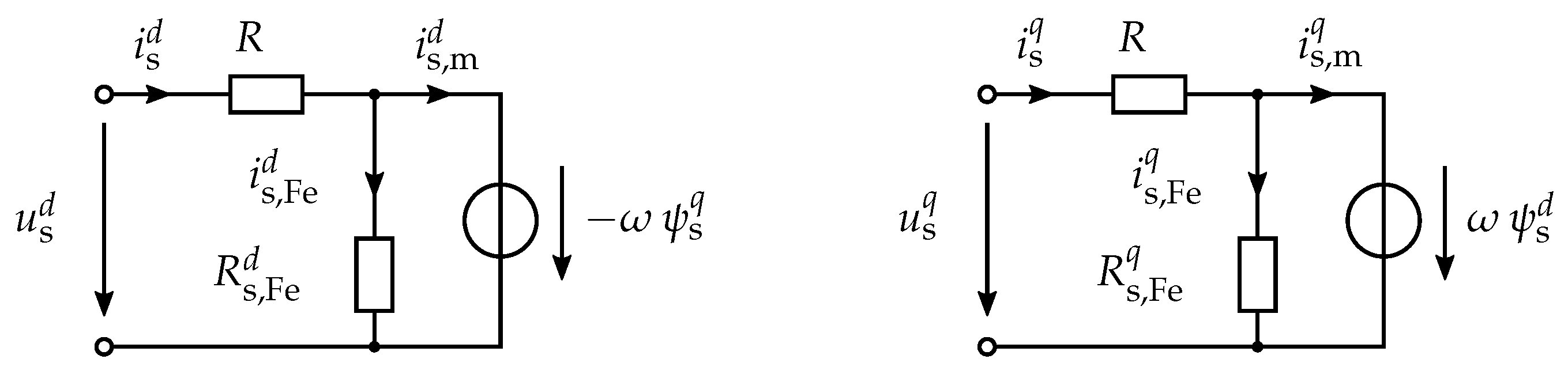
2.1. Model of a Synchronous Machine without Iron Losses
- The three phases of the electrical machine are star-connected (i.e., ).
- The machine is symmetrical.
- Only the fundamentals are considered and spatial harmonics are neglected.
- Iron losses are neglected.
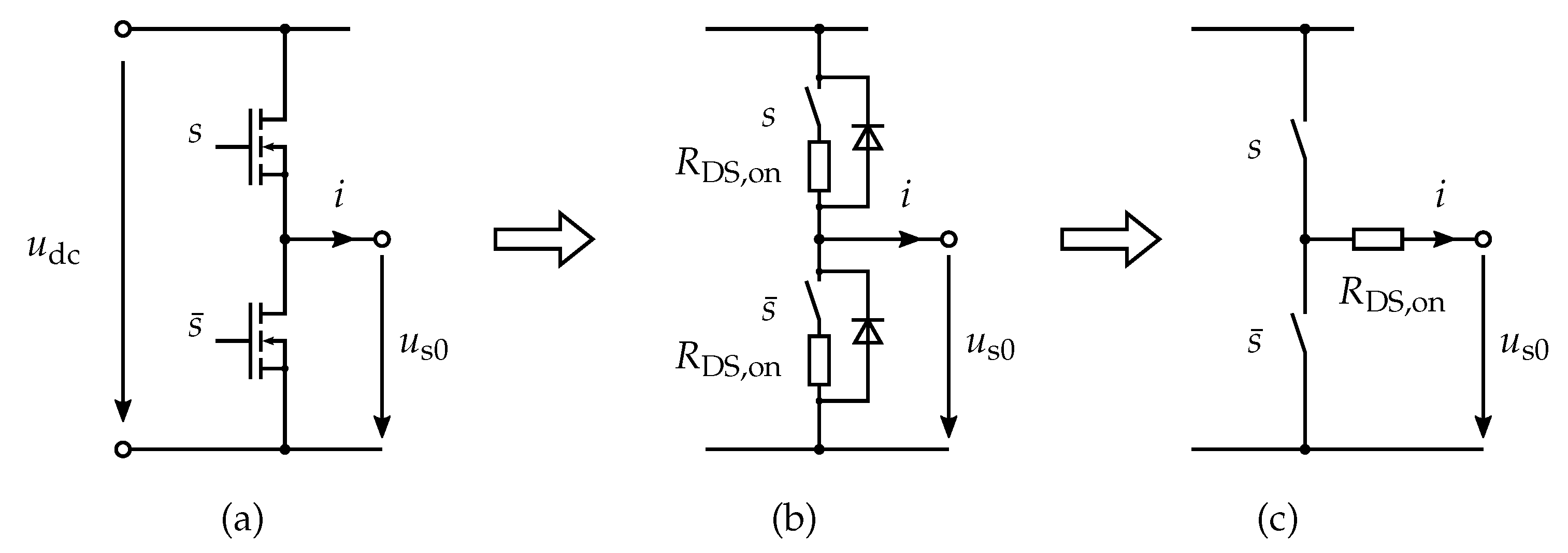
2.2. Simplified Modelling of the Voltage Source Inverter
2.3. Power Analysis
3. Methods for Efficiency Enhancement
3.1. Maximum Torque Per Current for Linear Flux Linkages
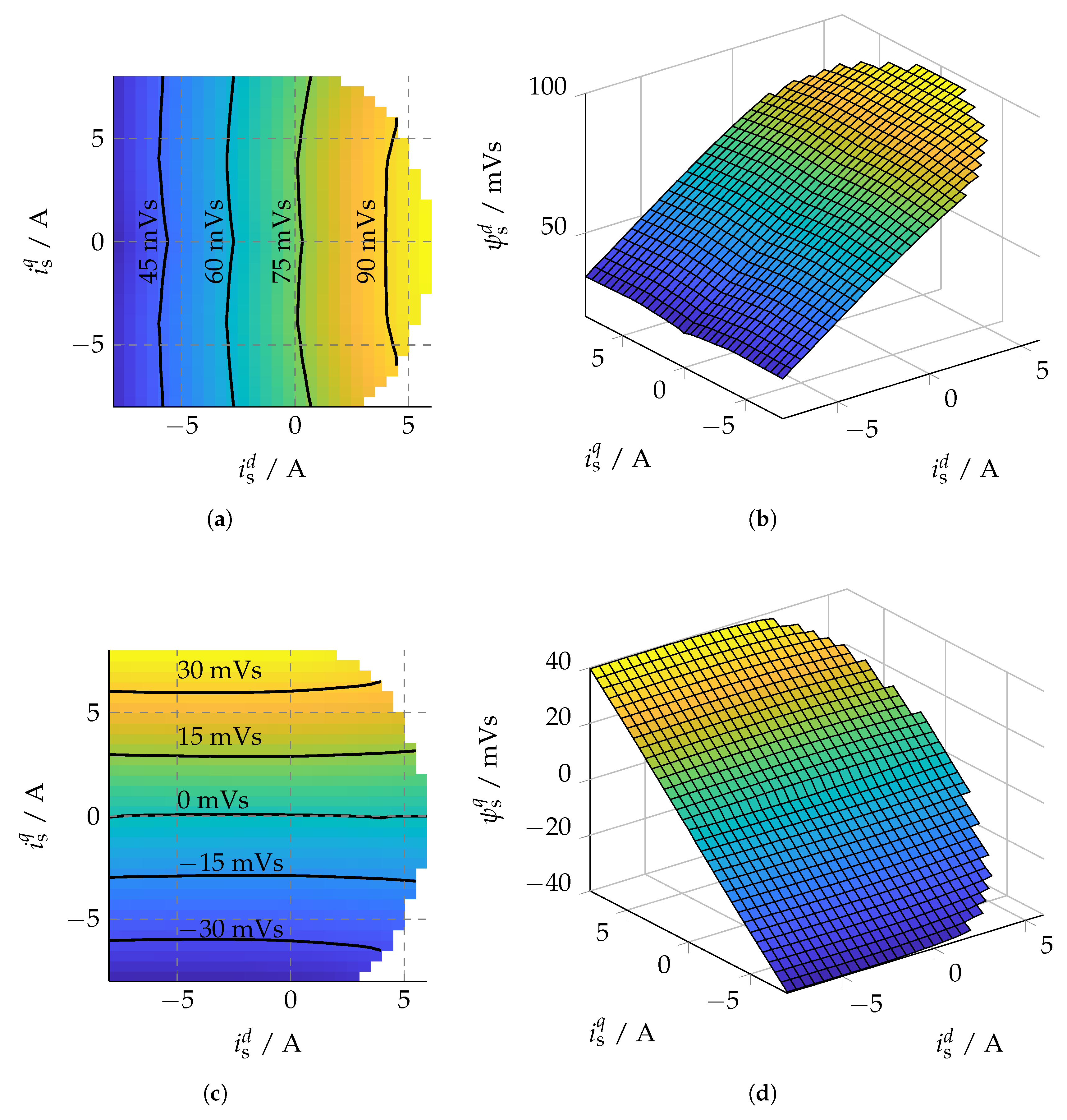
3.2. Maximum Torque Per Current for Nonlinear Flux Linkages
3.3. Direct Measurement of the Current Vector with the Maximum Efficiency
4. Implementation and Measurements
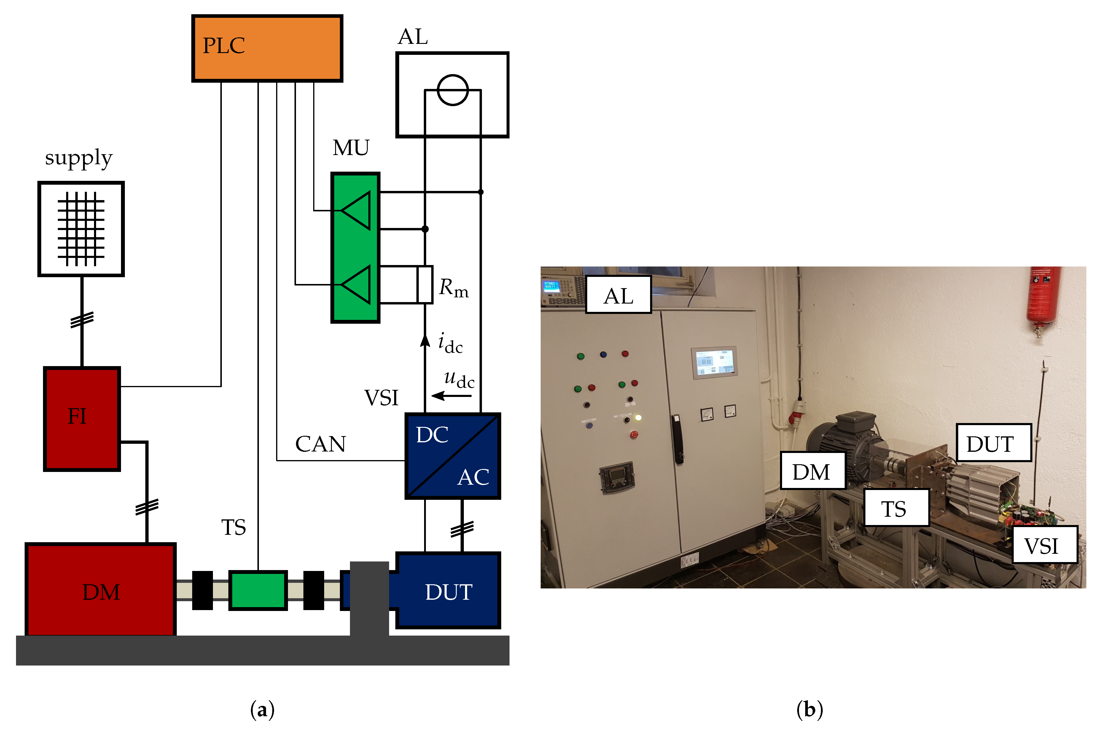
4.1. Setup of the Test Bench
4.2. Measurement Results
5. Conclusions
Author Contributions
Funding
Conflicts of Interest
References
- Eldeeb, H.; Hackl, C.M.; Horlbeck, L.; Kullick, J. A unified theory for optimal feedforward torque control of anisotropic synchronous machines. Int. J. Control 2017, 1–30. [Google Scholar] [CrossRef]
- Schröder, D. Elektrische Antriebe—Regelung von Antriebssystemen, 4th ed.; Springer: Berlin/Heidelberg, Germany, 2015. [Google Scholar]
- Rang, G.; Lim, J.; Nam, K.; Ihm, H.B.; Kim, H.G. A MTPA Control Scheme for an IPM Synchronous Motor Considering Magnet Flux Variation Caused by Temperature. In Proceedings of the Nineteenth Annual IEEE Applied Power Electronics Conference and Exposition, 2004 (APEC ’04), Anaheim, CA, USA, 22–26 February 2004; Volume 3, pp. 1617–1621. [Google Scholar] [CrossRef]
- Jung, S.; Hong, J.; Nam, K. Current Minimizing Torque Control of the IPMSM Using Ferrari’s Method. IEEE Trans. Power Electron. 2013, 28, 5603–5617. [Google Scholar] [CrossRef]
- Hoang, K.D.; Wang, J.; Cyriacks, M.; Melkonyan, A.; Kriegel, K. Feed-forward Torque Control of Interior Permanent Magnet Brushless AC Drive for Traction Applications. In Proceedings of the 2013 International Electric Machines Drives Conference, Chicago, IL, USA, 12–15 May 2013; pp. 152–159. [Google Scholar] [CrossRef]
- Mekri, F.; Elghali, S.B.; Benbouzid, M.E.H. Fault-Tolerant Control Performance Comparison of Three- and Five-Phase PMSG for Marine Current Turbine Applications. IEEE Trans. Sustain. Energy 2013, 4, 425–433. [Google Scholar] [CrossRef]
- Mekri, F.; Charpentier, J.; Benelghali, S.; Kestelyn, X. High Order Sliding mode optimal current control of five phase permanent magnet motor under open circuited phase fault conditions. In Proceedings of the 2010 IEEE Vehicle Power and Propulsion Conference, Lille, France, 1–3 September 2010; pp. 1–6. [Google Scholar] [CrossRef]
- Kestelyn, X.; Semail, E. A Vectorial Approach for Generation of Optimal Current References for Multiphase Permanent-Magnet Synchronous Machines in Real Time. IEEE Trans. Ind. Electron. 2011, 58, 5057–5065. [Google Scholar] [CrossRef]
- Bolognani, S.; Petrella, R.; Prearo, A.; Sgarbossa, L. Automatic Tracking of MTPA Trajectory in IPM Motor Drives Based on AC Current Injection. IEEE Trans. Ind. Appl. 2011, 47, 105–114. [Google Scholar] [CrossRef]
- Kim, S.; Yoon, Y.; Sul, S.; Ide, K. Maximum Torque per Ampere (MTPA) Control of an IPM Machine Based on Signal Injection Considering Inductance Saturation. IEEE Trans. Power Electron. 2013, 28, 488–497. [Google Scholar] [CrossRef]
- Sun, T.; Wang, J.; Chen, X. Maximum Torque Per Ampere (MTPA) Control for Interior Permanent Magnet Synchronous Machine Drives Based on Virtual Signal Injection. IEEE Trans. Power Electron. 2015, 30, 5036–5045. [Google Scholar] [CrossRef]
- Ahmed, A.; Sozer, Y.; Hamdan, M. Maximum Torque per Ampere Control for Interior Permanent Magnet Motors using DC Link Power Measurement. In Proceedings of the 2014 IEEE Applied Power Electronics Conference and Exposition—APEC 2014, Fort Worth, TX, USA, 6–20 March 2014; pp. 826–832. [Google Scholar] [CrossRef]
- Armando, E.; Bojoi, R.I.; Guglielmi, P.; Pellegrino, G.; Pastorelli, M. Experimental Identification of the Magnetic Model of Synchronous Machines. IEEE Trans. Ind. Appl. 2013, 49, 2116–2125. [Google Scholar] [CrossRef]
- Mink, F.; Kubasiak, N.; Ritter, B.; Binder, A. Parametric Model and Identification of PMSM Considering the Influence of Magnetic Saturation. In Proceedings of the 2012 13th International Conference on Optimization of Electrical and Electronic Equipment (OPTIM), Brasov, Romania, 24–26 May 2012; pp. 444–452. [Google Scholar] [CrossRef]
- Kellner, S.L.; Seilmeier, M.; Piepenbreier, B. Impact of Iron Losses on Parameter Identification of Permanent Magnet Synchronous Machines. In Proceedings of the 2011 1st International Electric Drives Production Conference, Nuremberg, Germany, 28–29 September 2011; pp. 11–16. [Google Scholar] [CrossRef]
- Richter, J.; Dollinger, A.; Doppelbauer, M. Iron Loss and Parameter Measurement of Permanent Magnet Synchronous Machine. In Proceedings of the 2014 International Conference on Electrical Machines (ICEM), Berlin, Germany, 2–5 September 2014; pp. 1635–1641. [Google Scholar] [CrossRef]
- Morimoto, S.; Tong, Y.; Takeda, Y.; Hirasa, T. Loss Minimization Control of Permanent Magnet Synchronous Motor Drives. IEEE Trans. Ind. Electron. 1994, 41, 511–517. [Google Scholar] [CrossRef]
- Uddin, M.N.; Zou, H.; Azevedo, F. Online Loss Minimization Based Adaptive Flux Observer for Direct Torque and Flux Control of PMSM Drive. In Proceedings of the 2014 IEEE Industry Application Society Annual Meeting, Vancouver, BC, Canada, 5–9 October 2014; pp. 1–7. [Google Scholar] [CrossRef]
- Barisa, T.; Sumina, D.; Kutija, M. Comparison of Maximum Torque per Ampere and Loss Minimization Control for the Interior Permanent Magnet Synchronous Generator. In Proceedings of the 2015 International Conference on Electrical Drives and Power Electronics (EDPE), Tatranska Lomnica, Slovakia, 21–23 September 2015; pp. 497–502. [Google Scholar]
- Pairo, H.; Shoulaie, A. Effective and simplified method in maximum efficiency control of interior permanent magnet synchronous motors. IET Electr. Power Appl. 2017, 11, 447–459. [Google Scholar] [CrossRef]
- Dirscherl, C.; Hackl, C.; Schechner, K. Modellierung und Regelung von modernen Windkraftanlagen: Eine Einführung. In Elektrische Antriebe—Regelung von Antriebssystemen; Schröder, D., Ed.; Springer: Berlin/Heidelberg, Germany, 2015; Chapter 24; pp. 1540–1614. [Google Scholar]
- Richter, J.; Gemaßmer, T.; Doppelbauer, M. Predictive Current Control of Saturated Cross-Coupled Permanent Magnet Synchronous Machines. In Proceedings of the 2014 International Symposium on Power Electronics, Electrical Drives, Automation and Motion, Ischia, Italy, 18–20 June 2014; pp. 830–835. [Google Scholar] [CrossRef]
- Wittig, B. Verbesserung des Schalt- und Betriebsverhaltens von Leistungs-MOSFETs mit niedriger Spannungsfestigkeit und hoher Stromtragfähigkeit durch Optimierung der Treiberschaltung. Ph.D. Thesis, Christian-Albrechts-Universität zu Kiel, Kiel, Germany, 2012. [Google Scholar]
- Wintrich, A.; Nicolai, U.; Tursky, W.; Reimann, T. Applikationshandbuch Leistungshalbleiter, 2nd ed.; ISLE Verlag: Ilmenau, Germany, 2015. [Google Scholar]
- Hackl, C.M.; Kamper, M.J.; Kullick, J.; Mitchell, J. Current control of reluctance synchronous machines with online adjustment of the controller parameters. In Proceedings of the 2016 IEEE 25th International Symposium on Industrial Electronics (ISIE), Santa Clara, CA, USA, 8–10 June 2016; pp. 153–160. [Google Scholar] [CrossRef]
- Hackl, C.M. Non-Identifier Based Adaptive Control in Mechatronics; Springer International Publishing: Basel, Switzerland, 2017. [Google Scholar]
- Xu, L.; Yao, J. A Compensated Vector Control Scheme of a Synchronous Reluctance Motor Including Saturation and Iron Losses. IEEE Trans. Ind. Appl. 1992, 28, 1330–1338. [Google Scholar] [CrossRef]


 ), the current limit (
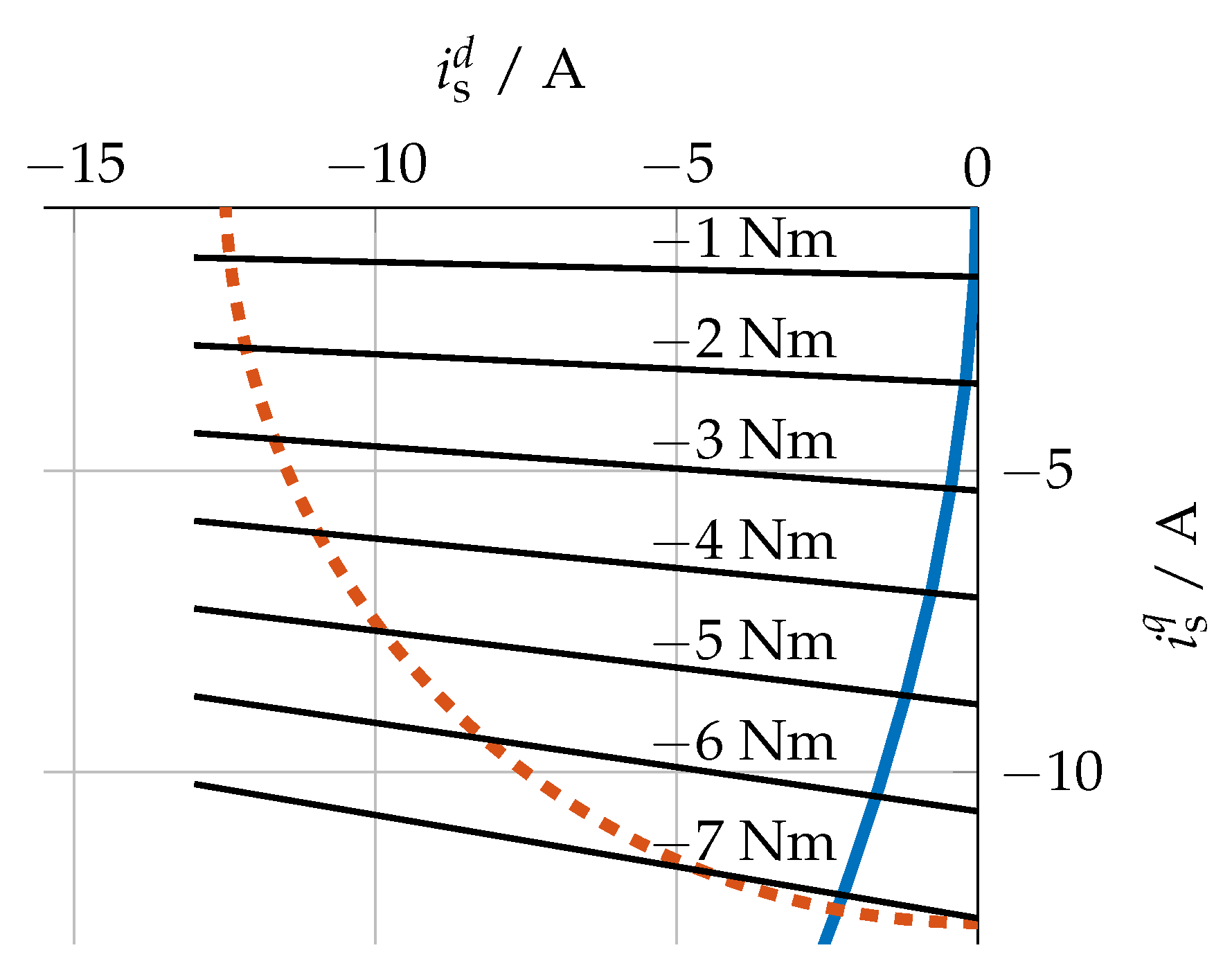
 ), and the numerically calculated Maximum Torque per Current (MTPC) hyperbola with linearised flux linkages (
 ).
), the current limit (), and the numerically calculated Maximum Torque per Current (MTPC) hyperbola with linearised flux linkages ().
).
), the current limit (), and the numerically calculated Maximum Torque per Current (MTPC) hyperbola with linearised flux linkages ().
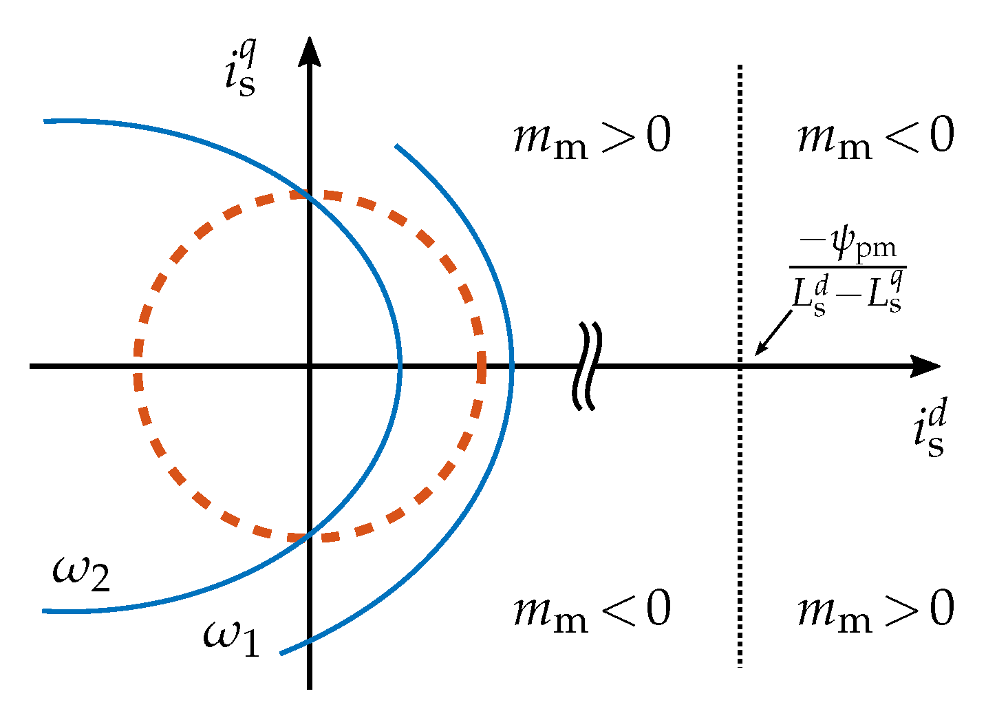
 ), the current limit (), and the voltage limit () for two different speeds .
), the current limit (), and the voltage limit () for two different speeds .
), the current limit (), and the voltage limit () for two different speeds .

 ) and fitted polynomial of second order () over the direct current for a constant torque of .
) and fitted polynomial of second order () over the direct current for a constant torque of .
) and fitted polynomial of second order () over the direct current for a constant torque of .
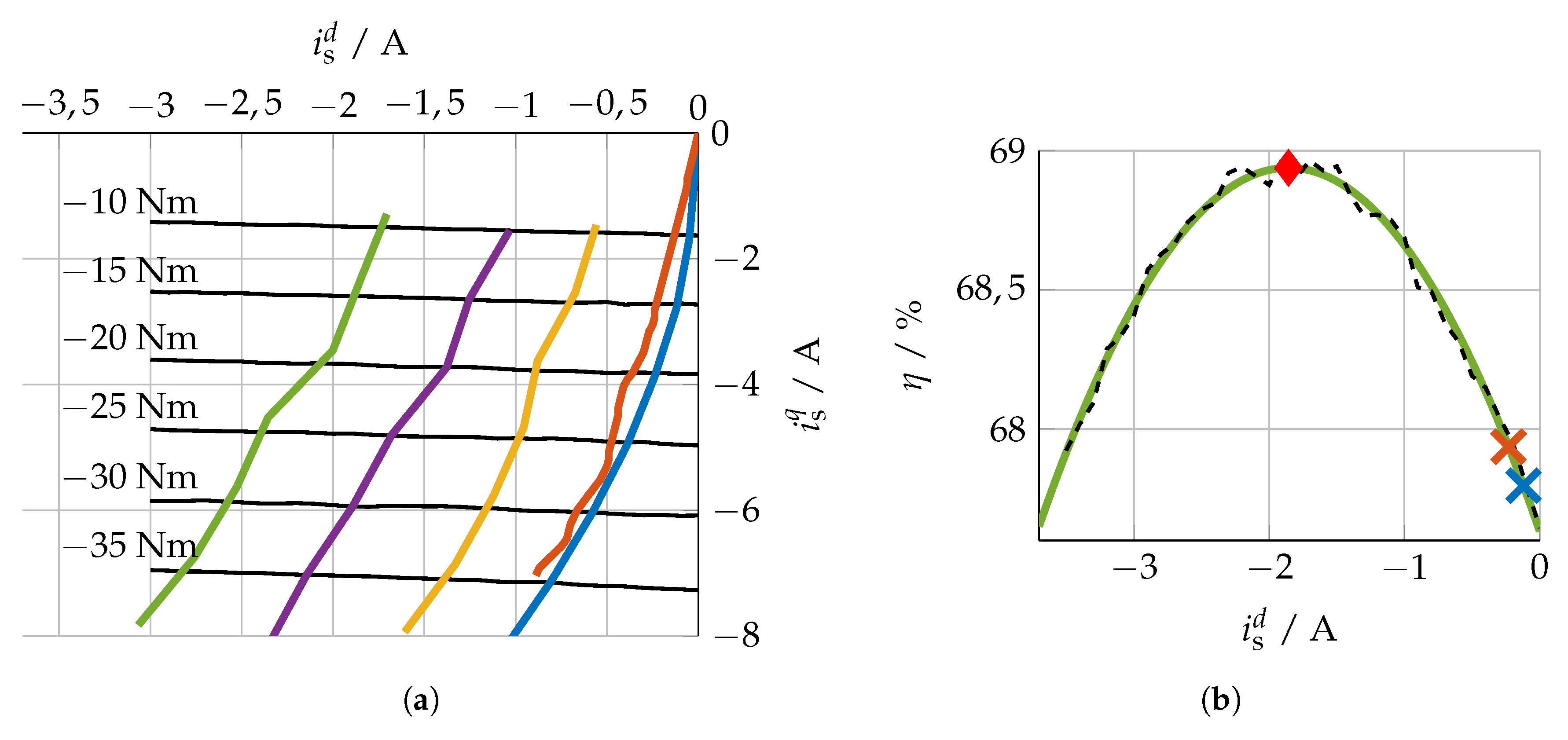
 ) and resulting trajectories for the two MTPC methods with linear approximated () and nonlinear (
 ) flux linkages and the measured trajectories with the maximum efficiency for different shaft speeds of (
 ), (
), ( ), and (
 ) in the ()-plane. (b) Efficiency () for a shaft speed of and a constant torque of and the two points of MTPC for linear approximated (
 ) and nonlinear (
 ) flux linkages and the point of maximum efficiency (
 ).
) and resulting trajectories for the two MTPC methods with linear approximated () and nonlinear () flux linkages and the measured trajectories with the maximum efficiency for different shaft speeds of (), (), and () in the ()-plane. (b) Efficiency () for a shaft speed of and a constant torque of and the two points of MTPC for linear approximated () and nonlinear () flux linkages and the point of maximum efficiency ().
).
) and resulting trajectories for the two MTPC methods with linear approximated () and nonlinear () flux linkages and the measured trajectories with the maximum efficiency for different shaft speeds of (), (), and () in the ()-plane. (b) Efficiency () for a shaft speed of and a constant torque of and the two points of MTPC for linear approximated () and nonlinear () flux linkages and the point of maximum efficiency ().


| Name | Parameter | Value |
|---|---|---|
| Number of pole pairs | 5 | |
| Gear ratio | 8 | |
| Stator resistance at | ||
| Stator resistance at | ||
| Drain-source on resistance | ||
| Resistance of the cable | ||
| Permanent-magnet flux linkage | ||
| d-Inductance | ||
| q-Inductance |
© 2019 by the authors. Licensee MDPI, Basel, Switzerland. This article is an open access article distributed under the terms and conditions of the Creative Commons Attribution (CC BY) license (http://creativecommons.org/licenses/by/4.0/).
Share and Cite
Krüner, S.; Hackl, C.M. Experimental Identification of the Optimal Current Vectors for a Permanent-Magnet Synchronous Machine in Wave Energy Converters. Energies 2019, 12, 862. https://doi.org/10.3390/en12050862
Krüner S, Hackl CM. Experimental Identification of the Optimal Current Vectors for a Permanent-Magnet Synchronous Machine in Wave Energy Converters. Energies. 2019; 12(5):862. https://doi.org/10.3390/en12050862
Chicago/Turabian StyleKrüner, Simon, and Christoph M. Hackl. 2019. "Experimental Identification of the Optimal Current Vectors for a Permanent-Magnet Synchronous Machine in Wave Energy Converters" Energies 12, no. 5: 862. https://doi.org/10.3390/en12050862
APA StyleKrüner, S., & Hackl, C. M. (2019). Experimental Identification of the Optimal Current Vectors for a Permanent-Magnet Synchronous Machine in Wave Energy Converters. Energies, 12(5), 862. https://doi.org/10.3390/en12050862