Agent-Based Modeling of a Thermal Energy Transition in the Built Environment


Abstract
1. Introduction
2. Definition of the Conceptual Framework
2.1. Sociotechnical Systems (STS)
2.2. Complex Adaptive Systems (CAS)
2.3. Basic Notions of Agent-Based Modeling
3. Materials and Methods
3.1. Model Development
3.2. Computational Simulations
3.3. Analysis of Results
4. Illustrative Example: from Natural Gas-Based to Natural Gas-Free Heating in Residential Neighborhoods
4.1. The Thermal Energy Transition through the Lenses of STS and CAS
4.2. Model Overview
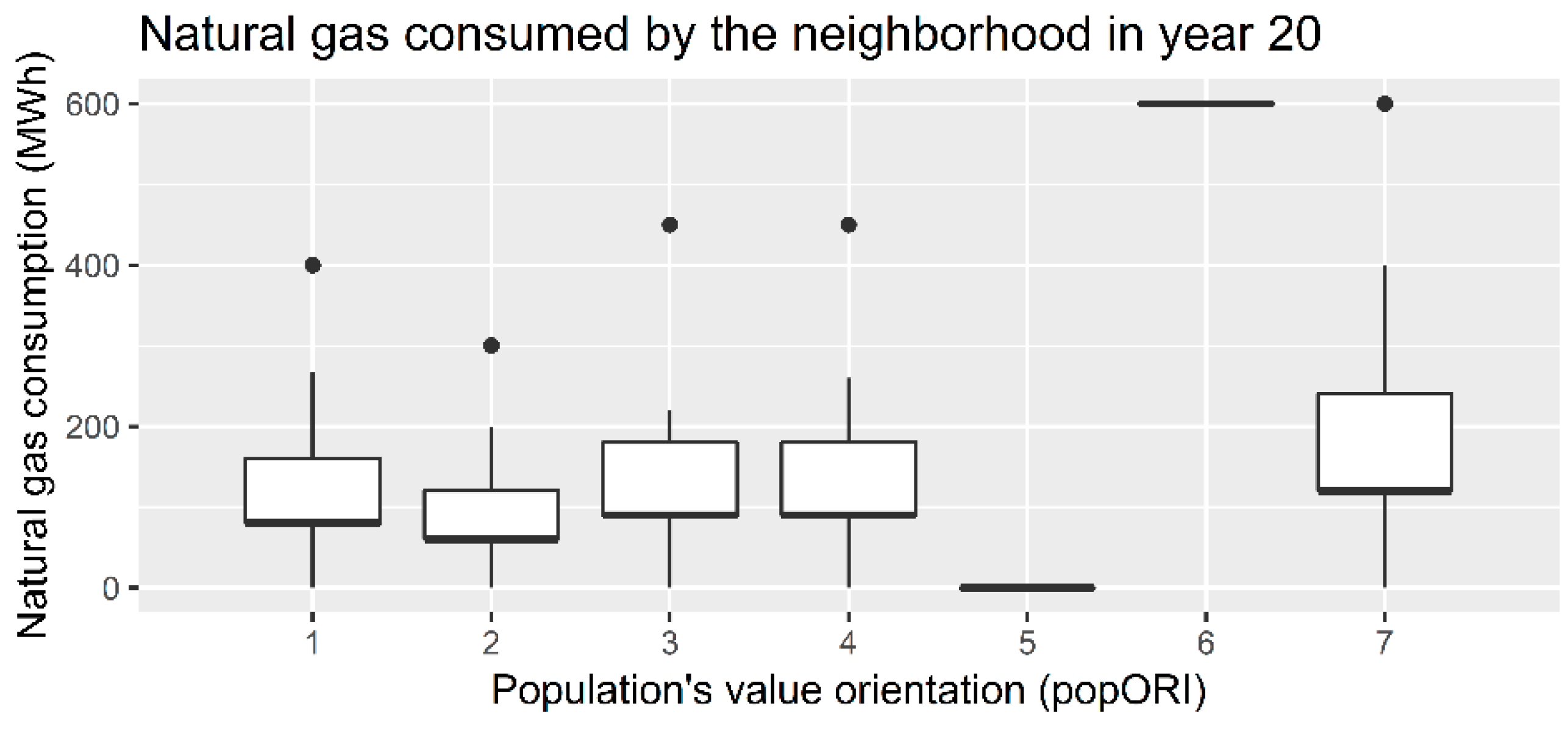
- Under which socioeconomic conditions did the neighborhood transition fully to natural gas-free heating?
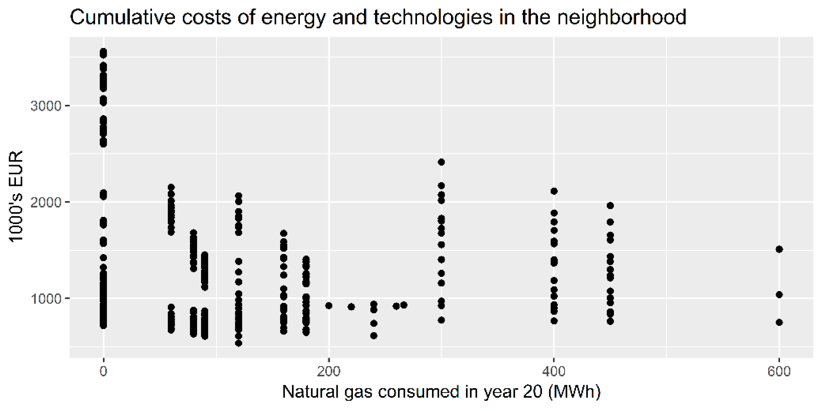
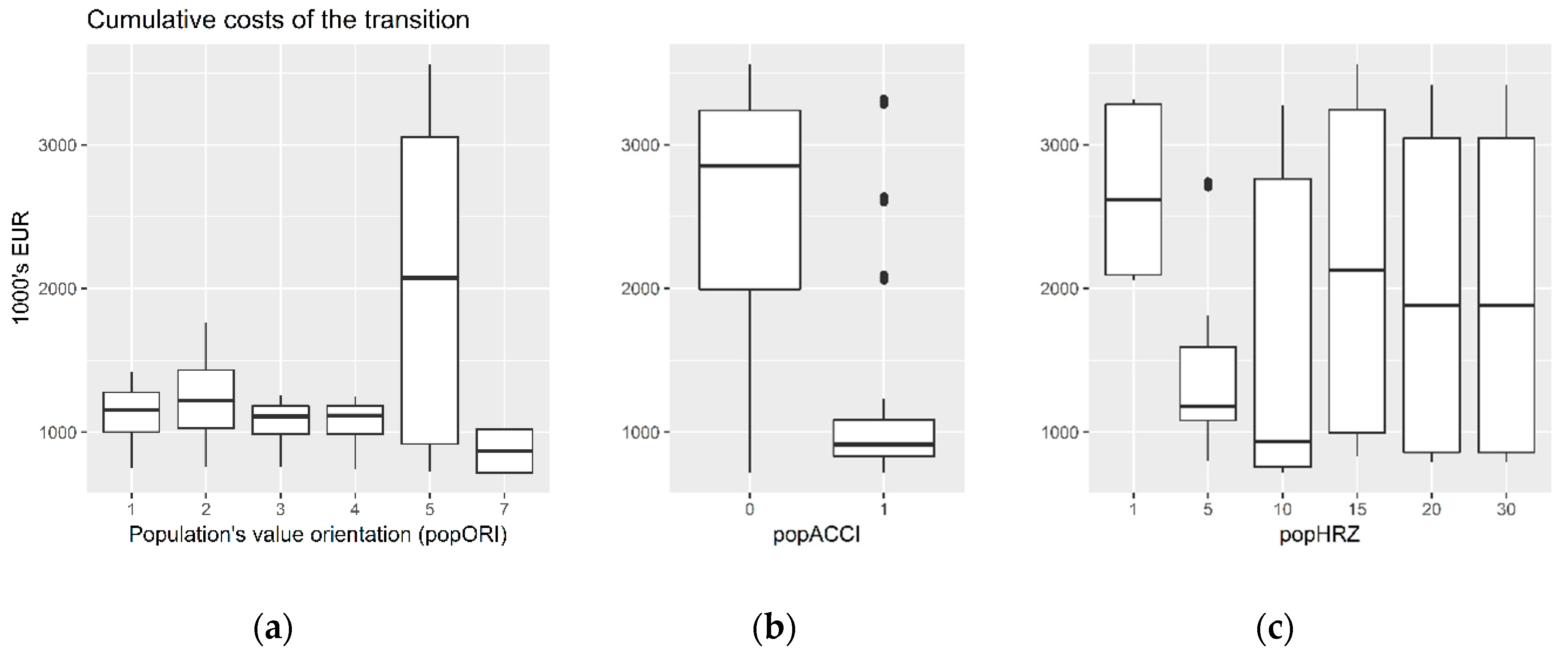
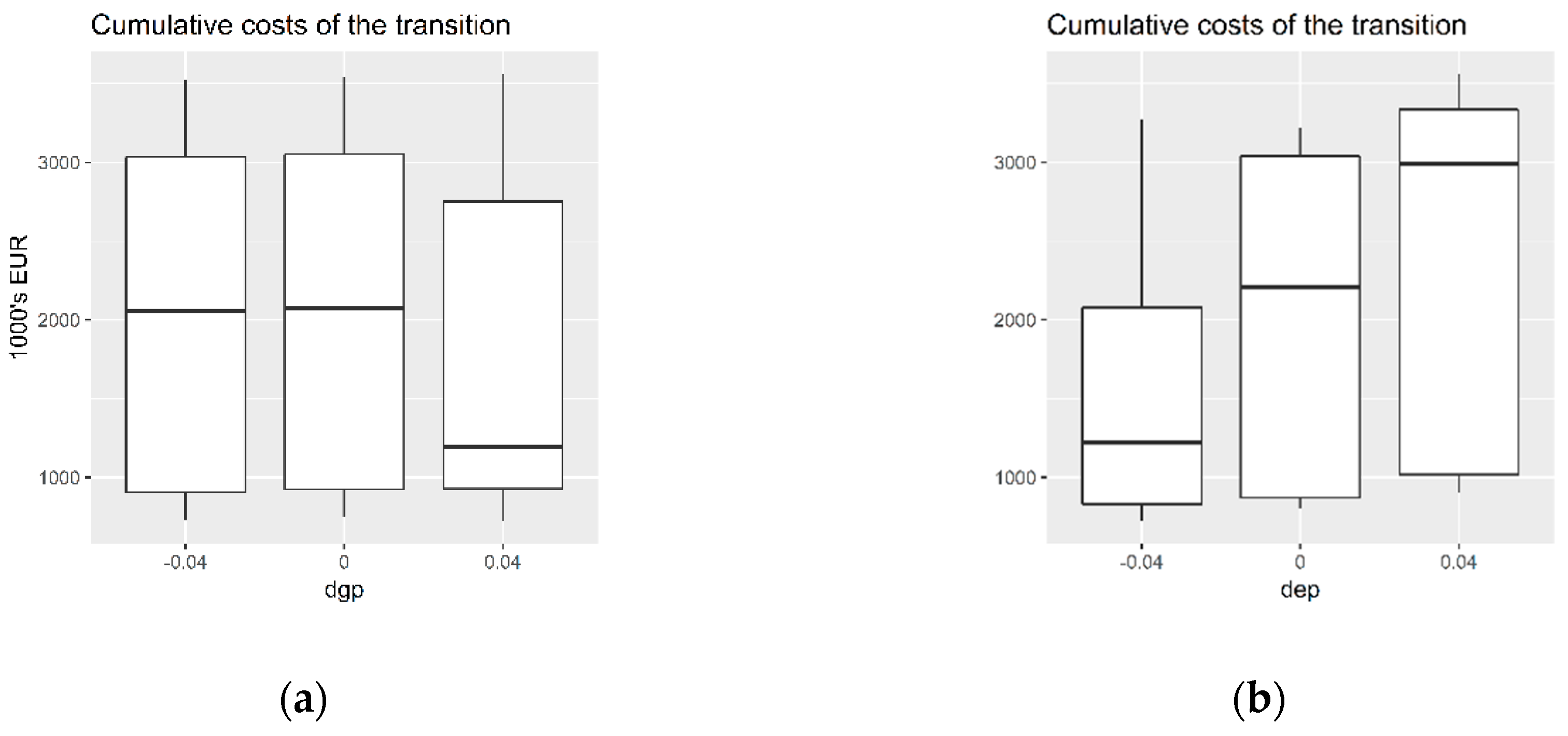
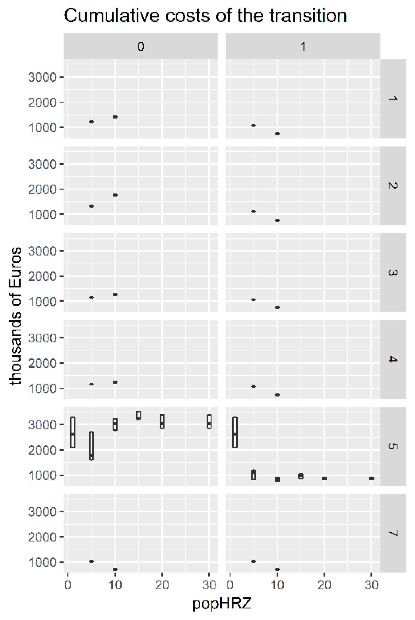
- What were the costs of the transition?
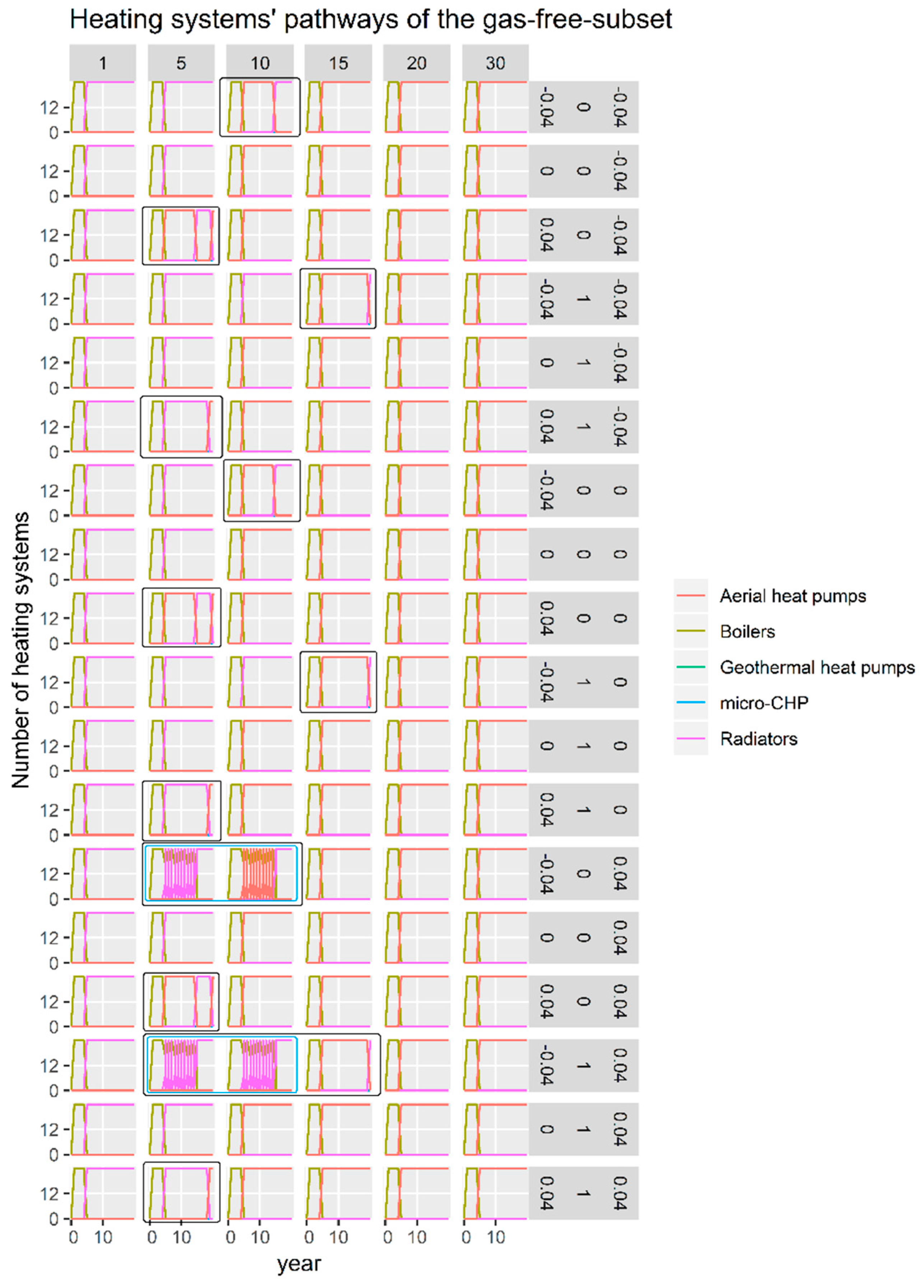
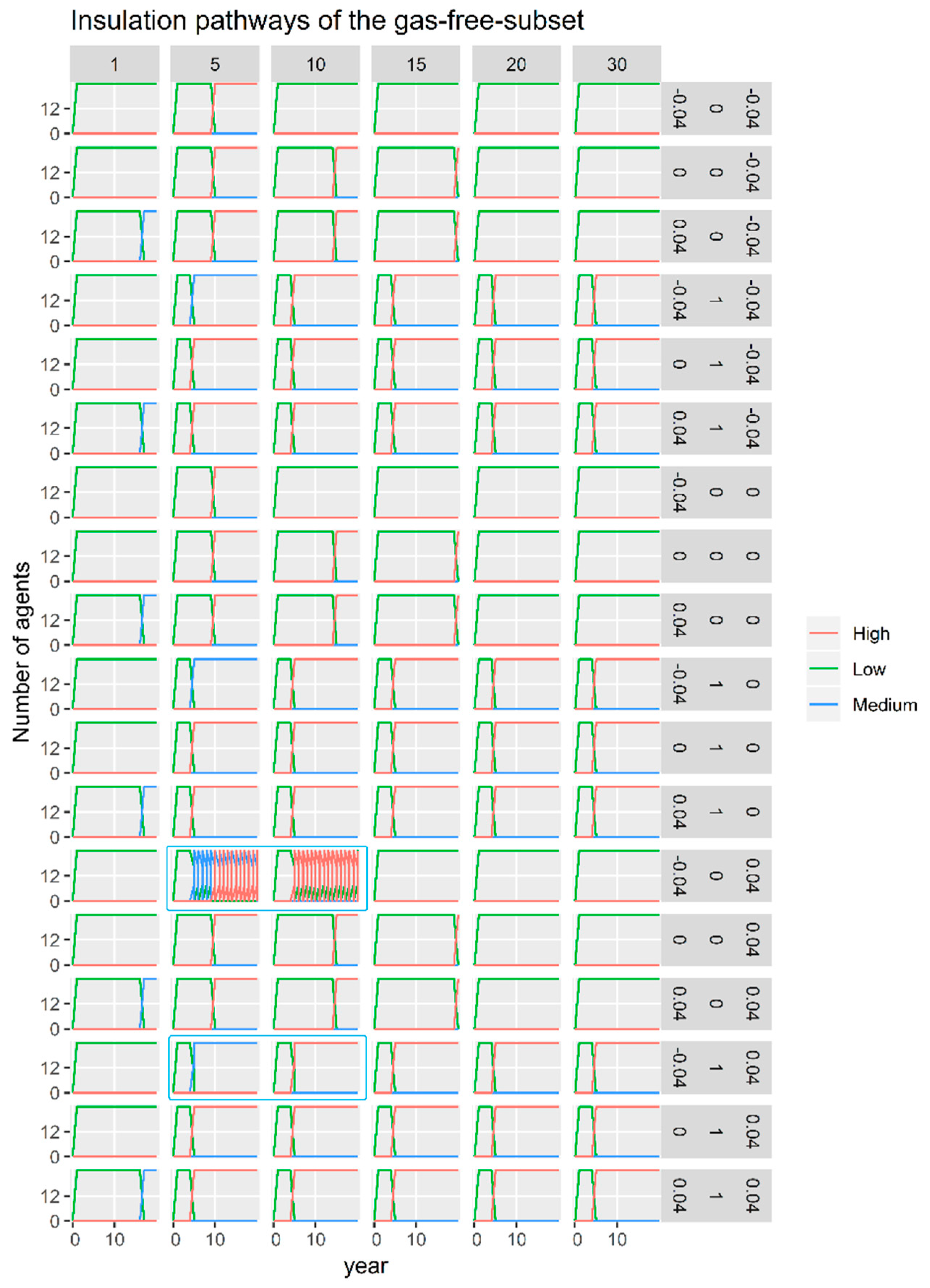
- Which changes in household insulation and heating systems took place during these transitions?
4.2.1. Model Entities, State Variables, and Scale
- Equation (1) applies to technologies that consume natural gas and not electricity.
- In Equation (2), information regarding maintenance costs and investment costs is part of the environment and is available to agents.
- In Equation (3), annual demand is retrieved from the environment. See Appendix A, Table A3.
- In Equation (4), retail electricity or natural gas price of the present year are used, depending on the technology.
- In Equation (5), annual operation costs are retrieved from the environment. See Appendix A, Table A2.
- Business as usual (natural gas boiler and low insulation)
- Micro-CHP and low insulation
- Electric radiator and low insulation
- Aerial heat pump and low insulation
- Geothermal heat pump and low insulation
- Natural gas boiler and medium insulation
- Natural gas boiler and high insulation
- Micro-CHP and medium insulation
- Micro-CHP and high insulation
- Electric radiator and medium insulation
- Electric radiator and high insulation
- Aerial heat pump and medium insulation
- Aerial heat pump and high insulation
- Geothermal heat pump and medium insulation
- Geothermal heat pump and high insulation
4.2.2. Process Overview and Scheduling
4.3. Experimental Design
5. Results and Discussion from the Illustrative Example
5.1. Modeling Question 1: Socioeconomic Conditions
5.2. Modeling Question 2: Cost of the Transition
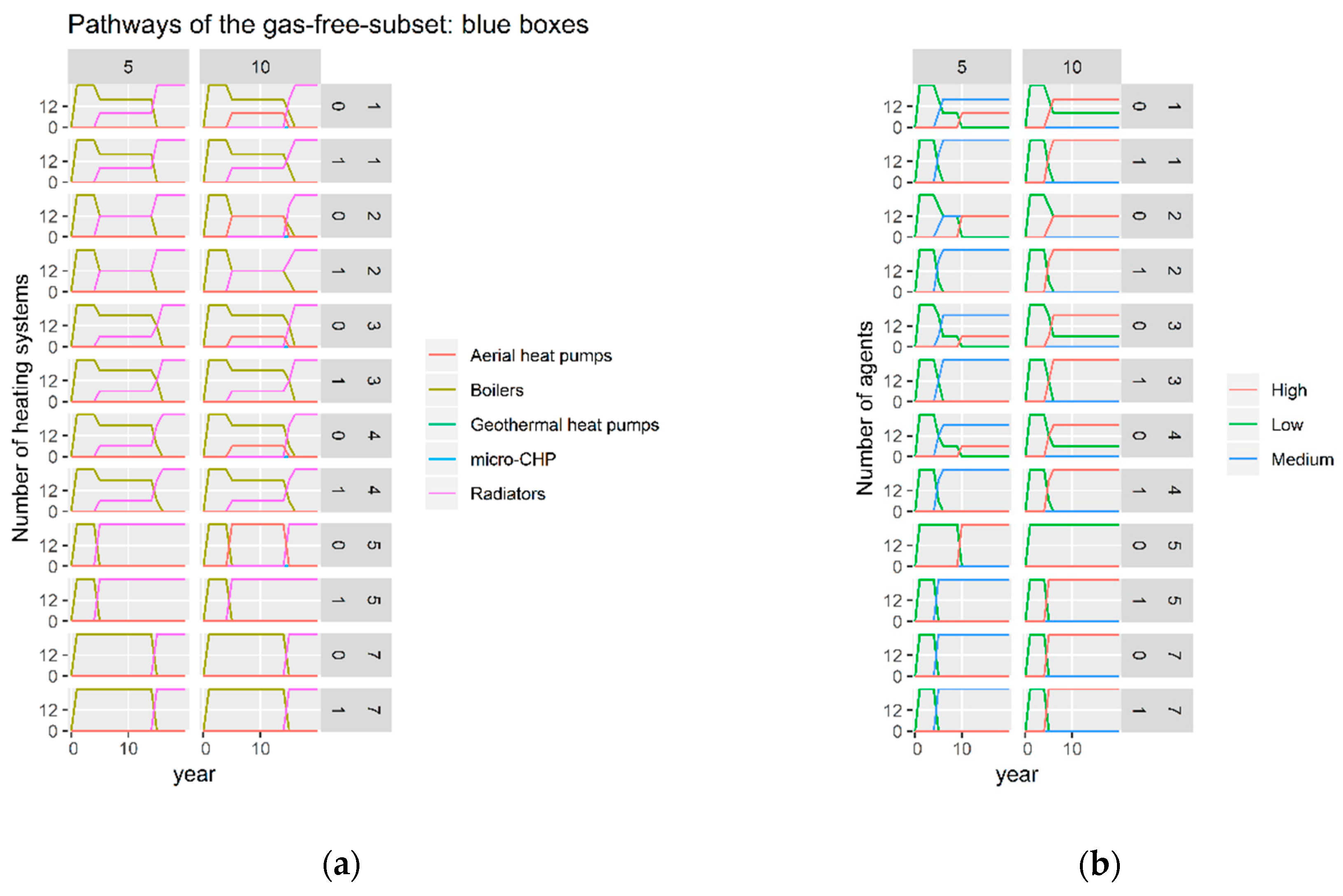
5.3. Modeling Question 3: Changes in Technology and Insulation
5.4. Integration and Discussion
6. Conclusions
Supplementary Materials
Author Contributions
Funding
Acknowledgments
Conflicts of Interest
Appendix A. Additional Description of the ABM, Based on the ODD Protocol
Appendix A.1. Design Concepts
- Basic principle: The neighborhood’s cumulative costs and annual natural gas consumption results from individual decisions of households to use and replace their technology. Those decisions are based on some of agents’ state variables and external factors.
- Emergence: The neighborhood’s cumulative costs, annual natural gas consumption, number of heating systems of each type, and insulation levels.
- Adaptation: While households use current retail energy prices to select the heating system and insulation level that best meets their objectives, their state variables HRZ, ORI, THR, and ACCI remain constant during a simulation run.
- Objectives: Households are either natural gas minimizers (environmentally oriented) or cumulative cost minimizers (financially and socially oriented). Socially-oriented agents act only if a fraction of their peers has acted.
- Learning/prediction: Households do not use learning mechanisms nor forecasting. They assume that the current retail energy prices will remain constant.
- Sensing: Households are assumed to know the present price of heating systems, insulation levels, electricity and natural gas, and the number of heating systems of each type, and insulation levels in the neighborhood by the end of the previous year.
- Interaction: Socially-oriented households consider replacing their heating systems or improving their insulation only when a fraction of their peers has also made changes.
- Stochasticity: While the model is initialized stochastically, all properties of households but one are assigned deterministically (value orientation: ORI). Therefore, households are identical except for their value orientation. As a result, stochastic initialization does not have an effect on model outcomes.
- Collectives: The model does not account for aggregations between households. An example of aggregation would be multiple households investing together in one heating system to meet their heat demand.
- Observation: The neighborhood’s cumulative costs, annual natural gas consumption, number of heating systems of each type, and insulation levels are the variables used for observing system level behavior.
Appendix A.2. Initialization
Appendix A.3. Input Data

| Parameter | Value | Source |
|---|---|---|
| Retail natural gas prices for the first year [Euro/kWh] | 0.08 | Based on [50] |
| Retail electricity prices for the first year [Euro/kWh] | 0.16 | Based on [51] |
| Parameter | Value for Each Type of Technology | Source |
|---|---|---|
| Thermal efficiency [dmnl] | 1, 0.60, 1, 2.6, 3.3 | Assumptions and [49] |
| Electrical efficiency [dmnl] | 0, 0.28, 0, 0, 0 | Assumptions and [49] |
| Capital costs [€/kW] | 0, 2100, 300, 1130, 1675 | Assumptions and [49] |
| Annual operation costs [€ per kw/year] | 11.18, 42, 10, 22.6, 33.5 | Assumptions and [49] |
| Parameter | Value for Each Level | Source |
|---|---|---|
| Capacity required from a technology to meet demand [kW] | 15, 8, 5 | Assumptions |
| Capital costs when dwellings have low level [€] | NA *, 5500, 10000 | Assumptions |
| Capital costs when dwellings have medium level [€] | NA *, NA *, 6000 | Assumptions |
| Heat demand [kWh] | 25000, 10000, 5000 | Assumptions |
References
- European Commission. Press Release: Towards a Smart, Efficient and Sustainable Heating and Cooling Sector. Available online: http://europa.eu/rapid/press-release_MEMO-16-311_ en.htm#_ftnref1 (accessed on 2 February 2019).
- Holtinnen, H.; Tuohy, A.; Milligan, M.; Lannoye, E.; Silva, V.; Müller, S.; Söder, L. The flexibility workout: Managing variable resources and assessing the need for power system modification. IEEE Power Energy Mag. 2013, 11, 53–62. [Google Scholar] [CrossRef]
- Mathiesen, B.V.; Lund, H.; Connolly, D.; Wenzel, H.; Østergaard, P.A.; Möller, B.; Nielsen, S.; Ridjan, I.; Karnøe, P.; Sperling, K.; et al. Smart Energy Systems for coherent 100% renewable energy and transport solutions. Appl. Energy 2015, 145, 139–154. [Google Scholar] [CrossRef]
- Lund, H.; Andersen, A.N.; Østergaard, P.A.; Mathiesen, B.V.; Connolly, D. From electricity smart grids to smart energy systems—A market operation based approach and understanding. Energy 2012, 42, 96–102. [Google Scholar] [CrossRef]
- Lund, H.; Werner, S.; Wiltshire, R.; Svendsen, S.; Thorsen, J.E.; Hvelplund, F.; Mathiesen, B.V. 4th Generation District Heating (4GDH). Energy 2014, 68, 1–11. [Google Scholar] [CrossRef]
- Herder, P.M.; Bouwmans, I.; Dijkema, G.P.J.; Stikkelman, R.M.; Weijnen, M.P.C. Designing Infrastructures from a Complex Systems Perspective. ResearchGate 2008, 7, 17–34. [Google Scholar]
- Moncada Escudero, J.A.; Nava Guerrero, G.D.C.; Park Lee, H.K.; Okur, Ö.; Chakraborty, S.T.; Lukszo, Z. Complex Systems Engineering: Designing in sociotechnical systems for the energy transition. EAI Endorsed Trans. Energy Web 2017, 17. [Google Scholar] [CrossRef]
- Cooper, R.; Foster, M. Sociotechnical systems. Am. Psychol. 1971, 26, 467–474. [Google Scholar] [CrossRef]
- Trist, E.L. The Evolution of Socio-Technical Systems: A Conceptual Framework and an Action Research Program; Ontario Ministry of Labour, Ontario Quality of Working Life Centre: Toronto, ON, Canada, 1981. [Google Scholar]
- Enserink, B.; Kwakkel, J.; Bots, P.; Hermans, L.; Thissen, W.; Koppenjan, J. Policy Analysis of Multi-Actor Systems; Eleven International Publishing: The Hague, The Netherlands, 2010. [Google Scholar]
- March, J.G. Bounded Rationality, Ambiguity, and the Engineering of Choice. Bell J. Econ. 1978, 9, 587–608. [Google Scholar] [CrossRef]
- Simon, H.A. Models of Bounded Rationality: Empirically Grounded Economic Reason; MIT Press: Cambridge, MA, USA, 1997. [Google Scholar]
- Bengtsson, M.; Kock, S. Cooperation and competition in relationships between competitors in business networks. J. Bus. Ind. Mark. 1999, 14, 178–194. [Google Scholar] [CrossRef]
- North, D.C. Institutions. J. Econ. Perspect. 1991, 5, 97–112. [Google Scholar] [CrossRef]
- Holland, J.H. The Global Economy as an Adaptive Process. In The Economy as an Evolving Complex System; CRC Press: Boca Raton, FL, USA, 1988. [Google Scholar]
- Waldorp, M. Complexity: The Emerging Science at the Edge of Order and Chaos; Simon and Schuster: New York, NY, USA, 1992. [Google Scholar]
- Grimm, V.; Railsback, S.F. Individual-Based Modeling and Ecology; Princeton University Press: Princeton, NJ, USA, 2004. [Google Scholar]
- Railsback, S.F.; Grimm, V. Agent-Based and Individual-Based Modeling: A Practical Introduction, 2nd ed.; Princeton University Press: Princeton, NJ, USA, 2019. [Google Scholar]
- North, M.J.; Macal, C.M. Managing Business Complexity: Discovering Strategic Solutions with Agent-Based Modeling and Simulation; Oxford University Press: Oxford, UK, 2007. [Google Scholar]
- Nikolic, I.; Kasmire, J. Theory. In Agent-Based Modelling of Socio-Technical Systems; van Dam, K.H., Nikolic, I., Lukszo, Z., Eds.; Agent-Based Social Systems; Springer Netherlands: Dordrecht, The Netherlands, 2013; pp. 11–71. [Google Scholar]
- Borshchev, A.; Filippov, A. From System Dynamics and Discrete Event to Practical Agent Based Modeling: Reasons, Techniques, Tools. In Proceedings of the 22nd international conference of the system dynamics society, Oxford, UK, 25–29 July 2004. [Google Scholar]
- van Dam, K. Capturing Socio-Technical Systems with Agent-Based Modelling. Ph.D. Thesis, Delft University of Technology, Delft, The Netherlands, 2009. [Google Scholar]
- Olivella-Rosell, P.; Villafafila-Robles, R.; Sumper, A.; Bergas-Jané, J. Probabilistic Agent-Based Model of Electric Vehicle Charging Demand to Analyse the Impact on Distribution Networks. Energies 2015, 8, 4160–4187. [Google Scholar] [CrossRef]
- Agent-Based Modelling of Socio-Technical Systems; van Dam, K.H., Nikolic, I., Lukszo, Z., Eds.; Agent-Based Social Systems; Springer Netherlands: Dordrecht, The Netherlands, 2013. [Google Scholar]
- Jennings, N.R. On agent-based software engineering. Artif. Intell. 2000, 117, 277–296. [Google Scholar] [CrossRef]
- Wooldridge, M.; Jennings, N.R. Intelligent agents: Theory and practice. Knowl. Eng. Rev. 1995, 10, 115. [Google Scholar] [CrossRef]
- Holland, J.H. Hidden Order: How Adaptation Builds Complexity; Addison-Wesley: New York, NY, USA, 1995. [Google Scholar]
- Nikolic, I. Co-Evolutionary Method for Modelling Large Scale Socio-Technical Systems Evolution. Ph.D. Thesis, Delft University of Technology, Delft, The Netherlands, 2009. [Google Scholar]
- Companion Modelling: A Participatory Approach to Support Sustainable Development; Etienne, M., Ed.; Springer: Dordrecht, The Netherlands, 2014. [Google Scholar]
- Vespignani, A. Modelling dynamical processes in complex socio-technical systems. Nat. Phys. 2012, 8, 32–39. [Google Scholar] [CrossRef]
- Li, F.G.N.; Trutnevyte, E.; Strachan, N. A review of socio-technical energy transition (STET) models. Technol. Forecast. Soc. Chang. 2015, 100, 290–305. [Google Scholar] [CrossRef]
- Hesselink, L.X.W.; Chappin, E.J.L. Adoption of energy efficient technologies by households–Barriers, policies and agent-based modelling studies. Renew. Sustain. Energy Rev. 2019, 99, 29–41. [Google Scholar] [CrossRef]
- Grimm, V.; Berger, U.; DeAngelis, D.L.; Polhill, J.G.; Giske, J.; Railsback, S.F. The ODD protocol: A review and first update. Ecol. Model. 2010, 221, 2760–2768. [Google Scholar] [CrossRef]
- Wilensky, U. Center for Connected Learning and Computer-Based Modeling; Northwestern University: Evanston, IL, USA, 1999. [Google Scholar]
- Grignard, A.; Taillandier, P.; Gaudou, B.; Vo, D.A.; Huynh, N.Q.; Drogoul, A. GAMA 1.6: Advancing the Art of Complex Agent-Based Modeling and Simulation. In PRIMA 2013: Principles and Practice of Multi-Agent Systems; Boella, G., Elkind, E., Savarimuthu, B.T.R., Dignum, F., Purvis, M.K., Eds.; Springer: Berlin/Heidelberg, Germany, 2013; pp. 117–131. [Google Scholar]
- Sklar, E. NetLogo, a Multi-agent Simulation Environment. Artif. Life 2007, 13, 303–311. [Google Scholar] [CrossRef] [PubMed]
- R Core Team. R: A Language and Environment for Statistical Computing; R Foundation for Statistical Computing: Vienna, Austria, 2018. [Google Scholar]
- RStudio. RStudio: Integrated Development Environment for R; RStudio: Boston, MA, USA, 2018. [Google Scholar]
- Wickham, H.; François, R.; Henry, L.; Müller, K. dplyr: A Grammar of Data Manipulation; 2019. Available online: https://CRAN.R-project.org/package=dplyr (accessed on 1 March 2019).
- Grothendieck, G. SQLDF: Manipulate R Data Frames Using SQL; 2017. Available online: https://CRAN.R-project.org/package=sqldf (accessed on 1 March 2019).
- Wickham, H.; Chang, W.; Henry, L.; Pedersen, T.L.; Takahashi, K.; Wilke, C.; Woo, K. ggplot2: Create Elegant Data Visualisations Using the Grammar of Graphics; 2018. Available online: https://CRAN.R-project.org/package=ggplot2 (accessed on 1 March 2019).
- Fox, J.; Weisberg, S.; Price, B.; Adler, D.; Bates, D.; Baud-Bovy, G.; Bolker, B.; Ellison, S.; Firth, D.; Friendly, M.; et al. CAR: Companion to Applied Regression; 2018. Available online: https://CRAN.R-project.org/package=car (accessed on 1 March 2019).
- Beurskens, L.W.M.; Menkveld, M. Renewable heating and cooling in the Netherlands. D3 of WP2 from the RES-H Policy project. In Duurzame Warmte en Koude in Nederland. D3 van WP2 van het RES-H Policy Project; Energieonderzoek Centrum Nederland (ECN): Petten, The Netherlands, 2009. [Google Scholar]
- Ministerie van Economische Zaken en Klimaat Kamerbrief over Gaswinning Groningen-Kamerstuk-Rijksoverheid.nl. Available online: https://www.rijksoverheid.nl/documenten/kamerstukken/2018/03/29/kamerbrief-over-gaswinning-groningen (accessed on 4 February 2019).
- The Groningen Gas Field. Available online: http://www.geoexpro.com/articles/2009/04/the-groningen-gas-field (accessed on 10 February 2019).
- Aardgasvrij|RVO.nl. Available online: https://www.rvo.nl/onderwerpen/duurzaam-ondernemen/duurzame-energie-opwekken/aardgasvrij (accessed on 20 February 2019).
- Ministerie van Economische Zaken; Ministerie van Infrastructuur en Energieagenda: Naar een CO2-Arme Energievoorziening-Rapport-Rijksoverheid.nl. Available online: https://www.rijksoverheid.nl/documenten/rapporten/2016/12/07/ea (accessed on 4 February 2019).
- Technology Data for Energy Plants. Individual Heating Plants and Energy Transport (Technical Report)|ETDEWEB. Available online: https://www.osti.gov/etdeweb/biblio/1049406 (accessed on 19 February 2019).
- Fleiter, T.; Steinbach, J.; Ragwitz, M.; Arens, M.; Aydemir, A.; Elsland, R.; Naegeli, C. Mapping and analyses of the current and future (2020–2030) heating/cooling fuel deployment (fossil/renewables). Work Package 2: Assessment of the Technologies for the Year 2012. 2016. Available online: https://ec.europa.eu/energy/sites/ener/files/documents/mapping-hc-final_report-wp2.pdf (accessed on 1 March 2019).
- Eurostat Gas Prices by Type of User. Available online: https://ec.europa.eu/eurostat/tgm/table.do?tab=table&init=1&language=en&pcode=ten00118&plugin=1 (accessed on 2 February 2019).
- Eurostat. Electricity Prices by Type of User. Available online: https://ec.europa.eu/eurostat/tgm/table.do?tab=table&init=1&language=en&pcode=ten00117&plugin=1 (accessed on 2 February 2019).


| Variable | Units | Description | Possible Values |
|---|---|---|---|
| Insulation level | Dimensionless | Insulation level of a dwelling | Low, Medium or High |
| Heating system | Dimensionless | Type of heating system | Natural gas boiler, electric radiator, micro-CHP, aerial heat pump, geothermal heat pump |
| Annual natural gas consumption | [MWh] | Gas consumption in one year | Positive real numbers |
| Cumulative costs | Thousands of Euros | Investment, maintenance and operation costs | Positive real numbers |
| HRZ | Years | Time horizon | Positive integers |
| INV | Years | Indicates the number of years left before a time equal to the agent’s HRZ has passed since the agent’s last investment | Positive integers |
| ORI | Dimensionless | Value orientation | Environmental, Social, Financial |
| THR | Dimensionless | Threshold after which socially oriented agents will make a decision | 0 ≤ Fraction ≤ 1 |
| ACCI | Dimensionless | Ability to compare combined investments | 0 ≤ Fraction ≤ 1 |
| Variable | Units | Description | Possible Values |
|---|---|---|---|
| dgp | %/year | Annual percentage change in the retail natural gas price | Real numbers |
| dep | %/year | Annual percentage change in the retail electricity price | Real numbers |
| popACCI | Dimensionless | Fraction of households in the population that is able to compare combined investments. | 0 ≤ Fraction ≤ 1 |
| popHRZ | Dimensionless | Time horizon shared by all households in the population, in years. | Positive integers |
| popORI | Dimensionless | Fraction of households in the population with each value orientation: Environmental (Env), social (Soc) and financial (Fin). | 0 ≤ Env, Soc, Fin ≤ 1 [Env, Soc, Fin] Env + Soc + Fin = 1 |
| Type of Variation | Groups of Variations |
|---|---|
| dgp | −0.04, 0, 0.04 |
| dep | −0.04, 0, 0.04 |
| popORI | 1 = [0.33, 0.33, 0.33] 2 = [0.50, 0.25, 0.25] 3 = [0.25, 0.50, 0.25] 4 = [0.25, 0.25, 0.50] 5 = [1, 0, 0] 6 = [0, 1, 0] 7 = [0, 0, 1] |
| popACCI | 0 and 1 |
| popHRZ | 1, 5, 10, 15, 20, 30 |
| Subset | Number of Scenarios | Definition |
|---|---|---|
| All-simulation-runs | 756 | Results from all simulation runs. |
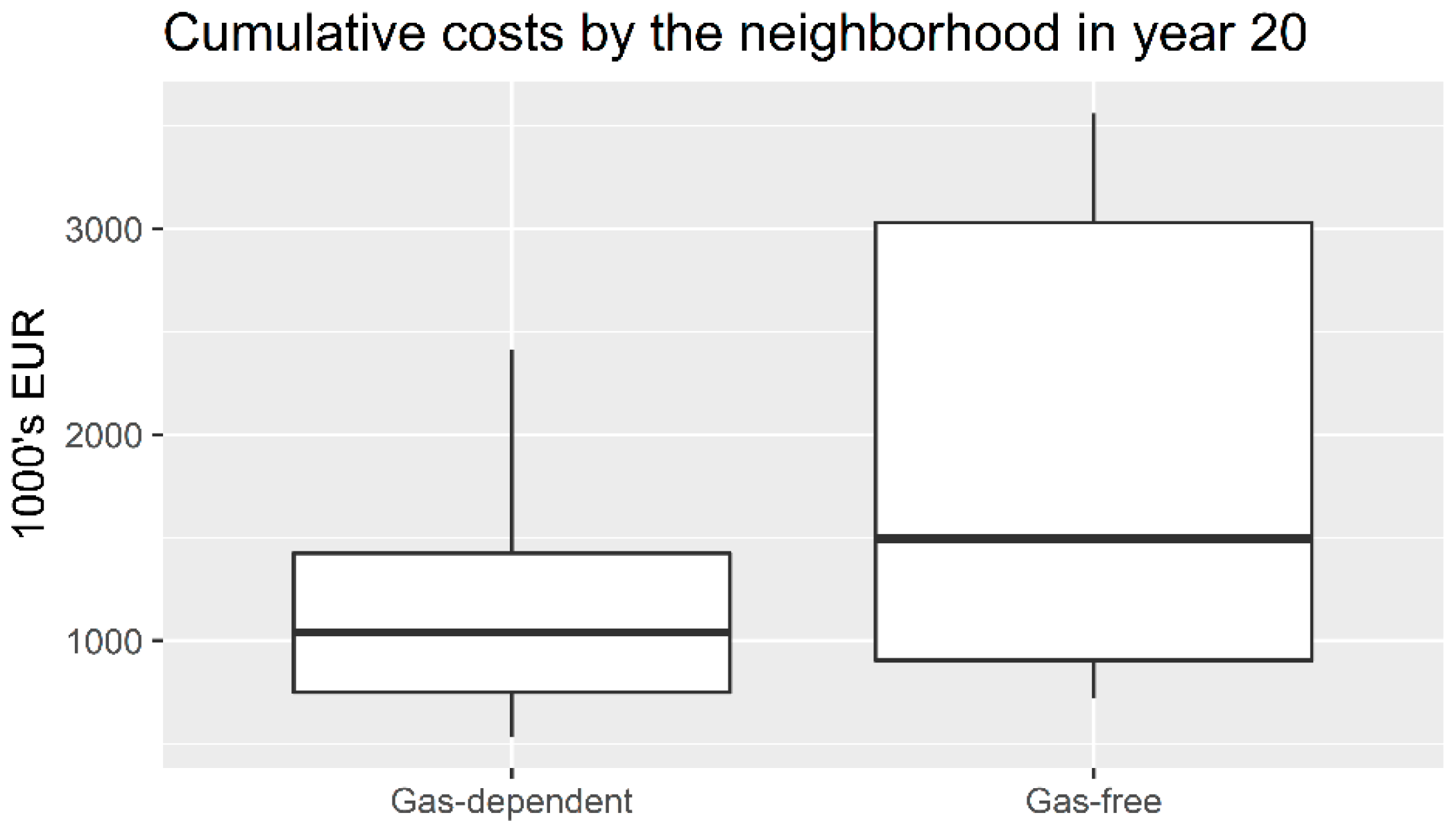
| Gas-dependent-subset | 628 | Subset of all-simulation-runs in which the neighborhood consumed natural gas in year 20, and thus did not achieve the transition to a gas-free neighborhood. |
| Gas-free-subset | 128 | Subset of all-simulation-runs in which did not consume natural gas in year 20, and thus fully achieved the thermal energy transition to a gas-free neighborhood. |
| Type of Variation | Set 1 | Set 2 |
|---|---|---|
| popORI | 5 | 1, 2, 3, 4, 7 |
| popHRZ | - | 5, 10 |
| dgp | - | increasing |
| dep | - | decreasing |
| Group | Number of Scenarios | Mean | Standard Deviation | Median | IQR * |
|---|---|---|---|---|---|
| All-simulation-runs | 756 | 1238 | 640 | 1040 | 760 |
| Gas-dependent-subset | 628 | 1105 | 420 | 1040 | 676 |
| Gas-free-subset | 128 | 1889 | 1027 | 1495 | 2126 |
| Test | Results | Conclusion |
|---|---|---|
| Wilcoxon rank sum test | W = 22403 p-value = 2.745e-15 | Groups’ medians are significantly different |
| Shapiro-Wilk normality test | W = 0.96395 p-value = 1.077e-12 | Sample deviates from normality |
© 2019 by the authors. Licensee MDPI, Basel, Switzerland. This article is an open access article distributed under the terms and conditions of the Creative Commons Attribution (CC BY) license (http://creativecommons.org/licenses/by/4.0/).
Share and Cite
Nava Guerrero, G.d.C.; Korevaar, G.; Hansen, H.H.; Lukszo, Z. Agent-Based Modeling of a Thermal Energy Transition in the Built Environment. Energies 2019, 12, 856. https://doi.org/10.3390/en12050856
Nava Guerrero GdC, Korevaar G, Hansen HH, Lukszo Z. Agent-Based Modeling of a Thermal Energy Transition in the Built Environment. Energies. 2019; 12(5):856. https://doi.org/10.3390/en12050856
Chicago/Turabian StyleNava Guerrero, Graciela del Carmen, Gijsbert Korevaar, Helle Hvid Hansen, and Zofia Lukszo. 2019. "Agent-Based Modeling of a Thermal Energy Transition in the Built Environment" Energies 12, no. 5: 856. https://doi.org/10.3390/en12050856
APA StyleNava Guerrero, G. d. C., Korevaar, G., Hansen, H. H., & Lukszo, Z. (2019). Agent-Based Modeling of a Thermal Energy Transition in the Built Environment. Energies, 12(5), 856. https://doi.org/10.3390/en12050856