Determining Soil-Water Characteristic Curves from Mercury Intrusion Porosimeter Test Data Using Fractal Theory

Abstract

Accurate determination of soil-water characteristic curve (SWCC) is of immense importance for understanding the mechanical behavior of unsaturated soils. Due to the difficulty and long duration of experimental procedures, it is of great significance to estimate the SWCC by indirect methods. To address this issue, in this article an effective fractal method is proposed for predicting the SWCC based on mercury intrusion porosimeter (MIP) data. Only two characteristic parameters, namely the fractal dimension and air-entry value, are needed in the presented approach. Detailed procedures for determining the parameters are clearly elaborated. Due to the influence of sample size difference on the equivalent connected pore size, a sample scale effect coefficient is proposed to predict air-entry values. The concept of “critical pore size” is introduced to obtain the optimal fractal dimension, which can accurately reflect the fractal behaviour of SWCC samples. By comparisons between predicted and experimental SWCCs, the validation of the proposed method is verified. The comparisons reveal the good agreement between the proposed approach and laboratory experiments.

1. Introduction

Accurate determination of soil-water characteristic curves (SWCCs) is crucial to understand the shear strength, permeability coefficient, volume strain and water distribution of unsaturated soils. Due to the difficulty and long duration of experimental procedures, over the past years, increasing efforts have been focused on indirect estimations of SWCCs.

In recent years, various attempts have been made to predict SWCC from the pore size distribution (PSD) [1,2,3,4]. For a given state of soils, it has been reported that PSD has great influence on SWCC [5,6]. However, the soil structure pores feature large numbers of different complex shapes, which are difficult to described using classical geometry.

Fractal theory has been increasingly recognized as a valid approach for describing the complex structures of geomaterials [7,8,9,10,11]. Ghanbarian and Hunt [12] in particular have stressed the application of fractal theory to geomaterials. As a result, by employing fractal theory, various attempts have been made to relate SWCC with PSD. For example, Tyler and Wheatcraft [13] simulated the PSD of soils by using a Sierpinski carpet, and derived a SWCC expression with the Sierpinski carpet structure. Perrier et al. [14] and Xu et al. [15,16] proposed SWCC models employing a fractal model of the pore volume distribution, which was developed on the basis of Mandelbrot’s model expressing the relationship between volume and quantity distribution of fractal matter. Many contributions rely on the pore-solid fractal model to establish fractal SWCC models of PSD [17,18,19,20]. Ghanbarian-Alavijeh and Millan [21] researched the relationship between surface fractal dimensions derived from SWCC and water content remaining at high tensions as well as clay content. In addition, Ghanbarian-Alavijeh et al. [22] proposed a comprehensive review of various fractal SWCC models, and pointed out the advantages and disadvantages of the various models. Although various fractal SWCC models have been established, the determination of the parameters used in those models is not an easy task. In addition, most of them have failed to verify the rationality of the model using pore tests and SWCC tests at the same time. As a result, the approach of predicting SWCC from PSD is mainly in a stage of model research, and an effective method has not been formed yet. In this respect, Tao et al. [23] fortunately proposed a fractal approach to predict SWCC from Nuclear Magnetic Resonance (NMR) test data, and conducted both NMR and SWCC tests to verify the accuracy of their approach.

On the other hand, many techniques are able to quantitatively determine the PSD of soil, such as digital image technology, CT technology, mercury intrusion porosimeter (MIP), etc. [24,25,26,27]. Among them, the MIP technique can easily obtain the distribution law of soil pores, so it has been widely used in the research of pore structures of geotechnical materials. Based on capillary theory, it is theoretically feasible to predict SWCC from MIP technique data, unfortunately, its accuracy for predicting SWCC using the original Young-Laplace equation is not sufficient [28,29,30,31,32,33]. An important difference between MIP tests and SWCC is the size of the test samples, which has an influence on the prediction accuracy of SWCC, but this was usually ignored in prior studies.

To solve this issue, a new prediction approach for SWCC is presented herein, in which the MIP technique is employed to determine two parameters, namely fractal dimension and air-entry value. Considering sample size differences, a sample scale effect coefficient is introduced to predict the air-entry value, which greatly improves the accuracy of the predicted SWCC. The concept of “critical pore size” is further introduced to obtain the optimal fractal dimensions. The accuracy of the proposed approach is thoroughly verified through the experimental data from MIP and SWCC tests.

2. MIP Theory

In the MIP test, a non-wetting fluid (mercury) is employed to penetrate the voids of a porous material under increasing absolute pressures. Due to the influence of surface tension, the mercury must be subjected to a certain external pressure when it enters a small pore, so the volume of intruded mercury is the volume of the pore. The theoretical relationship between the intrusion pressure p and the pore diameter d can be described by the Young-Laplace equation:

$$p=-\frac{4T_m\cos {\theta }_m}{d}$$

(1)

where T_m is the surface tension of mercury; θ_m is the contact angle between mercury and soil interface.

For water, the same relation applies:

$$\psi =\frac{4T_s\cos \alpha }{d}$$

(2)

in which, Ψ, T_s and α are the corresponding parameters for water.

Dividing Equation (1) by Equation (2) gives:

$$\psi =-\frac{T_s\cos \alpha }{T_m\cos {\theta }_m}p$$

(3)

Regarding applications from Equations (1) and (2), the mercury pressure and the matrix suction have a one-to-one correspondence with the pore diameter. Mercury invades pores with a diameter of more than d firstly, so there is S_Hg = V(≥d)/V, where S_Hg is the degree of saturation of mercury, V(≥d) is the volume of pore diameter greater than d, V is the volume of sample. However, under the action of matrix suction corresponding to the same pore diameter d, water enters pores with a diameter less than d firstly, so there is S_w = V(≤d)/V, where S_w is the degree of saturation of water, V(≤d) is the volume of pore diameter less than d. Assuming that all soil pores are filled with liquid (mercury or water), then we have:

$$S_w+S_{Hg}=1$$

(4)

Based on this theory, SWCC can be predicted from MIP test results. There are nevertheless some fundamental differences between the SWCC and the MIP test. For the MIP test, the interface medium is a non-wetting liquid (mercury), whereas for SWCC test, the interface medium is a wetting liquid (water), as shown in Figure 1. In addition, the sample size of MIP tests is very different from that of a SWCC test, which results in the fact that the porosity and PSD of a MIP test sample cannot reliably reflect those of a SWCC test sample. Consequently, the prior works show that it is not ideal to directly predict the SWCC from MIP test results [28,29,30,31,32,33].

To solve this issue, a new SWCC fractal model is presented in following section, where the MIP test only serves as a basis to determine the parameters of the model.

3. SWCC Fractal Model

Following Zhang et al. [34], a porosity model is expressed as:

$$\phi (>d)=1-{(\frac{d}{d_{max}^{}})}^{3-D}$$

(5)

where d_max is the maximum characteristic pore size, d_min is the minimum characteristic pore size, D is fractal dimension, φ(>d) is the porosity of pore size greater than d. If d is equal to d_min, total porosity φ is described as:

$$\phi =1-{(\frac{d_{\min }^{}}{d_{max}^{}})}^{3-D}$$

(6)

If the volumetric water content is expressed by θ, then θ = φ(≤d) = φ −φ(>d). Substituting θ into Equation (6) gives:

$$\theta =\phi -1+{(\frac{d}{d_{max}})}^{3-D}$$

(7)

The matrix suction Ψ corresponding to d_max represents the air-entry value Ψ_a, which is obtained from Equation (2):

$${\psi }_a=\frac{4T_s\cos \alpha }{d_{max}}$$

(8)

Considering Equations (2), (7) and (8), Equation can be rewritten as:

$$\theta =\phi -1+{(\frac{{\psi }_a}{\psi })}^{3-D}$$

(9)

Interestingly, it is noted that the above proposed model is exactly consistent with the hypothetical aggregate model established by Rieu and Sposito [35].

Equation (9) is a SWCC model as presented in terms of the volumetric water content θ. By using the basic relationship between θ and w, Equation (9) can be converted to:

$$w=\frac{(1+e){({\psi }_a/\psi )}^{3-D}-1}{G_s}$$

(10)

where G_s is the relative density of a particle, e is the void ratio. We note that Equation (10) takes effect at the stage when Ψ > Ψ_a, while w is approximately assumed to be equal to the saturated gravimetric water content at the stage when Ψ ≤ Ψ_a, namely w = e/G_s.

Regarding applications of Equation (10), the SWCC is controlled by D and Ψ_a (Figure 2). D is linked to the shape of SWCC, and Ψ_a. has influence on the starting point of SWCC. The fractal dimensions have an obvious relationship with the clay content of soil [19,21]. The higher the clay content is, the smaller the fractal dimension is. In general, the fractal dimension of a sandy soil is far less than that of a clay soil. For a sandy soil, its water content can reach the residual water content when the matrix suction is low. In this paper, residual water content is seen as a part of the soil particles, therefore its value approaches to zero.

To predict the SWCC, the core problem in the next section will be to focus on accurately predicting D and Ψ_a for a given G_s and e.

4. Parameter Determination from MIP Test Results

4.1. Fractal Dimension

Assuming the total volume of a soil sample is taken as one, Equation (7) is rewritten as:

$${(\frac{d}{d_{max}})}^{3-D}=1-\phi +V(\le d)$$

(11)

Applying logarithms on both sides of Equation (11) yields:

$$(3-D)\ln d\propto \ln (1-\phi +V(\le d))$$

(12)

By plotting the lnd against ln(1 – φ + V(≤d)), D is then obtained by linear fitting to the MIP test data.

4.2. Air-Entry Value

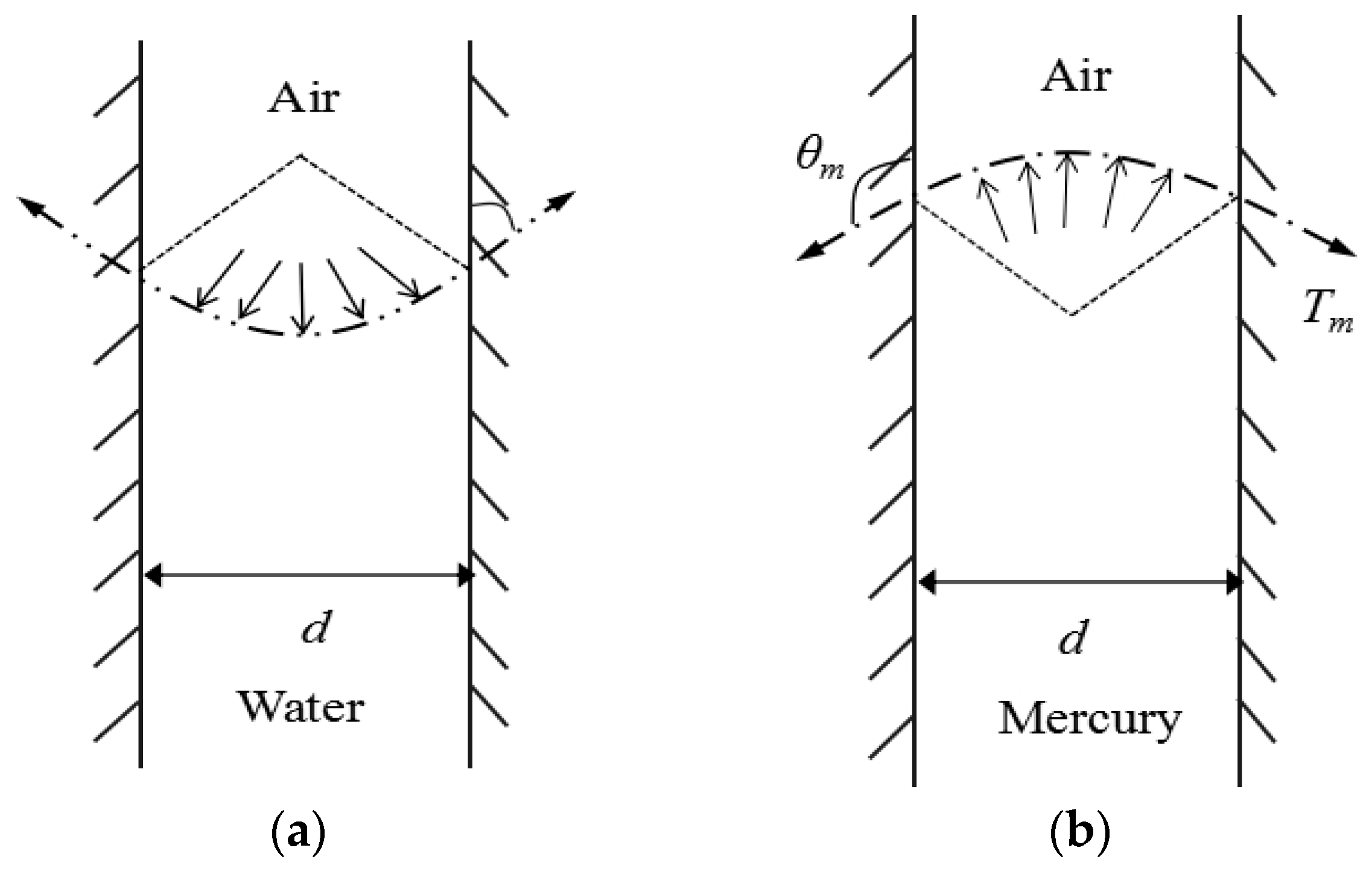
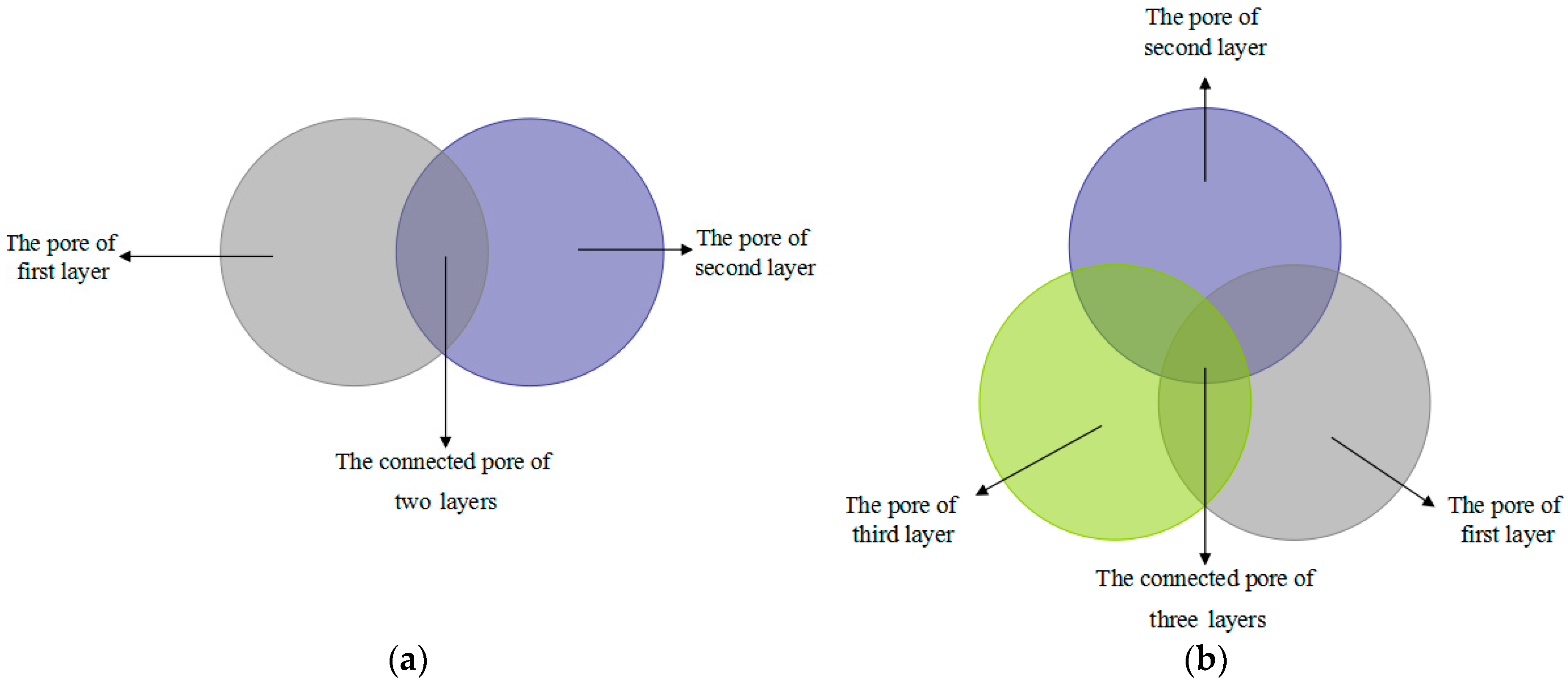
4.2.1. Sample Scale Effect

The volume of a MIP test sample is around 1 cm³, while that of a pressure plate test sample is 60 cm³, indicating that the size of the two test samples are very different. In Equation (2), d is the equivalent connected pore size. For a given soil sample, a change of sample size will induce a change of the equivalent connected pore size. If samples are regarded as several pieces of thin-layer soil, the equivalent connected pore size of a single slice of sample will be different from that of a sample with n superimposed layers. Figure 3 shows the relevant schematic diagram, where it can be seen that for a specific pore, the equivalent connected pore size diminishes with the increment of thickness of the layer. A parameter λ is introduced to consider the sample scale effect, that is to say, the equivalent connected pore size of MIP test sample is d, while that of pressure plate test sample will be λd (λ < 1).

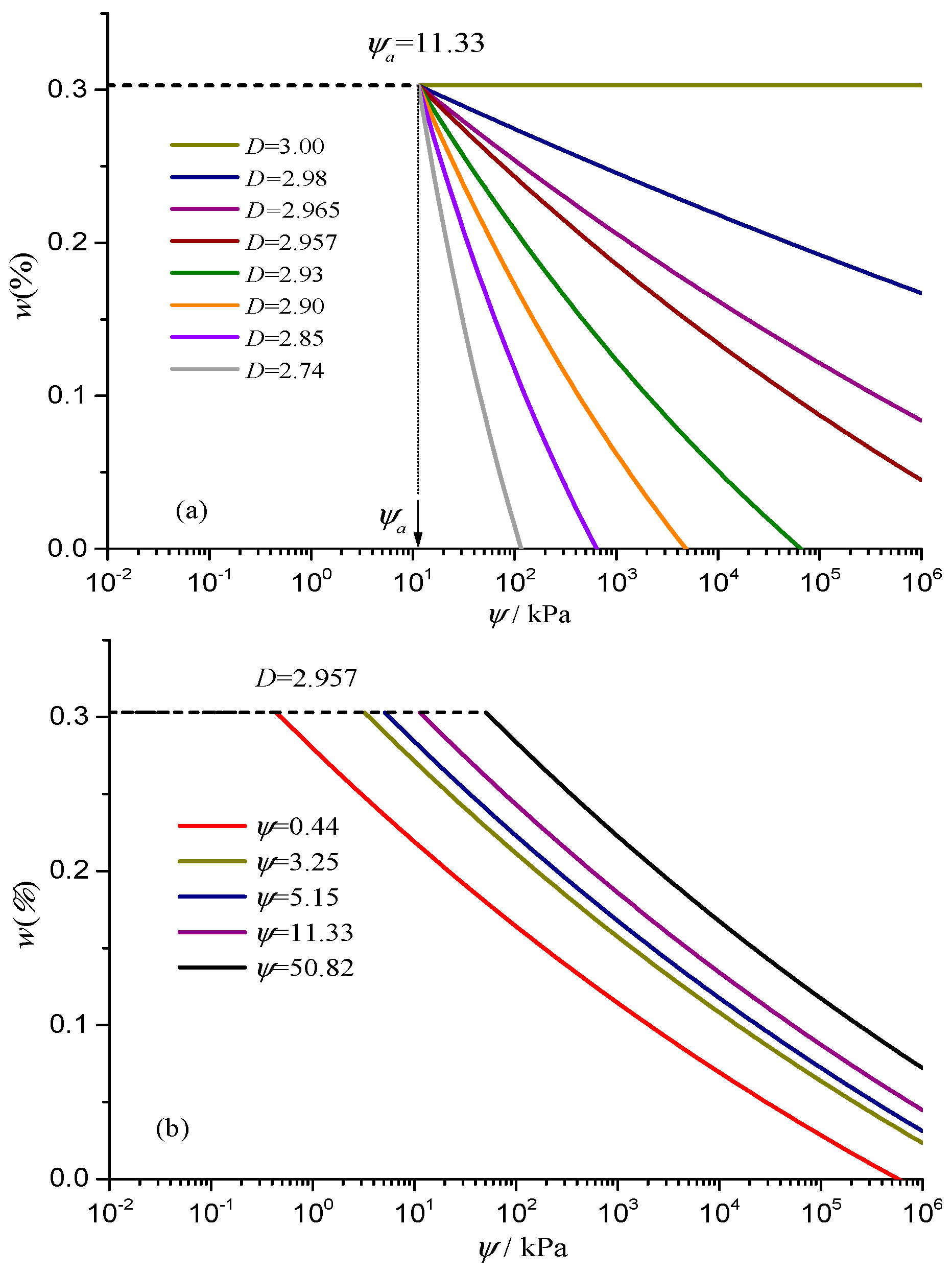
4.2.2. Determining the Air-Entry Value Ψ_a by Considering the Sample Scale Effect

Considering the sample scale effect, Equation (2) can be rewritten as:

$$\psi =\frac{4T_s\cos \alpha }{\lambda d}$$

(13)

so, the air-entry value is determined by:

$${\psi }_a=\frac{4T_s\cos \alpha }{\lambda d_{max}}$$

(14)

where the sample scale effect coefficient λ is taken as 0.1, 4T_scosα is equal to 300 μN/m (in which T_s is seen as 72.75 μN/m at the room temperature, and the contact angle is generally about 0°). Therefore, the core problem is the determination of maximum characteristic pore size d_max. Here, d_max is captured by Equation (6), where D is determined from MIP test data. The total porosity of samples is easily obtained, so the key point is to obtain the minimum characteristic pore size d_min. The total porosity can be obtained by the “oven-drying” method, in which the sample is dried at a constant temperature in the range of 100–105 °C, that is to say, the minimum pore size dried in the range of 100–105 °C should be taken account to determine d_min. As demonstrated by Tan et al. [36] and Zhao et al. [37], water in the soil is divided into liquid water, solid water and vapor water. The amount of vapor water can be ignored herewith, so the water in the soil mainly consists of solid water and liquid water.

Furthermore, liquid water is divided into free and bound water, where the free water consists of gravity and capillary water. The gravity water can move by its own gravity, while the capillary water is subjected to a surface tension force whose influence area approximately ranges from 1 nm to 10⁴ nm; the bound water is subjected to van der Waals forces, whose influence area approximately ranges from 0.3 nm to 10² nm. During the process of oven-drying at constant temperature, all liquid water of soil almost evaporates, so the minimum characteristic pore size d_min is not more than 0.3 nm. The solid water is influenced by hydrogen and covalent bonds, whose influence area approximately ranges from 0.2 nm to 0.3 nm and 0.1 nm to 0.2 nm, respectively. During the process of oven-drying, part of the solid water evaporates, but another part still remains in the soil sample. In other words, the range of minimum characteristic pore size is about from 0.1 nm to 0.3 nm, and here d_min is taken as 0.2 nm to predict the maximum characteristic pore size.

5. Materials and Tests

5.1. MIP Tests

The soil sample employed is a Wuhan clay soil, whose liquid limit is 38.9%, plastic limit of 20.4% and relative density is 2.75. For the preparation of test samples, the soil was air-dried until its water content showed little change. Then, the dried soil was crushed and passed through a 2 mm sieve. Subsequently, some distilled water was mixed with the dried soil to reach a certain water content. Importantly, the mixture needed to be put in a sealed box for at least 2 days, which makes the water distribute uniformly in the soil. Seven samples with different initial dry densities (1.30, 1.35, 1.40, 1.45, 1.45, 1.50, 1.60 and 1.71 g/cm³) were formed by using a hydraulic jack. After vacuum saturation, these samples were freeze-dried by liquid nitrogen, and then were cut into pieces of approximately 10 × 10 × 10 mm (length × width × height) with a sharp knife. The MIP test was performed by a professional operator using a PoreMaster33 instrument (Quantachrome, 1900 Corporate Drive Boynton Beach, FL 33426 USA).

5.2. SWCC Tests

The soil type and sample preparation are the same as the MIP test, but each SWCC test sample had a diameter of 61.8 mm and 20 mm in height. The samples after vacuum saturation were used for SWCC experiments using a soil moisture pressure plate, which mainly consists of a pressure cell, a high air entry (HAE) ceramic disc and a piezometer. The samples were placed on the HAE ceramic disc, the lower part of which is connected to a burette of water under atmospheric pressure. Air pressure was applied from 0 to 1250 kPa in several steps. When the weight of the burette becomes stable, the next pressure level is applied. During the experimental process the weight of the burette is recorded.

6. Results and Discussion

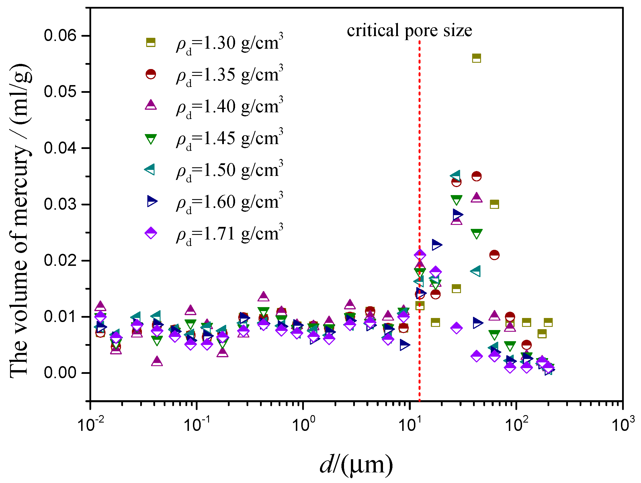
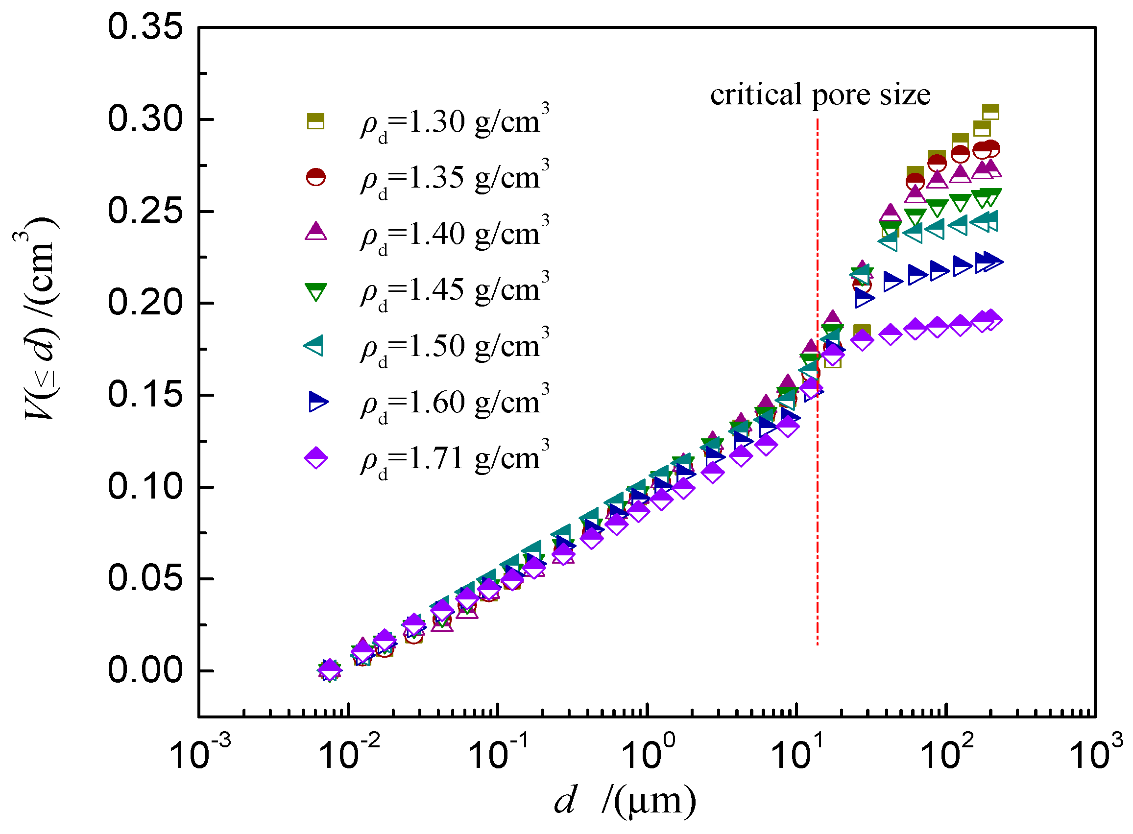
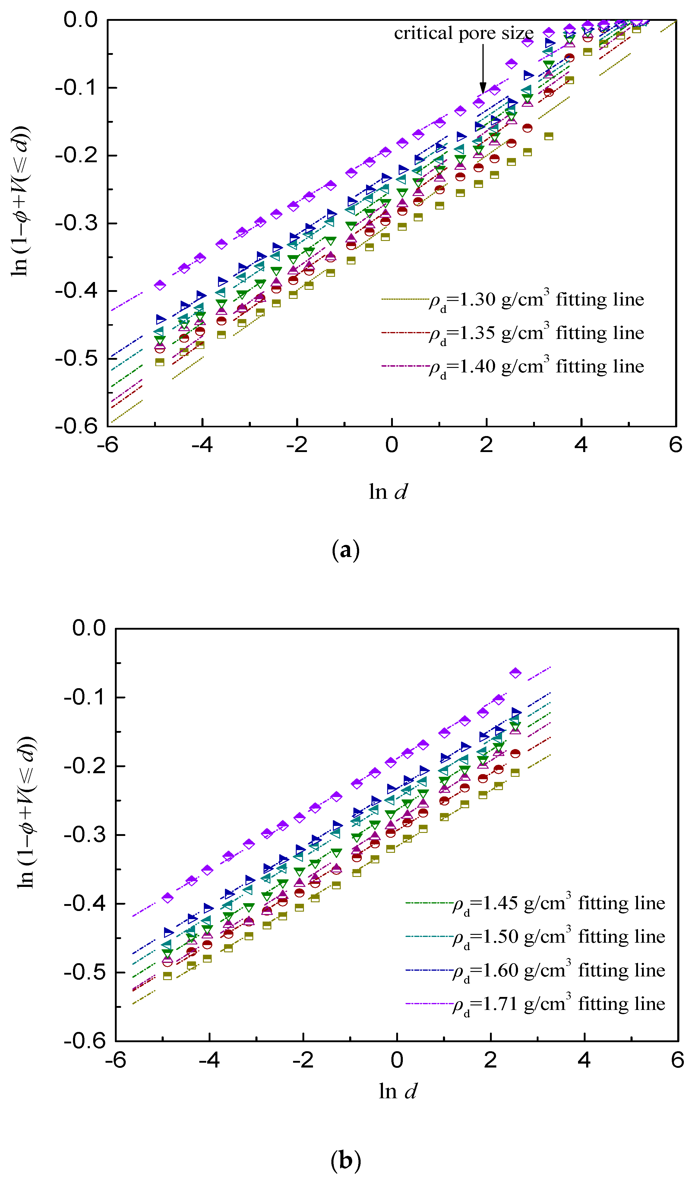
6.1. Critical Pore Size and Fractal Dimension

Figure 4 shows the PSD curves on the samples with different dry densities corresponding to a soil particle weighing 1 g.

In Figure 4, the PSD curves of samples with different dry densities are roughly similar in shape. For pores with diameters less than 12.5 μm, the PSD of different dry densities are almost undistinguishable, but for the pores with diameters beyond 12.5 μm, the PSD of different dry densities have great differences. This critical value (d = 12.5 μm) is denoted as the “critical pore size” d_c. Here, the pores with size beyond d_c are called “large pores”, while the pores with size less than d_c are called “small pores”. Consequently, small pores have stable properties, which are not affected by the dry density, while the properties of large pores are very unstable, and easily affected by the dry density.

The cumulative pore volume curves of different dry densities are shown in Figure 5, where it is found that the cumulative pore volume curves of different dry densities almost overlap when d is less than d_c, but when d increases to d_c, the cumulative curves of different dry densities have obvious differences. In addition, the experimental data less than d_c is distributed linearly, but this linear distribution disappears when the data is more than d_c. That is because that linear distribution of cumulative curves represents the good fractal behavior of soil. As presented by Tao et al. [38], the small pores have obvious fractal behavior, so the corresponding curves show a good linear distribution, however, the existence of large pores weakens the fractal behavior of pores, which results in that the corresponding pore size region shows an obvious nonlinear distribution.

Following the procedure presented in the above section, D is directly determined from fitting the experimental data to Equation (12), as shown in Figure 6a. The corresponding fitting linear expressions, correlation coefficient and the fractal dimension of unsaturated soil are shown in

Table 1. Fitting results of fractal dimension corresponding to Figure 6a.

Dry Density (g/cm3)	Expression of Fitting Line	Correlation Coefficient R2	Fractal Dimension D
1.30	y = 0.050x − 0.299	0.985	2.950
1.35	y = 0.050x − 0.276	0.989	2.950
1.40	y = 0.050x − 0.265	0.991	2.950
1.45	y = 0.049x − 0.251	0.994	2.951
1.50	y = 0.047x − 0.237	0.994	2.953
1.60	y = 0.046x − 0.225	0.995	2.954
1.71	y = 0.041x − 0.187	0.994	2.959

. It is found that the correlation coefficient is very high (>0.98) for all the experimental data, indicating that the fractal behaviour of the pores is significant.

In particular, it can be observed from Figure 6a that there exists a “turning point”, which is the abovementioned “critical pore size”. The experimental data less than d_c is distributed linearly, highlighting a more obvious fractal behavior. That is because that the PSD measured by MIP tests cannot fully reflect the essential characteristics of the original SWCC sample. The pores with size more than d_c are very unstable, and are greatly influenced by the density and size of soil sample, so their fractal characteristics are not obvious, while, the pores with size less than d_c are very stable, and are almost independent of the density and size of the soil sample, so their fractal characteristics are very strong. Due to the great difference in sample size between the MIP test and SWCC test, the fractal dimension obtained from the pore size data less than d_c can better reflect the fractal characteristics of the original pore structure of the SWCC sample.

Considering “critical pore size”, the prediction fractal dimensions are given in Figure 6b. Upon inspection of

Table 2. Fitting results of fractal dimension corresponding to Figure 6b.

Dry Density (g/cm3)	Expression of Fitting Line	Correlation Coefficient R2	Fractal Dimension D
1.30	y = 0.041x − 0.316	0.998	2.959
1.35	y = 0.041x − 0.293	0.998	2.959
1.40	y = 0.044x − 0.279	0.992	2.956
1.45	y = 0.043x − 0.263	0.998	2.957
1.50	y = 0.043x − 0.247	0.998	2.957
1.60	y = 0.043x − 0.232	1	2.957
1.71	y = 0.041x − 0.189	0.996	2.959

, it is found that the correlation coefficient is significantly enhanced, and the fitting effect as well as fractal behaviour are more prominent, compared with the fitting results in Table 1. Meanwhile, the fractal dimension of the seven samples are all in the range of 2.956–2.959, therefore, it is suggested that the "critical pore size" should be considered for the calculation of fractal dimensions.

Interestingly, the fractal dimension values obtained here are consistent with the average fractal dimension value (2.96) reported for clayey soils by Ghanbarian and Hunt [39]. The reason may be that the corresponding clayey soils have similar PSD. Due to the limited experimental data, only the Wuhan clay soil was selected to verify the validation of the proposed model. Thus, it is possible that the proposed approach is only suitable for clay soil, and its predicted accuracy on other types of soil need further validation.

6.2. Air-Entry Value

The specific process for the estimation of ψ_a is as follows: firstly, total porosity is calculated from dry density and relative density of the soil. Secondly, the maximum characteristic pore size d_max is determined by Equation (6) combined with the selected value of d_min and the fractal dimension in Table 2. Lastly, the air-entry value can be predicted from Equation (14), as listed in

Table 3. Predicted value of φ, d_max and Ψ_a.

Dry Density (g/cm3)	φ	dmax/(μm)	Ψa/(kPa)
1.30	0.53	172,73	0.17
1.35	0.51	6880	0.44
1.40	0.49	922	3.25
1.45	0.47	583	5.15
1.50	0.45	265	11.33
1.60	0.42	59	50.82
1.71	0.38	23	129.56

.

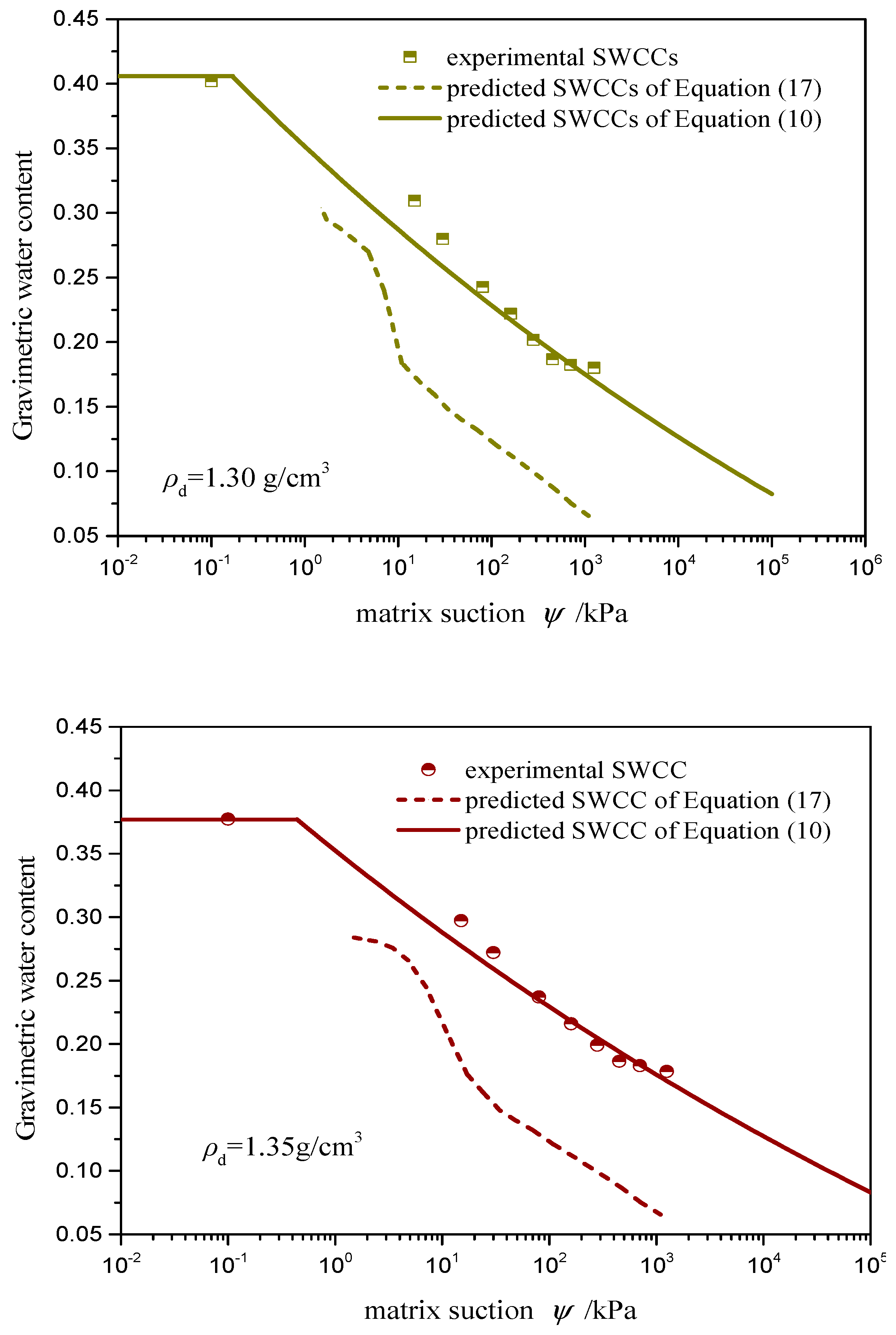
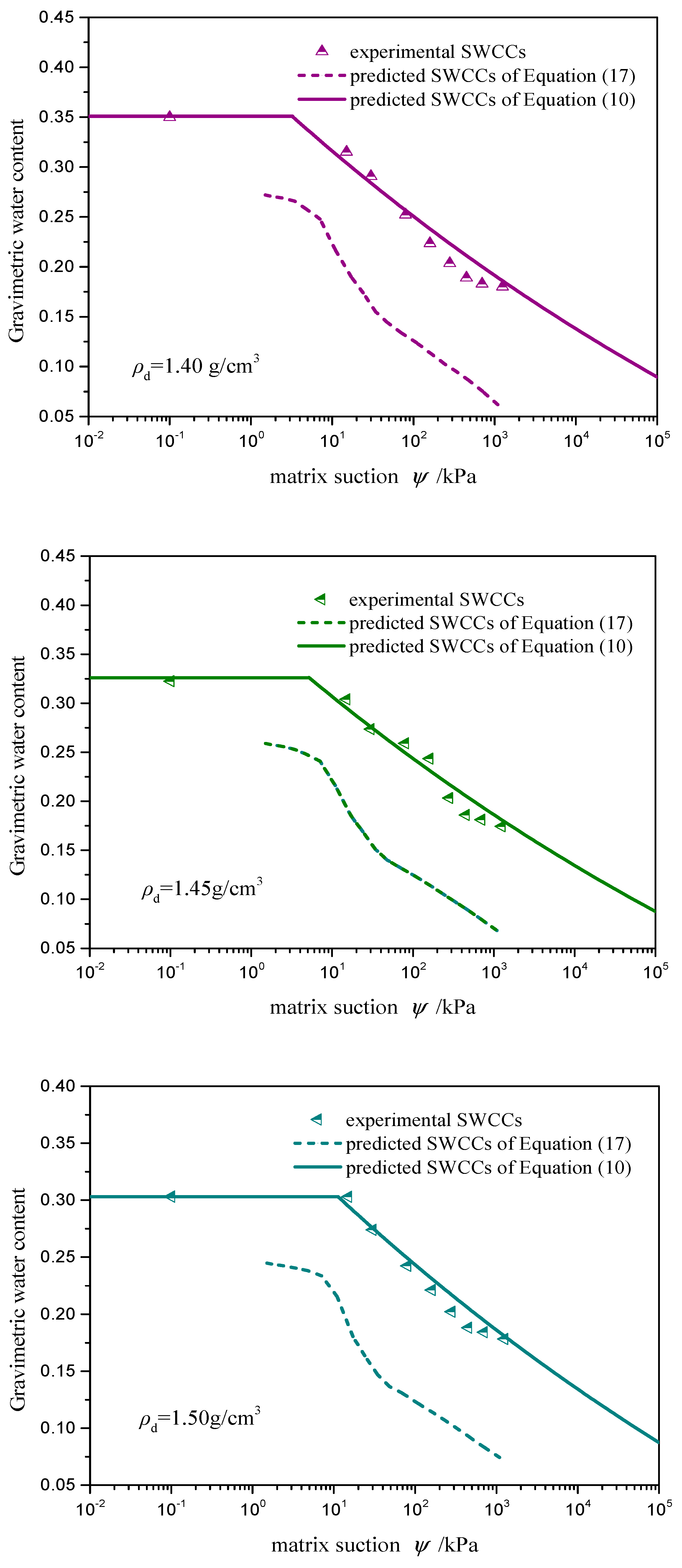
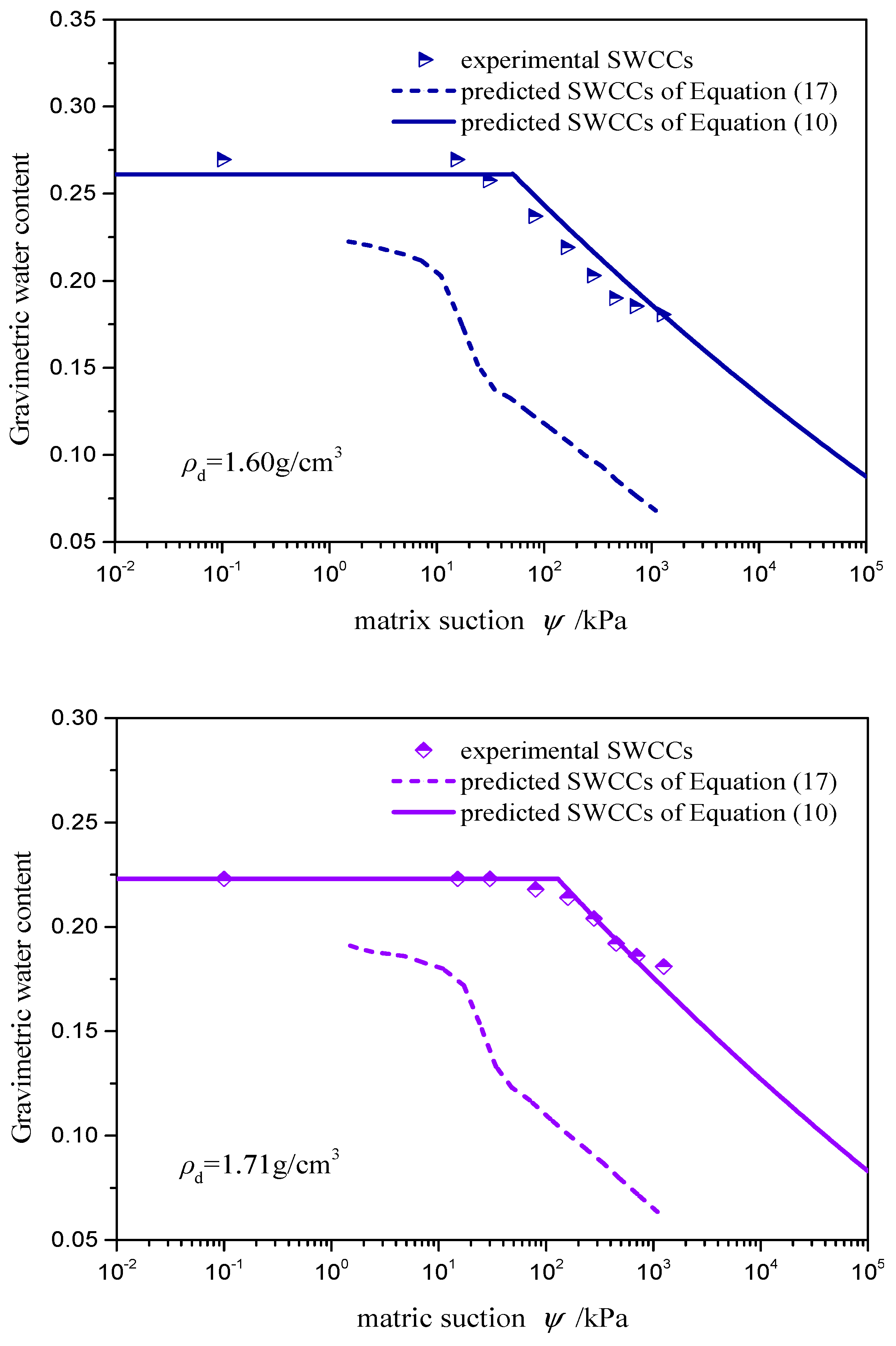
6.3. Validation with SWCC Data

To prove the accuracy of the proposed approach, the prediction results of previous works [28,29,30,31,32,33] are used for comparison. Previous approaches employ Equation (3) to obtain the matrix suction, and Equation (4) to obtain the degree of saturation of water. The specific value of parameters is as follows: α is generally about 0°, θ_m is taken as 130°, T_s is equal to 72.75 uN/m at room temperature, T_m is equal to 483 mN/m at room temperature. To compare with the proposed model, the existing model is converted into the form of gravimetric water content, which is expressed as:

$$\{\begin{array}{l}{\psi }_{}=-\frac{T_s\cos \alpha }{T_m\cos {\theta }_m^{}}p\hfill \\ w={\rho }_{w}V(\le d)\hfill \end{array}$$

(15)

The specific procedure of the proposed model is as follows: the fractal dimension is determined from Equation (12), with the calculation results shown in Table 2. The air-entry value is determined from Equation (14), and the results are shown in Table 3. Combined with Equation (10), the SWCC can then be predicted.

A comparison between the predicted results of Equations (15) and (10) is presented in Figure 7. It is obvious that the predicted SWCCs from Equation (15) is located at the bottom of the experimental SWCCs as a whole, while the predicted SWCCs from Equation (10) are consistent with the experimental SWCCs. The reasons for the large errors of previous work are twofold. One is the difference in contact angle between water and mercury. Another is the difference in PSD and porosity between the MIP sample and SWCC sample, due to the great difference in the sample size of the two test samples. Considering the influence of these factors, a new fractal approach is proposed in this study, where MIP values are used to predict the essential parameters of SWCC (i.e., fractal dimension and air-entry value). As can be seen from Figure 7, the prediction accuracy of proposed approach is higher than that of existing approaches.

The SWCC predicted from proposed model is the horizon when the matrix suction is less than the air-entry value. The proposed model (Equation (10)) takes effect at the stage when Ψ > Ψ_a, while w is approximately assumed to be equal to saturated gravimetric water content at the stage when Ψ ≤ Ψ_a, namely w = e/G_s. Therefore, the slope of the predicted SWCCs has a sudden change at the air-entry value. However, the change of slope in SWCC at the air-entry value is slow in fact, indicating that the fractal approach for predicting SWCCs has a deviation at the air-entry value to some degree.

7. Conclusions

Existing approaches for predicting SWCCs from MIP tests have large deviations, which mainly result from the differences of contact angle, porosity and PSD between the MIP test and SWCC test. Considering these factors, a new prediction approach for SWCC is presented herein, in which the MIP technique is employed to determine the fractal dimension and air-entry value. Because of the effect of sample size on the equivalent connected pore size, a sample scale effect coefficient is introduced into the Young-Laplace equation to greatly enhance the prediction accuracy of the air-entry value. In addition, due to the stronger fractal behaviour and stabler properties of small pores than large pores, it is suggested that only the pore data less than the “critical pore size” be adopted to determine the optimal fractal dimensions. The results of MIP and SWCC tests show that the proposed approach is in good agreement with the measured values.

References

1. Noh, J.H.; Lee, S.R.; Park, H. Prediction of Cryo-SWCC during Freezing Based on Pore-Size Distribution. Int. J. Geomech. 2012, 12, 428–438. [Google Scholar] [CrossRef]
2. Christopher, B. Prediction of soil water retention properties using pore-size distribution and porosity. Can. J. Soil Sci. 2013, 50, 435–450. [Google Scholar]
3. Hu, R.; Chen, Y.F.; Liu, H.H.; Zhou, C.B. A water retention curve and unsaturated hydraulic conductivity model for deformable soils: Consideration of the change in pore-size distribution. Geotechnique 2013, 63, 1389–1405. [Google Scholar] [CrossRef]
4. Arroyo, H.; Rojas, E.; Pérez-Rea, M.D.L.L.; Horta, J. A porous model to simulate the evolution of the soil-water characteristic curve with volumetric strains. C. R. Mécanique 2015, 343, 264–274. [Google Scholar] [CrossRef]
5. Ghanbarian-Alavijeh, B.; Liaghat, A.M. Evaluation of soil texture data for estimating soil water retention curve. Can. J. Soil Sci. 2009, 89, 461–471. [Google Scholar] [CrossRef] [Green Version]
6. Della Vecchia, G.; Dieudonné, A.; Jommi, C.; Charlier, R. Accounting for evolving pore size distribution in water retention models for compacted clays. Int. J. Numer. Anal. Methods Geomech. 2015, 39, 702–723. [Google Scholar] [CrossRef]
7. Mandelbrot, B. The Fractal Geometry of Nature: Updated and Augmented; W. H. Freeman Co.: New York, NY, USA, 1983. [Google Scholar]
8. Perfect, E. Modeling the primary drainage curve of prefractal porous media. Vadose Zone J. 2005, 4, 959–966. [Google Scholar] [CrossRef]
9. Bayat, H.; Neyshaburi, M.R.; Mohammadi, K.; Nariman-Zadeh, N.; Iranneiad, M.; Gregory, A.S. Combination of artificial neural networks and fractal theory to predict soil water retention curve. Comput. Electron. Agric. 2013, 92, 92–103. [Google Scholar] [CrossRef]
10. Tao, G.L.; Wu, X.K.; Xiao, H.L.; Chen, Q.S.; Cai, J.C. A unified fractal model for permeability coefficient of unsaturated soil. Fractals 2019, 27. [Google Scholar] [CrossRef]
11. Li, K.J.; Zeng, F.G.; Cai, J.C.; Sheng, G.L.; Xia, P.; Zhang, K. Fractal characteristics of pores in talyuan formation shale from Hedong goal field, China. Fractals 2018, 26, 1840006. [Google Scholar] [CrossRef]
12. Ghanbarian, B.; Hunt, A.G. Fractals: Concepts and Applications in Geosciences. Available online: https://www.crcpress.com/Fractals-Concepts-and-Applications-in-Geosciences/Ghanbarian-Hunt/p/book/9781498748711 (accessed on 14 November 2017).
13. Tyler, S.W.; Wheatcraft, S.W. Fractal processes in soil water retention. Water Resour. Res. 1990, 26, 1047–1056. [Google Scholar] [CrossRef]
14. Perrier, E.; Rieu, M.; Sposito, G.; Marsily, D.G. Models of the water retention curve for soils with a fractal pore size distribution. Water Resour. Res. 1996, 32, 3025–3031. [Google Scholar] [CrossRef]
15. Xu, Y.F.; Dong, P. Fractal models for the soil-water characteristic of unsaturated soils. Rock Soil Mech. 2002, 23, 400–405. [Google Scholar]
16. Xu, Y.F. Calculation of unsaturated hydraulic conductivity using a fractal model for the pore-size distribution. Comput. Geotech. 2004, 31, 549–557. [Google Scholar] [CrossRef]
17. Perrier, E.; Bird, N.; Rieu, M. Generalizing the fractal model of soil structure: The pore-solid fractal approach. Geoderma 1999, 88, 137–164. [Google Scholar] [CrossRef]
18. Bird, N.; Perrier, E.; Rieu, M. The water retention function for a model of soil structure with pore and solid fractal distributions. Eur. J. Soil Sci. 2000, 51, 55–63. [Google Scholar] [CrossRef]
19. Huang, G.H.; Zhang, R.D. Evaluation of soil water retention curve with the pore-solid fractal model. Geoderma 2005, 127, 52–61. [Google Scholar] [CrossRef]
20. Wang, K.; Zhang, R.D. Estimation of soil water retention curve: An asymmetrical Pore-Solid fractal model. Wuhan Univ. J. Nat. Sci. 2011, 16, 171–178. [Google Scholar] [CrossRef]
21. Ghanbarian-Alavijeh, B.; Millán, H. The relationship between surface fractal dimension and soil water content at permanent wilting point. Geoderma 2009, 151, 224–232. [Google Scholar] [CrossRef]
22. Ghanbarian-Alavijeh, B.; Millán, H.; Huang, G. A review of fractal, prefractal and pore-solid-fractal models for parameterizing the soil water retention curve. Can. J. Soil Sci. 2011, 91, 1–14. [Google Scholar] [CrossRef]
23. Tao, G.L.; Chen, Y.; Yuan, B.; Gan, S.C.; Wu, X.K.; Zhu, X.L. Predicting soil-water retention curve based on NMR technique and fractal theory. J. Geotech. Eng. 2018, 40, 1466–1472. [Google Scholar]
24. Ninjgarav, E.; Chung, S.G.; Jang, W.Y.; Ryu, C.K. Pore size distribution of Pusan clay measured by mercury intrusion porosimetry. KSCE J. Civ. Eng. 2007, 11, 133–139. [Google Scholar] [CrossRef]
25. Lubelli, B.; Winter, D.A.M.; Post, J.A.; van Hees, R.P.J.; Drury, M.R. Cryo-FIB-SEM and MIP study of porosity and pore size distribution of bentonite and kaolin at different moisture contents. Appl. Clay Sci. 2013, 81, 358–365. [Google Scholar] [CrossRef]
26. Wei, X.; Hattab, M.; Fleureau, J.M.; Hu, R. Micro-macro-experimental study of two clayey materials on drying paths. Bull. Eng. Geol. Environ. 2013, 72, 495–508. [Google Scholar] [CrossRef]
27. Zong, Y.T.; Yu, X.L.; Zhu, M.X.; Lu, S. Characterizing soil pore structure using nitrogen adsorption, mercury intrusion porosimetry, and synchrotron-radiation-based X-ray computed microtomography techniques. J. Soils Sediment. 2015, 15, 302–312. [Google Scholar] [CrossRef]
28. Regab, R.; Feyen, J.; Hillel, D. Effect of the method for determining pore size distribution on prediction of the hydraulic conductivity function and of infiltration. Soil Sci. Soc. Am. J. 1982, 134, 141–145. [Google Scholar] [CrossRef]
29. Prapaharan, S.; Altschaeffl, A.G.; Dempsey, B.J. Moisture curve of comp actedclay: Mercury intrusion method. J. Geotech. Eng. 1985, 111, 1139–1142. [Google Scholar] [CrossRef]
30. Kong, L.W.; Tan, L.R. A simple method of determining the soil-water characteristic curve indirectly. In Proceedings of the Asian Conference on Unsaturated Soils, Singapore, 18–19 May 2000. [Google Scholar]
31. Simms, P.H.; Yanful, E.K. Predicting soil-water characteristic curves of compacted plastic soils from measured pore size distributions. Géotechnique 2002, 52, 269–278. [Google Scholar] [CrossRef]
32. Zhang, L.M.; Li, X. MicroPorosity Structure of Coarse Granular Soils. J. Geotech. Geoenviron. Eng. 2010, 136, 1425–1436. [Google Scholar] [CrossRef]
33. Zhang, Z.L.; Cui, Z.D. Effects of freezing-thawing and cyclic loading on pore size distribution of silty clay by mercury intrusion porosimetry. Cold Reg. Sci. Technol. 2018, 145, 185–196. [Google Scholar] [CrossRef]
34. Zhang, J.R.; Tao, G.L.; Huang, L.; Yuan, L. Porosity models for determining the pore-size distribution of rocks and soils and their applications. Chin. Sci. Bull. 2010, 55, 3960–3970. [Google Scholar] [CrossRef]
35. Tao, G.L.; Zhang, J.R. Two categories of fractal models of rock and soil expressing volume and size- distribution of pores and grains. Chin. Sci. Bull. 2009, 54, 4458–4467. [Google Scholar] [CrossRef]
36. Tan, L.R.; Kong, L.W. Special Geotechnical Soil Science, 1st ed.; Science Press: Beijing, China, 2006. [Google Scholar]
37. Zhao, M.H. Soil Mechanics and Foundation Engineering, 3rd ed.; Wuhan University Technology Press: Wuhan, China, 2009. [Google Scholar]
38. Tao, G.L.; Zhu, X.L.; Hu, Q.Z.; Zhuang, X.S.; He, J.; Chen, Y. Critical pore-size phenomenon and intrinsic fractal characteristic of clay in the process of compression. Rock Soil Mech. 2019, 40, 81–90. [Google Scholar]
39. Ghanbarian, B.; Hunt, A.G. Improving unsaturated hydraulic conductivity estimation in soils via percolation theory. Geoderma 2017, 303, 9–18. [Google Scholar] [CrossRef]
Figure 1. Schematic diagram of an air-water interface and a mercury-air interface. (a) air-water interface; (b) mercury-air interface.
Energies 12 00752 g001
Figure 2. The influence of parameters on SWCC: (a) fractal dimension, (b) air-entry value.
Energies 12 00752 g002
Figure 3. Diagram of the sample scale effect for the equivalent connected pore size. (a) ichnography for two layers; (b) ichnography for three layers; (c) cross section for two layers and (d) cross section for three layers.
Energies 12 00752 g003aEnergies 12 00752 g003b
Figure 4. The experimental data of MIP tests.
Energies 12 00752 g004
Figure 5. The cumulative pore volume curves of different dry densities.
Energies 12 00752 g005
Figure 6. Determination of fractal dimension D. (a) neglecting “critical pore size”; (b) considering “critical pore size”.
Energies 12 00752 g006
Figure 7. Comparison between experimental results and predicted SWCCs from Equation (15) and Equation (10).
Energies 12 00752 g007aEnergies 12 00752 g007bEnergies 12 00752 g007c