Analyzing Oil Price Shocks and Exchange Rates Movements in Korea using Markov Regime-Switching Models

Abstract

Korea imports all of its crude oil, and is the world’s fifth largest oil importing country. We analyze the effects of oil prices, interest rates, consumer price indexes $(CPI$s), and industrial production indexes ($IPI$s) on the regime shift behavior of the Korean exchange rates against the USA from January 1991 to March 2019. We use the Markov regime switching model (MRSM) to detect the regime shift behavior of the movements of Korean exchange rates. In order to select the optimal MRSM, we fit a total of 30 models considering four explanatory variables. The selected model based on Akaike information criteria $\left(AIC\right)$ and maximum log likelihood $\left(MLL\right)$ includes the log-differentials of oil prices, the log-differentials of $CPI$s compared to those of the US, and its own auto-regressive terms. Based on the selected MRSM model, throughout all markets, we find evidence to support the existence of two distinct regimes: a stable regime with low-volatility, and an unstable regime with high-volatility. The regime with high-volatility includes the Asian financial crisis of 1997 and the global financial crisis of 2008–2009 in the Korean exchange rates market. In the regime with low-volatility, the Korean exchange rates are not significantly influenced by any of the explanatory variables, except for its own auto-regressive terms. In the regime with high-volatility, the Korean exchange rates are significantly influenced by the $CPI$s and oil prices. The transition probability from the regime with low-volatility to the regime with high-volatility is about ten times that of the opposite case.

1. Introduction

Oil prices have fluctuated over the last 30 years. Oil prices per barrel have risen to over $140 and dropped to below $20. Although energy dependence on oil has declined in the past, oil is still one of the most important sources of energy. Thus, rising oil prices have a huge impact on the economies of countries, which is especially true in those countries that mostly export or import oil. The greater the energy dependence on oil, the greater the impact oil has on the economy. In particular, Korea imports all of its oil and is the one of the world’s top 10 oil importers. As a result, oil price fluctuations have a large impact on the trade balance and also on the supply and demand of dollars in the foreign exchange market. This seems to have further led to fluctuations in exchange rates. Thus, analyzing how oil prices affect the exchange rates has been one of the major concerns of economists. Previous studies which have analyzed the relationship between oil prices and exchange rates are Amano and Van Norden [1], Amano and Van Norden [2], Chaudhuri and Daniel [3], Chen and Chen [4], Lizardo and Mollick [5], Basher et al. [6], Aloui et al. [7], Chen et al. [8], Volkov and Yuhn [9], Chen et al. [10], Basher et al. [11], Yang et al. [12], and so on (see

Table 1. Previous studies on the dynamics of oil prices and exchange rates.

Authors	Countries	Periods	Methods	Main Results
Amano and Van Norden [1]	Germany, Japan, USA	1973.01–1993.06	Cointegration, granger causality, FMOLS	Oil shocks could be the most important factor determining real exchange rates in the long run
Amano and Van Norden [2]	USA	1972.02–1993.01	ECM (error correction model), Granger causality	Oil prices may have been the dominant source of persistent real shocks
Chaudhuri and Daniel [3]	16 OECD countries	1973.01–1996.02	ECM (error correction model), Granger causality	US dollar real exchange rates are due to the non-stationarity in the real price of oil.
Chen and Chen [4]	G7 countries	1972.01–2005.10	Panel cointegration, FMOLS, DOLS, and PMG	The real oil prices may have been the dominant source of real exchange rate movements
Lizardo and Mollick [5]	USA	1970s–2008	VECM	Oil price is significant in the movements of the exchange rate
Basher et al. [6]	Emerging economics	1988.01–2008.12	Structural VAR	A positive oil price shock leads to an immediate drop in the exchange rate
Aloui et al. [7]	European union, Canada, UK, Swiss, Japan	2000–2011	copula-GARCH	Evidence of significant and symmetric dependence for almost all the oil-exchange rate pairs. Increases in crude oil prices were found to coincide with a depreciation of the dollar
Chen et al. [8]	USA	1992.08–2011.12 (weekly)	GARCH, CARR, CARR-MIDAS	Crude oil returns are more negatively associated with US dollar returns when the US dollar depreciates, as compared to when it appreciates
Volkov and Yuhn [9]	Russia, Brazil, Mexico, Canada, Norway	1998.02–2012.08	GARCH-M, VECM	Oil price is significant on exchange rates in Russia, Brazil, and Mexico
Chen et al. [10]	16 OECD countries	1990.01–2014.12	Structural VAR	Oil price shocks can explain about 10–20% of long-term variations in exchange rates
Basher et al. [11]	9 countries 1	Varies by each country 2	Markov switching model	The significant exchange rate appreciation pressures in oil exporting economies after oil demand shock
Yang et al. [12]	10 countries 3	1999.01–2014.12	A wavelet coherence analysis	The degree of co-movement between the crude oil price and the exchange rates deviates over time

¹ Analysis is conducted for a group of oil exporting countries (Brazil, Canada, Mexico, Norway, Russia, and the United Kingdom) and oil importing countries (India, Japan, South Korea). ² For Canada, Norway, India, Japan, and the United Kingdom, models are estimated over the period February 1976 to February 2014. For the other countries the estimation period is: Brazil (February 1995 to February 2014), Mexico (December 1993 to February 2014), Russia (February 1998 to February 2014), and South Korea (May 1981 to February 2014). ³ Brazil, Canada, Mexico, and Russia are treated as oil-exporting countries, and the EU, India, Japan, and South Korea are treated as oil-importing countries.

).

Most of these studies not only analyzed the direct relationship between oil prices and the exchange rates, but also analyzed the relationships with other macroeconomic variables, using the macroeconomic model. Most of the analyses focused on developed countries, including the US, and oil-exporting countries, such as Brazil, Canada, Mexico, Norway, Russia, and the United Kingdom. Basher et al. [11] and Yang et al. [12] included Korea in their analyses; however, there have been no studies that have analyzed only Korea in-depth.

The methodologies used by most of the studies vary from the error correction model (ECM), the vector error correction model (VECM), structural vector auto-regression (SVAR), generalized auto-regressive conditional heteroscedasticity (GARCH), and generalized auto-regressive conditional heteroscedasticity M (GARCH-M). Recently, methodologies such as the Markov regime switching model (Basher et al., [11]) and wavelet coherence analyses (Yang et al., [12]) have been introduced. The methodologies introduced so far are presented in Table 1.

This study analyzes how oil prices affect the Korean exchange rates in both stable and unstable regimes using the Markov regime switching model (MRSM), taking into account other factors such as interest rates, economic growth, and price level. This study differs from previous studies in several aspects. First, most studies on the relationship between oil prices and exchange rates except Basher et al. [11] have used econometric methodologies such as ECM, VECM, SVAR, GARCH, and GARCH-M. Often a pooled series consists of a few subgroups or regimes with different variances corresponding to different economic situations. The impact of oil prices on the exchange rates is expected to vary depending on regimes. Therefore, this study looks for underlying regimes using the Markov regime switching model (MSRM), fits a separate model in each regime, and then examines the effect of oil prices along with major macroeconomic explanatory variables on the exchange rates. Since the regimes are expected to explain many errors, the model in each regime tends to be simple.

Second, not only oil prices but also macroeconomic factors such as price levels, income, and interest rates are the major factors that influence the exchange rates. Except for Volkov and Yuhn [9] and Basher et al. [11], most studies have analyzed only the direct relationship between oil prices and exchange rates. This study analyzes the effects of oil prices on exchange rates in each regime under the correlation with these macro-economic variables. In addition to discovering regimes, this MRSM analysis tests the significance of oil prices and various macroeconomic variables in each regime. Since regimes stand for different economic situations, the significance of variables also changes depending on regimes.

Third, this study is limited to Korea. Crude oil is entirely imported in Korea and Korea was one of the world’s top 10 oil importers. The 10 countries that imported the highest dollar value worth of crude oil during 2018 are 1. China: US$239.2 billion (20.2% of total crude oil imports), 2. United States: $163.1 billion (13.8%), 3. India: $114.5 billion (9.7%), 4. Japan: $80.6 billion (6.8%), 5. South Korea: $80.4 billion (6.8%), 6. Netherlands: $48.8 billion (4.1%), 7. Germany: $45.1 billion (3.8%), 8. Spain: $34.2 billion (2.9%), 9. Italy: $32.6 billion (2.8%) and 10. France: $28.5 billion (2.4%) (http://www.worldstopexports.com/crude-oil-imports-by-country/). In 2018, Korea was the world’s fifth largest oil importer. According to Korean Customs Service statistics, crude oil imports in 2018 were worth 80,393 million dollars. This amount of imported crude oil accounted for 15% of Korea’s total imports in 2018. Reflecting this economic situation in Korea, this analysis provides unique results for Korea.

Fourth, this study analyzes the effects of movement of explanatory variables on the movement of exchange rates, while most of previous studies have analyzed the direct relationship between exchange rates and explanatory macroeconomic variables. Throughout this paper, we use the US data as the basis for comparison.

Therefore, we use the MRSMs, developed by Hamilton [13]. This methodology is further developed into Markov switching auto-regressive conditional heteroscedasticity (MS-ARCH, Cai [14]), Markov switching generalized auto-regressive conditional heteroscedasticity (MS-GARCH, Gray [15]), and Markov switching exponential generalized auto-regressive conditional heteroscedasticity (MS-EGARCH, Henry [16]), among others. The MSRM used in this study was also used in Kim et al. [17] and Kim et al. [18].

We examine the regime shift behavior of exchange rates associated with oil prices, interest rates, consumer price indices, and industrial production indices in the Korean foreign exchange market. For this, we apply the two-regime MRSM (Hamilton, [13]) using monthly data from January 1991 to March 2019.

The remainder of this paper is organized as follows. In Section 2, the data and the MSRM are explained in detail. In Section 3, the model selection is performed and empirical estimation results are presented based on the selected MRSM, and Section 4 discusses the statistical validity of our model and assumptions. Finally, the conclusions drawn from this study are presented in Section 5.

2. Data and Methods

All monthly data, except for the oil prices, used in this paper are from the OECD (Organization for Economic Cooperation and development) data set (OECD.stat) from January 1991 to March 2019. The monthly Korean exchange rates are expressed as the won value needed to purchase one US dollar. The monthly short-run interest rates measured in % are from the monthly monetary and financial statistics data set of the OECD. The monthly consumer price indices (with the index of 2015 being 100) are from the consumer price indices ($CPI$s) complete database of the OECD, and the monthly industrial production indices (with the index of 2015 being 100) are from the production and sales data set of the OECD. The monthly oil prices which are the CIF (Cost Insurance and Freight) oil importing prices of Asia measured in US dollars are from KESIS (Korea Energy Statistics Information System) of the Korea Energy Economics Institute.

The primary purpose of this study is to analyze how the movement of oil prices affects the movement of the Korean exchange rates in each regime in terms of regime shift behavior. Our research is based on the monetary model of exchange rates determination which has lead emergence of the dominant exchange rates model in early 1970s and henceforward remained as an important exchange rate paradigm (Frenkel [19], Mussa [20,21,22], Bilson [23]). Following the monetary model, the exchange rates are determined by the relative supply and demand of money between two given countries. The money demand is determined by price level, income, interest rates, and other factors including oil prices. Meese and Rogoff [24,25] conducted the seminal work using monetary models to forecast exchange rates. They regressed the log of exchange rates on various combinations of relative macroeconomic variables which were typically included in the monetary model of exchange rates determination.

Recently, Volkov and Yuhn [9] identified some relevant factors that affect the exchange rates between the United States and the corresponding countries on the basis of the monetary model of exchange rates determination. The fundamental factors include interest rates differentials, income (or production) differentials, and inflation rates differentials between two countries. They excluded the money supply variable from the exchange rates determination model to avoid any possible multicollinearity between the money supply and the determining variables of the exchange rates. Since they use monthly data for the analysis of exchange rates movements, and since monthly GDP figures are not available, industrial production is used as a proxy for income.

We consider some relevant variables that affect the exchange rates between Korea and the USA as in Volkov and Yuhn [9]. Oil prices are added to the fundamental factors including interest rates differentials, production differentials, and inflation rates differentials between the two countries. Here, industrial production index $\left(IPI\right)$ and consumer price index $\left(CPI\right)$ are set as indices representing production and inflation, respectively.

The two-regime Markov switching model by Hamilton [1] is an adequate approach to analyze the impact of these factors (oil prices, interest rates differentials, $CPI$s differentials, and $IPI$s differentials) on the movements of Korean exchange rates. In terms of methodology, the auto-regressive terms are considered as in the Hamilton models [1]. The MRSM following Hamilton [1] assumes that there are two regimes with different volatilities, and that the processes switch between the two regimes according to the transition probabilities of the Markov process. Regime 1 consists of low-volatility periods and regime 2 consists of high-volatility periods. Regime 2 is used to identify unstable economic situations.

In this paper, we assume that the logarithms of exchange rates follow a normal distribution as the logarithms of return rates in equity markets follow a Brownian motion (Osborne, [26]). Often in economic data, the log-transformation reinforces the normality assumption and using differentials reinforces stationarity of the process. At time $t$, let $L{E}_t$ be the logarithm of the monthly changes in exchange rates compared to the ones from the previous month as follows (Ayodeji [27]):

$$L{E}_t=\log \left(\frac{Exchange Rat{e}_t}{Exchange Rat{e}_{t-1}}\right),$$

(1)

$L{E}_t$ lies in one of the two regimes $S_t$, where $S_t$ is 1 or 2. $L{E}_t$ is $\Delta \log \left(Exchange Rat{e}_t\right)$ in the interval $\left[t-1, t\right)$, which is the change of $\log \left(Exchange Rat{e}_t\right)$. If we consider the time change as $\Delta t=t-\left(t-1\right)=1,$ then $L{E}_t$ is the change rate in $\left[t-1, t\right)$. Assuming that the series is an infinite continuous process, $L{E}_t$ is an approximate derivative of $\log (Exchange Rat{e}_t)$ at $\left(t-1\right)$. That is, $L{E}_t$ is the slope of the tangent line to $\log (Exchange Rat{e}_t)$ which means instantaneous change rate of $\log (Exchange Rat{e}_t)$ at $\left(t-1\right)$. Now let us call $L{E}_t$ log-differential of exchange rates. Since regime shift behaviors of $(Exchange Rat{e}_t)$ and $L{E}_t$ should match, we investigate regimes of exchange rates using $L{E}_t$. Note that $L{E}_t$ stands for changes of exchange rates.

Similarly, we transform the four explanatory variables. First, $RIN{T}_{\mathrm{t}}, RCP{I}_{\mathrm{t}},$ and $RIP{I}_{\mathrm{t}}$ are the ratios of short-run interest rates, the ratio of consumer price indices and ratio of industrial production indices between Korea and the USA, respectively. Then, the log-differentials of these ratios of macroeconomic variables are obtained as $LOI{L}_t$, $LRIN{T}_t, LRCP{I}_t$, and $LRIP{I}_t$. The relative differences of these fundamental variables between the two countries are expected to affect US exchange rates in Korea, as confirmed by Volkov and Yuhn [9]. However, this study regards the variable ratio between the two countries, instead of their direct differences like the study of Volkov and Yuhn [9], because the Korean exchange rates are expressed as ratios with the US dollars as its denominator. The similar form of log-differentials of variables provides the same intrinsic explanation as before.

$$LOI{L}_t=\log \left(\frac{Oil Pric{e}_t}{Oil Pric{e}_{t-1}}\right),$$

(2)

$$LRIN{T}_t=\log \left(\frac{RIN{T}_t}{RIN{T}_{t-1}}\right), \mathrm{where} RIN{T}_{\mathrm{t}}= \frac{Interest rate of Korea at t}{Interest rate of USA at t},$$

(3)

$$LRCP{I}_t=\log \left(\frac{RCP{I}_t}{RCP{I}_{t-1}}\right), \mathrm{where} RCP{I}_{\mathrm{t}}= \frac{Consumer price index of Korea at t}{Consumer price index of USA at t},$$

(4)

$$LRIP{I}_t=\log \left(\frac{RIP{I}_t}{RIP{I}_{t-1}}\right),\mathrm{where} RIP{I}_{\mathrm{t}}= \frac{Industrial production index of Korea at t}{Industrial production index of USA at t},$$

(5)

Note that there are two ratios in Equations (3)–(5). First, the ratio between Korea and the USA is evaluated. Secondly, the ratio between time $t$ and time $\left(t-1\right)$ is evaluated. Finally, log-transformation is applied. The $LR$ in front of the variable name stands for log-transformation of the ratio of the ratio. Therefore, we indirectly observe changes in movements of exchange rates through its log-differentials. In each regime, the standard deviation is that of the log-differentials of exchange rates.

The MRSM with the four explanatory variables we consider can be written as follows:

$$L{E}_t\left|s_t={\beta }_{0s_t}+{\beta }_{1s_t}L{E}_{t-1}+{\beta }_{2s_t}LOI{L}_t+{\beta }_{3s_t}LRIN{T}_t+{\beta }_{4s_t}LRCP{I}_t+{\beta }_{5s_t}LRIP{I}_t +{\epsilon }_t\right|s_t,$$

(6)

where ${\epsilon }_t|s_t~N\left(0,{\sigma }_{s_t}^2\right).$ Our model assumes that the exchange rates switch between the two regimes based on the Markov transition probabilities which are denoted by

$$p_{ij}=Pr\left[s_{t+1}=j|s_t=i\right], i=1, 2, j=1, 2,$$

(7)

where, $p_{ij}$ is the transition probability from state $i$ to state $j$, $p_{i1}+p_{i2}=1$, for $i$ = 1, 2. The oil prices, the interest rates, the $CPI$s and the $IPI$s do not switch. We assume that ${\sigma }_1^2<{\sigma }_2^2$. The parameter space $\mathsf{\Theta }$ is as follows

$$\mathsf{\Theta }=\left\{{\beta }_{0s_t}, {\beta }_{1s_t},{\beta }_{2s_t}, {\beta }_{3s_t},{\beta }_{4s_t},{\beta }_{5s_t} {\sigma }_{s_t}^2, p_{12, }, p_{21}\right\}, s_t=1 \mathrm{or} 2.$$

(8)

The filtered probabilities of $s_t$ are defined as $P(s_t=i |Z_t; \Theta )$ for $i=1,2$, where $Z_t$ stands for all observations up to time $\mathrm{t}$. In our empirical studies, the process at time $\mathrm{t}$ is said to be in regime 1 (with low-volatility) if its estimated filtered probability of regime 1 is greater than that of regime 2. Otherwise, the process at time $\mathrm{t}$ is said to be in regime 2 (Sanchez-Espigares and Jose [28], Kuan [29]).

For model selection, we first fit the full model. Secondly, based on stepwise selection method, we select the most appropriate model using Akaike information criterion ($AIC$) criterion. Third, the Wilks test is performed based on the maximum log-likelihood ($MLL$) to select the final model based on Maximum Likelihood Estimator ($MLE$). If the sample size is large, the $\left(-2MLL\right)$ difference between the general model and restricted model is asymptotically a chi-squared distribution, with the degrees of freedom as the dimension difference of the two parameter spaces when the restricted model is correct.

The restricted model is assumed under the null hypothesis and the general model is used under the alternative hypothesis. If $ML{L}_r$ and $ML{L}_g$ are the $MLL$ of the restricted model and the $MLL$ of the more general model, respectively, and $d_i$ is the number of parameters to be estimated in model $i$, then the difference in $MLL$ asymptotically follows a chi-squared distribution for a large sample:

$$\Delta \left(-2MLL\right)=\left(-2ML{L}_r\right)-\left(-2ML{L}_g\right)\to {\chi }^2\left(d_g-d_r\right),$$

(9)

If the difference in $MLL$ between any two selected models is significant, then the general model is selected. In addition to the $MLL$, we use the $AIC$ which considers a penalty to increment of dimension of the model.

$$AIC= -2MLL+2n_{par}$$

(10)

where $n_{par}$ is the number of parameters to be estimated in the model. “The model with smaller $AIC$ is better.” (Akaike [30]; Akaike [31]; Pinheiro and Bates, [32]; Rice [33]). The $AIC$ is now one of the most popular model selection criteria in machine learning. Starting from the full model in Equation (6), the variables will be first selected based on $AIC$, and then significance of each variable in the selected model is tested based on $\Delta \left(-2MLL\right)$ in Equation (9). We use the msmFit function (Sanchez-Espigares and Jose, [28]) and the stepAIC function (Venables and Ripley, [34]) in R 3.3.1. Throughout the paper, $p$-values less than 0.10 are considered to be statistically significant.

3. Results

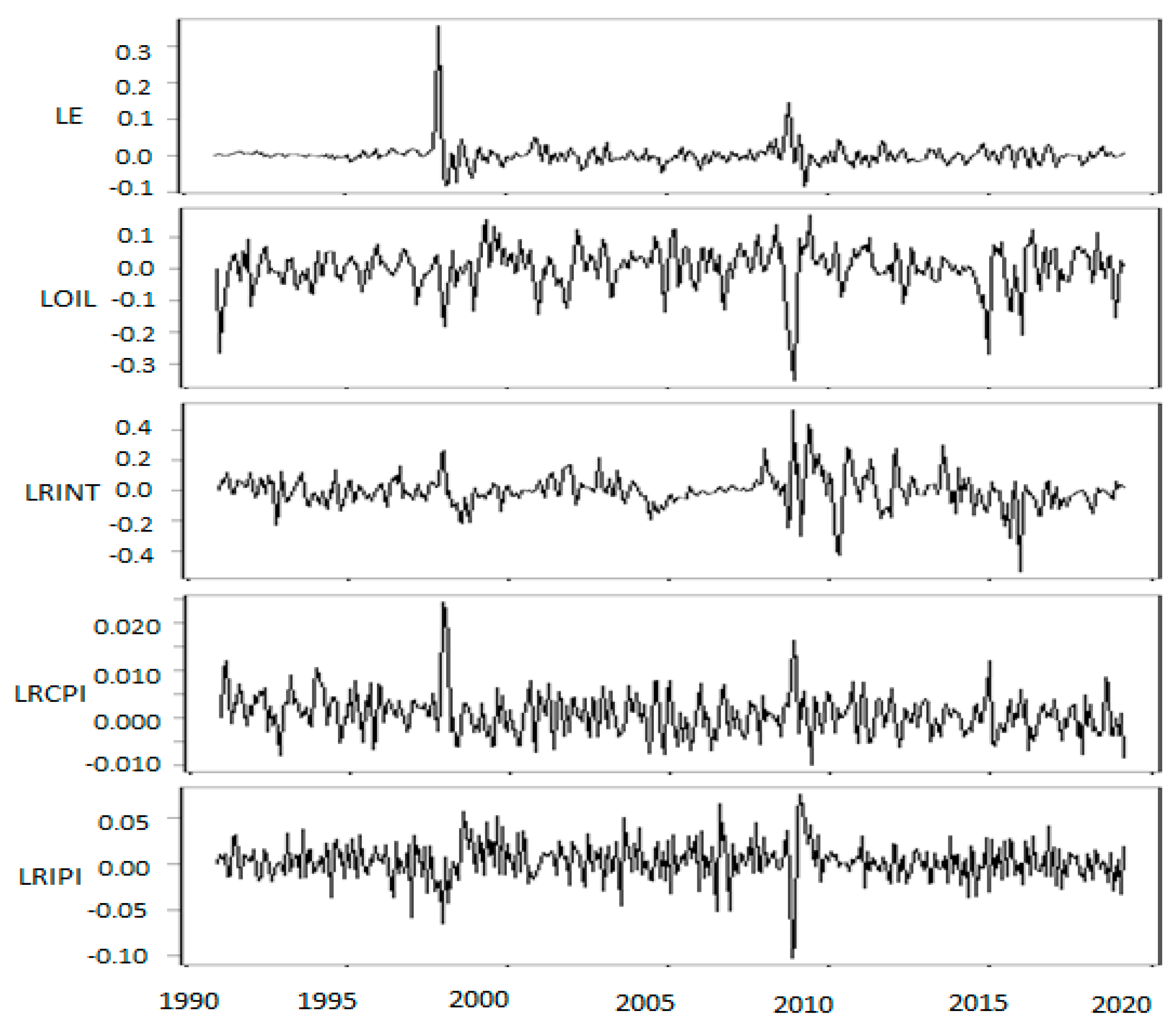
The plots of Figure 1 show time series from January 1991 to March 2019 in the Korean exchange rates market: (1) $LE$ (exchange rates), (2) $LOIL$ (oil prices) (3) $LRINT$ (interest rates between Korea and the USA.), (4) $LRCPI$ ($CPI$s between Korea and USA), and (5) $LRIPI$ ($IPI$s between Korea and the USA.). Co-movements of high peaks and low valleys are observed in these processes during the Asian financial crisis of 1997 and the global financial crisis of 2008–2009.

With exchange rates as the response variable, we fit the following thirty two-regime switching models, as shown in

Table A1. The Markov Regime Switching Models for exchange rates along with oil prices, interest rates, CPI’s and IPI’s.

Model Number	Equation
1(1)	$L{E}_t\left|s_t={\beta }_{0s_t}+{\beta }_{2s_t}LOI{L}_t+{\epsilon }_t\right|s_t$
1(1p)	$L{E}_t\left|s_t={\beta }_{0s_t}+{\beta }_{1s_t}L{E}_{t-1}+{\beta }_{2s_t}LOI{L}_t+{\epsilon }_t\right|s_t$
1(2)	$L{E}_t\left|s_t={\beta }_{0s_t}+{\beta }_{3s_t}LRIN{T}_t+{\epsilon }_t\right|s_t$
1(2p)	$L{E}_t\left|s_t={\beta }_{0s_t}+{\beta }_{1s_t}L{E}_{t-1}+{\beta }_{3s_t}LRIN{T}_t+{\epsilon }_t\right|s_t$
1(3)	$L{E}_t\left|s_t={\beta }_{0s_t}+{\beta }_{4s_t}LRCP{I}_t +{\epsilon }_t\right|s_t$
1(3p)	$L{E}_t\left|s_t={\beta }_{0s_t}+{\beta }_{1s_t}L{E}_{t-1}+{\beta }_{4s_t}LRCP{I}_t+{\epsilon }_t\right|s_t$
1(4)	$L{E}_t\left|s_t={\beta }_{0s_t}+{\beta }_{5s_t}LRIP{I}_t +{\epsilon }_t\right|s_t$
1(4p)	$L{E}_t\left|s_t={\beta }_{0s_t}+{\beta }_{1s_t}L{E}_{t-1}+{\beta }_{5s_t}LRIP{I}_t +{\epsilon }_t\right|s_t$
2(1)	$L{E}_t\left|s_t={\beta }_{0s_t}+{\beta }_{2s_t}LOI{L}_t+{\beta }_{3s_t}LRIN{T}_t+{\epsilon }_t\right|s_t$
2(1p)	$L{E}_t\left|s_t={\beta }_{0s_t}+{\beta }_{1s_t}L{E}_{t-1}+{\beta }_{2s_t}LOI{L}_t+{\beta }_{3s_t}LRIN{T}_t+{\epsilon }_t\right|s_t$
2(2)	$L{E}_t\left|s_t={\beta }_{0s_t}+{\beta }_{2s_t}LOI{L}_t+{\beta }_{4s_t}LRCP{I}_t+{\epsilon }_t\right|s_t$
2(2p)	$L{E}_t\left|s_t={\beta }_{0s_t}+{\beta }_{1s_t}L{E}_{t-1}+{\beta }_{2s_t}LOI{L}_t+{\beta }_{4s_t}LRCP{I}_t+{\epsilon }_t\right|s_t$
2(3)	$L{E}_t\left|s_t={\beta }_{0s_t}+{\beta }_{2s_t}LOI{L}_t+{\beta }_{5s_t}LRIP{I}_t +{\epsilon }_t\right|s_t$
2(3p)	$L{E}_t\left|s_t={\beta }_{0s_t}+{\beta }_{1s_t}L{E}_{t-1}+{\beta }_{2s_t}LOI{L}_t+{\beta }_{5s_t}LRIP{I}_t +{\epsilon }_t\right|s_t$
2(4)	$L{E}_t\left|s_t={\beta }_{0s_t}+{\beta }_{3s_t}LRIN{T}_t+{\beta }_{4s_t}LRCP{I}_t+{\epsilon }_t\right|s_t$
2(4p)	$L{E}_t\left|s_t={\beta }_{0s_t}+{\beta }_{1s_t}L{E}_{t-1}+{\beta }_{3s_t}LRIN{T}_t+{\beta }_{4s_t}LRCP{I}_t+{\epsilon }_t\right|s_t$
2(5)	$L{E}_t\left|s_t={\beta }_{0s_t}+{\beta }_{3s_t}LRIN{T}_t+{\beta }_{5s_t}LRIP{I}_t +{\epsilon }_t\right|s_t$
2(5p)	$L{E}_t\left|s_t={\beta }_{0s_t}+{\beta }_{1s_t}L{E}_{t-1}+{\beta }_{3s_t}LRIN{T}_t+{\beta }_{5s_t}LRIP{I}_t +{\epsilon }_t\right|s_t$
2(6)	$L{E}_t\left|s_t={\beta }_{0s_t}+{\beta }_{4s_t}LRCP{I}_t+{\beta }_{5s_t}LRIP{I}_t +{\epsilon }_t\right|s_t$
2(6p)	$L{E}_t\left|s_t={\beta }_{0s_t}+{\beta }_{1s_t}L{E}_{t-1}+{\beta }_{4s_t}LRCP{I}_t+{\beta }_{5s_t}LRIP{I}_t +{\epsilon }_t\right|s_t$
3(1)	$L{E}_t\left|s_t={\beta }_{0s_t}+{\beta }_{2s_t}LOI{L}_t+{\beta }_{3s_t}LRIN{T}_t+{\beta }_{4s_t}LRCP{I}_t+{\epsilon }_t\right|s_t$
3(1p)	$L{E}_t\left|s_t={\beta }_{0s_t}+{\beta }_{1s_t}L{E}_{t-1}+{\beta }_{2s_t}LOI{L}_t+{\beta }_{3s_t}LRIN{T}_t+{\beta }_{4s_t}LRCP{I}_t+{\epsilon }_t\right|s_t$
3(2)	$L{E}_t\left|s_t={\beta }_{0s_t}+{\beta }_{2s_t}LOI{L}_t+{\beta }_{3s_t}LRIN{T}_t+{\beta }_{5s_t}LRIP{I}_t +{\epsilon }_t\right|s_t$
3(2p)	$L{E}_t\left|s_t={\beta }_{0s_t}+{\beta }_{1s_t}L{E}_{t-1}+{\beta }_{2s_t}LOI{L}_t+{\beta }_{3s_t}LRIN{T}_t+{\beta }_{5s_t}LRIP{I}_t +{\epsilon }_t\right|s_t$
3(3)	$L{E}_t\left|s_t={\beta }_{0s_t}+{\beta }_{2s_t}LOI{L}_t+{\beta }_{4s_t}LRCP{I}_t+{\beta }_{5s_t}LRIP{I}_t +{\epsilon }_t\right|s_t$
3(3p)	$L{E}_t\left|s_t={\beta }_{0s_t}e+{\beta }_{1s_t}L{E}_{t-1}+{\beta }_{2s_t}LOI{L}_t+{\beta }_{4s_t}LRCP{I}_t+{\beta }_{5s_t}LRIP{I}_t +{\epsilon }_t\right|s_t$
3(4)	$L{E}_t\left|s_t={\beta }_{0s_t}+{\beta }_{3s_t}LRIN{T}_t+{\beta }_{4s_t}LRCP{I}_t+{\beta }_{5s_t}LRIP{I}_t +{\epsilon }_t\right|s_t$
3(4p)	$L{E}_t\left|s_t={\beta }_{0s_t}+{\beta }_{1s_t}L{E}_{t-1}+{\beta }_{3s_t}LRIN{T}_t+{\beta }_{4s_t}LRCP{I}_t+{\beta }_{5s_t}LRIP{I}_t +{\epsilon }_t\right|s_t$
4(1)	$L{E}_t\left|s_t={\beta }_{0s_t}+{\beta }_{2s_t}LOI{L}_t+{\beta }_{3s_t}LRIN{T}_t+{\beta }_{4s_t}LRCP{I}_t+{\beta }_{5s_t}LRIP{I}_t +{\epsilon }_t\right|s_t$
4(1p)	$L{E}_t\left|s_t={\beta }_{0s_t}+{\beta }_{1s_t}L{E}_{t-1}+{\beta }_{2s_t}LOI{L}_t+{\beta }_{3s_t}LRIN{T}_t+{\beta }_{4s_t}LRCP{I}_t+{\beta }_{5s_t}LRIP{I}_t +{\epsilon }_t\right|s_t$

in Appendix A: (1) eight models with one explanatory variable (from 1 (1) to 1 (4p)); (2) twelve models with two explanatory variables (from 2 (1) to 2 (6p)); (3) eight models with three explanatory variables (from 3 (1) to 3 (4p)); and (4) two models with all four explanatory variables (from 4 (1) and 4 (1p)). For each model, p stands for the model with the auto-regressive terms of the exchange rates.

We consider the two model selection criteria: $MLL$ and $AIC$. We first fit the full model in Equation (6). Then, the model with smallest $AIC$ is selected based on the stepwise selection method. In order to reach the final model, significance of each variable in the selected model is further tested one-by-one based on $\Delta \left(-2MLL\right)$ in Equation (9) and the backward selection method. Note that the degrees of freedom is 2 since we test one variable at a time which corresponds to the two coefficients, one for the low-volatility period and the other for the high-volatility period. At the significance level 0.1, if $\Delta \left(-2MLL\right)>{\chi }_{0.10}^2\left(2\right)=4.61$, the variable is said to be significant and remain in the model. Otherwise, it is removed.

For the use of MLL in model selection for MRSM, Hardy [17] mentioned that “even where models are not embedded, the likelihood ratio test can be used for model selection, although the ${\chi }^2$ distribution is in this case only an approximation”.

Starting from the full model with all the explanatory variables in this study, the following model 3(1p) was selected based on $AIC$.

$$3\left(1\mathrm{p}\right) L{E}_t\left|s_t={\beta }_{0s_t}+{\beta }_{1s_t}L{E}_{t-1}+{\beta }_{2s_t}LOI{L}_t+{\beta }_{3s_t}LRIN{T}_t+{\beta }_{4s_t}LRCP{I}_t+{\epsilon }_t\right|s_t$$

(11)

We further applied a backward selection method with criteria MLL and examined whether each of the three explanatory variables $LOIL, LRINT$, and $LRCPI$ were significant. To be more specific, the following three models were compared with 3(1p):

$$\begin{gathered} 2\left(1\mathrm{p}\right) L{E}_t\left|s_t={\beta }_{0s_t}+{\beta }_{1s_t}L{E}_{t-1}+{\beta }_{2s_t}LOI{L}_t+{\beta }_{3s_t}LRIN{T}_t+{\epsilon }_t\right|s_t \\ 2\left(2\mathrm{p}\right) L{E}_t\left|s_t={\beta }_{0s_t}+{\beta }_{1s_t}L{E}_{t-1}+{\beta }_{2s_t}LOI{L}_t+{\beta }_{4s_t}LRCP{I}_t+{\epsilon }_t\right|s_t \\ 2\left(4\mathrm{p}\right) L{E}_t\left|s_t={\beta }_{0s_t}+{\beta }_{1s_t}L{E}_{t-1}+{\beta }_{3s_t}LRIN{T}_t+{\beta }_{4s_t}LRCP{I}_t+{\epsilon }_t\right|s_t \end{gathered}$$

(12)

Their corresponding parameter spaces in Equation (8) are as follows:

$$\begin{gathered} 3\left(1\mathrm{p}\right) {\Theta }_{3\left(1p\right)}=\left\{{\beta }_{0s_t}, {\beta }_{1s_t},{\beta }_{2s_t}, {\beta }_{3s_t},{\beta }_{4s_t}, {\sigma }_{s_t}^2, p_{12, }, p_{21}\right\}, s_t=1 \mathrm{or} 2. \\ 2\left(1\mathrm{p}\right) {\Theta }_{2\left(1p\right)}=\left\{{\beta }_{0s_t}, {\beta }_{1s_t},{\beta }_{2s_t}, {\beta }_{3s_t}, {\sigma }_{s_t}^2, p_{12, }, p_{21}\right\}, s_t=1 \mathrm{or} 2. \\ 2\left(2\mathrm{p}\right) {\Theta }_{2\left(2p\right)}=\left\{{\beta }_{0s_t}, {\beta }_{1s_t},{\beta }_{2s_t},{\beta }_{4s_t}, {\sigma }_{s_t}^2, p_{12, }, p_{21}\right\}, s_t=1 \mathrm{or} 2. \\ 2\left(4\mathrm{p}\right) {\Theta }_{2\left(4p\right)}=\left\{{\beta }_{0s_t}, {\beta }_{1s_t}, {\beta }_{3s_t},{\beta }_{4s_t}, {\sigma }_{s_t}^2, p_{12, }, p_{21}\right\}, s_t=1 \mathrm{or} 2. \end{gathered}$$

(13)

The variable $LRCPI$ should remain, since $\Delta \left(-2MLL\right)$ between model 3(1p) and model 2(1p) was 2(887.68–881.37) = 12.62, which is greater than 4.61. In other words, the difference between the two models was significant, so the model 3(1p) cannot be reduced to 2(1p) and, thus, the variable $LRCPI$ could not be removed. The variable $LOIL$ should remain, since $\Delta \left(-2MLL\right)$ between model 3(1p) and model 2(4p) was 5.54, which is greater than 4.61. The model 3(1p) could not be reduced to 2(4p) and, thus, the variable $LOIL$ was also non-removable. On the other hand, the variable $LRINT$ should be removed from the model 3(1p), since $\Delta \left(-2MLL\right)$ between model 3(1p) and model 2(2p) was 4.34, which is less than 4.61. Therefore, model 2(2p) was finally selected.

We, again, examined whether it was possible to further reduce the selected model 2(2p). The $\Delta \left(-2MLL\right)$ values of models 1(1p), 1(3p), and 2(2) were calculated, but all values were greater than 4.61. It means that all variables were significant and, thus, the model 2(2p) could not be reduced any further. Therefore, model 2(2p) was chosen as the final best model (

Table 2. Model selection criteria for the Markov regime switching models (MRSM) for $LE$.

Variable	Model No	p	Criteria		Regime (H)		Regime (L)		Best
			$\mathit{A}\mathit{I}\mathit{C}$	$\mathit{M}\mathit{L}\mathit{L}$	${\mathit{R}}^2$	sd	${\mathit{R}}^2$	sd
LOIL	1(1)	0	−1725.19	866.59	0.010	0.089	0.020	0.015
	1(1p)	1	−1746.94	879.47	0.264	0.076	0.101	0.015
LRINT	1(2)	0	−1724.43	866.21	0.029	0.084	0.016	0.015
	1(2p)	1	−1747.89	879.95	0.242	0.075	0.109	0.015
LRCPI	1(3)	0	−1739.26	873.63	0.436	0.062	0.004	0.015
	1(3p)	1	−1753.23	882.61	0.445	0.066	0.094	0.015
LRIPI	1(4)	0	−1721.82	864.91	0.031	0.086	0.005	0.015
	1(4p)	1	−1745.15	878.57	0.250	0.077	0.095	0.015
LOIL, LRINT	2(1)	0	−1725.28	868.64	0.035	0.082	0.037	0.015
	2(1p)	1	−1746.73	881.37	0.261	0.075	0.116	0.015
LOIL,LRCPI	2(2)	0	−1743.42	877.71	0.490	0.058	0.023	0.015
	2(2p)	1	−1755.02	885.51	0.503	0.061	0.103	0.015	$MLL$
LOIL,LRIPI	2(3)	0	−1723.34	867.67	0.029	0.087	0.025	0.015
	2(3p)	1	−1744.54	880.27	0.264	0.076	0.104	0.015
LRINT, LRCPI	2(4)	0	−1740.35	876.17	0.445	0.061	0.021	0.015
	2(4p)	1	−1753.83	884.91	0.441	0.064	0.111	0.015
LRINT,LRIPI	2(5)	0	−1722.76	867.38	0.042	0.083	0.023	0.015
	2(5p)	1	−1745.84	880.92	0.244	0.074	0.114	0.015
LRCPI,LRIPI	2(6)	0	−1737.69	874.84	0.452	0.061	0.009	0.015
	2(6p)	1	−1751.60	883.80	0.462	0.064	0.097	0.015
LOIL, LRINT LRCPI	3(1)	0	−1744.77	880.38	0.491	0.056	0.045	0.014
	3(1p)	1	−1755.36	887.68	0.500	0.060	0.118	0.015	$AIC$
LOIL, LRINT LRIPI	3(2)	0	−1723.76	869.88	0.043	0.081	0.045	0.015
	3(2p)	1	−1744.60	882.30	0.259	0.074	0.121	0.015
LOIL, LRCPI, LRIPI	3(3)	0	−1741.31	878.65	0.487	0.058	0.029	0.015
	3(3p)	1	−1752.67	886.33	0.502	0.061	0.106	0.015
LRINT, LRCPI, LRIPI	3(4)	0	−1738.86	877.43	0.455	0.060	0.027	0.015
	3(4p)	1	−1752.56	886.28	0.449	0.062	0.117	0.014
LOILLRINT, LRCPI, LRIPI	4(1)	0	−1743.02	881.51	0.491	0.056	0.052	0.014
	4(1p)	1	−1753.40	888.71	0.495	0.059	0.123	0.014

Note: $R^2$ is the coefficient of determination. sd is standard deviation. The response variable is exchange rates. Regime 1 consists of low-volatility periods and regime 2 consists of high-volatility periods. $\Delta \left(-2MLL\right)$ is the difference of $\left(-2MLL\right)$ when the variable is removed from the model with the smallest $AIC$, according to the backward selection method. ‘p’ in the model names means that the model includes auto-regressive terms, AR(1).

).

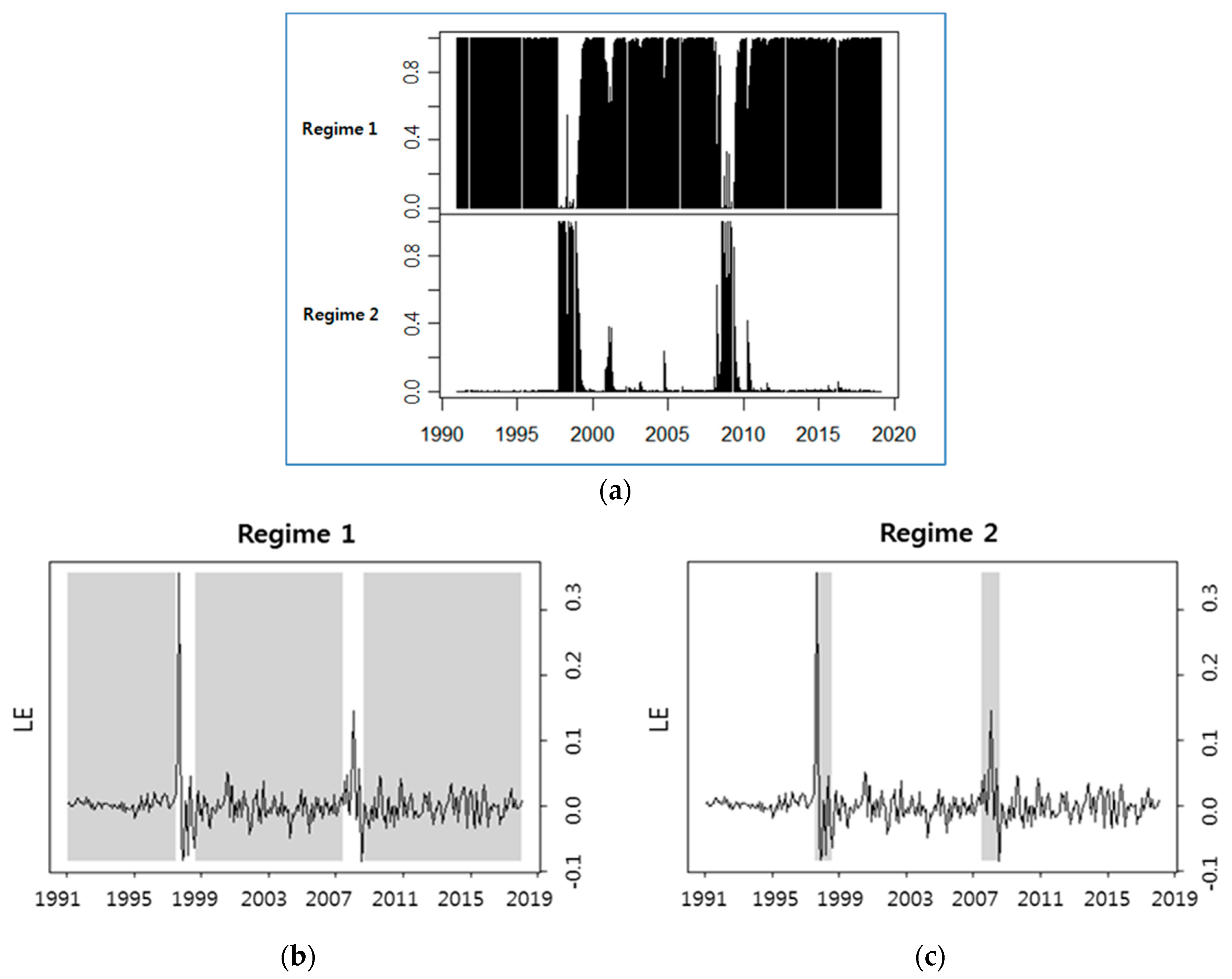
Each time point is grouped into one of the two regimes depending on its estimated filtered probability. At each time point $t$, the two filtered probabilities sum to 1. Figure 2a shows estimated probabilities of regimes. The upper plot presents the estimated probabilities of being in the regime 1 with low-volatility. The lower plot presents the estimated probabilities of being in the regime 2 with high-volatility, which consists of two periods. The first period lasted for 15 months from October 1997 to January 1999. The second period showed up for 11 months, once in April 2008 and then from August 2008 to May 2009.

Figure 2b,c shows volatilities of the raw data with grey area indicating regime 1 and regime 2, respectively, which are estimated based on the MRSM. Estimated high-volatility periods match the peaks around the Asian financial crisis in 1997 and the global financial crisis in 2008. Korean exchange rates markets suffered great instability during both periods.

We also examine how the explanatory variables influence the exchange rates in each regime, based on the selected best model 2(2p).

Table 3. Parameter estimates of the selected Markov two-regime switching model.

Regime	Parameters	Estimates	Standard Error
Regime 1 with low-volatility	Intercept $({\beta }_{01})$	−0.0001	0.0004
	$L{E}_{t-1}$$({\beta }_{11})$	0.2740	0.0563 ***
	$LOI{L}_t$$({\beta }_{21})$	−0.0230	0.0148
	$LRCP{I}_t$$({\beta }_{41})$	0.1058	0.2242
	Residual standard error	0.0148
	Multiple R2	0.1028
Regime 2 with high-volatility	Intercept $({\beta }_{02})$	0.0005	0.0108
	$L{E}_{t-1}$$\left({\beta }_{12}\right)$	−0.0462	0.2092
	$LOI{L}_t ({\beta }_{22})$	0.2181	0.1084 *
	$LRCP{I}_t$$({\beta }_{42})$	9.4279	2.2969 ***
	Residual standard error	0.0610
	Multiple R2	0.5025
Transition probabilities	$p_{12 }$	0.0811
	$p_{21}$	0.0081

Note: The response variable is exchange rate. The explanatory variables are oil prices and $CPI$. ${\beta }_{01}$ and ${\beta }_{02}$ are intercepts for regime 1 (low-volatility) and regime 2 (high-volatility). ${\beta }_{11}$ and ${\beta }_{12}$ are the coefficients of oil prices, ${\beta }_{21}$ and ${\beta }_{22}$ are the coefficients of $CPI$’s, ${\beta }_{p1}$ and ${\beta }_{p2}$ are the coefficients of (t-1) exchange rates, and ${\sigma }_1$ and ${\sigma }_2$ are the standard deviations of the two regimes. ***: significant at the 0.001 level. *: significant at the 0.05 level.

presents the parameter estimates for both regimes. The volatility of regime 2 with high-volatility (${\sigma }_2=0.0610$) was about four times that of regime 1 with low-volatility (${\sigma }_1=0.0148$). In regime 1 with low-volatility, Korean exchange rates were not significantly influenced by any of the explanatory variables, but had positive dependence on their auto-regressive term (p < 0.001). In regime 2 with high-volatility, the variable $LOIL$ positively influenced the exchange rates (p < 0.05) and the variable $LRCPI$ positively influenced the exchange rates to a much greater extent (p < 0.001). This shows that the exchange rates increase as oil prices or $CPI$s increase when the exchange rates markets are highly volatile. We observe that, in a highly volatile market, the exchange rates are significantly influenced by $CPI$s and oil prices but have no significant relationship with their auto-regressive terms. In a low-volatility market, only the auto-regressive terms are significant.

The each transition probabilities are $p_{11}=0.9189, p_{12}=0.0811, p_{21}=0.0081,$ and $p_{22}=0.9919$. The transition probability from the regime with low-volatility to the regime with high-volatility is about ten times that of the opposite case. The regime with low-volatility can much more easily transit to the regime with high-volatility when the explanatory variables change. This indicates that the Korean exchange rates market is, thus, vulnerable to external shocks.

Let us take a look at how much log-differentials of each explanatory variable can explain among the whole volatility of log-differentials of the exchange rates using the simple regression. The coefficient of determination $R^2$ in Table 2 shows the proportion of explained volatility compared to the total volatility of log-differentials of the exchange rates. In the regime with high-volatility of the model 1(3), we can see that the $CPI$s alone explains 43.6% of the exchange rates ($R^2$ = 0.436).

We extend this to the models with two explanatory variables. In the regime with high-volatility with model 2(2), the $CPI$s and oil prices together explain 49.0% of the exchange rates, a 5.4% increase in $R^2$. In addition, if the exchange rates auto-regressive term is added, as in model 2(2p), the $R^2$ value increases to 50.3%, an additional increase of 1.3%. All the coefficients of determination in the regime with low-volatility were quite small. Our model explains regimes with high-volatility much better than regimes with low-volatility. One interesting point is that the volatilities estimated in regimes with low-volatility, for all 30 of the models, were around 0.015.

4. Discussion

Let us compare the results with others which used the regime switching model. The previous regime switching model for oil prices and exchange rates of Korea includes Basher et al. [11]. In their findings, oil shocks had a statistically significant impact on exchange rates of Korea in the high-volatility regime, which is the same as ours. Their model assumed that exchange rates could be influenced not only by oil prices, but also by oil supply and global economic demand. Our model differs from theirs in that exchange rates are affected by price level, income, and interest rates as well as oil prices which are based on the monetary model of exchange rates determination. Nonetheless, the same conclusion was drawn that exchange rates are affected by oil prices in a high-volatility regime.

In

Table 4. Parameter estimates without the regime switching model.

Parameters	Estimates	Standard Error
Intercept $({\beta }_{01})$	−0.0003	0.0015
$L{E}_{t-1}({\beta }_{11})$	0.3969	0.0535 ***
$LOI{L}_t$$({\beta }_{21})$	0.0225	0.0226
$LRCP{I}_t$$({\beta }_{41})$	0.3442	0.3649 ***
Residual standard error	0.0266
Multiple R2	0.2475

Note: ***: significant at the 0.001 level.

, the auto-regression model without regime switching is also fitted for comparison. $R^2$ in the model is $0.247$, which is much less than 0.503 in the high-volatility regime. $LRCPI$ is significant (p < 0.01) but oil prices are not (p > 0.1). In the absence of regime switching, only $LRCPI$ and auto-regressive terms affect the Korean exchange rates. In other words, oil prices do not appear to affect the exchange rates, which is different from the results with MRSM. In the presence of Markov regime switching, oil prices significantly affect the exchange rates in the unstable regime. Thus, in models without Markov regime switching, the behavior in the stable regime overwhelms the behavior in the unstable regime. Korea has experienced two major economic crises, the Asian financial crisis and the global financial crisis, which are precisely detected by the MRSM. Therefore, it can be seen from this study that stable management of oil prices is essential for stabilizing exchange rates in these economic crises.

A long period time series data in this research often contains more than two different trends throughout the whole time period. We fit the two-regime MRSM, which estimates separate auto-regression models with AR (1) in each regime and the volatility state at each time point can switch between the two regimes according to the behavior of a Markov process.

Now, we check the assumptions of the errors, normality, and stationarity. The normality can be observed in the four residual plots in Figure 3. Plot (a) represents pooled residuals, where two distinctive high-volatile periods are observed, one around 1997–1998 and the other around 2008–2009. Plot (b) shows the normal quantile-quantile (QQ) plot of pooled residuals with p = 0.7998 from the Shapiro test. Separate QQ plots in the two regimes, plots (c) and (d), reveal more distinctive normality based on the Shapiro test (p = 0.0708 for regime 1 and p = 0.6241 for regime 2). The residuals in each regime show clear normal distribution, while pooled residuals seem to have outliers at both tails.

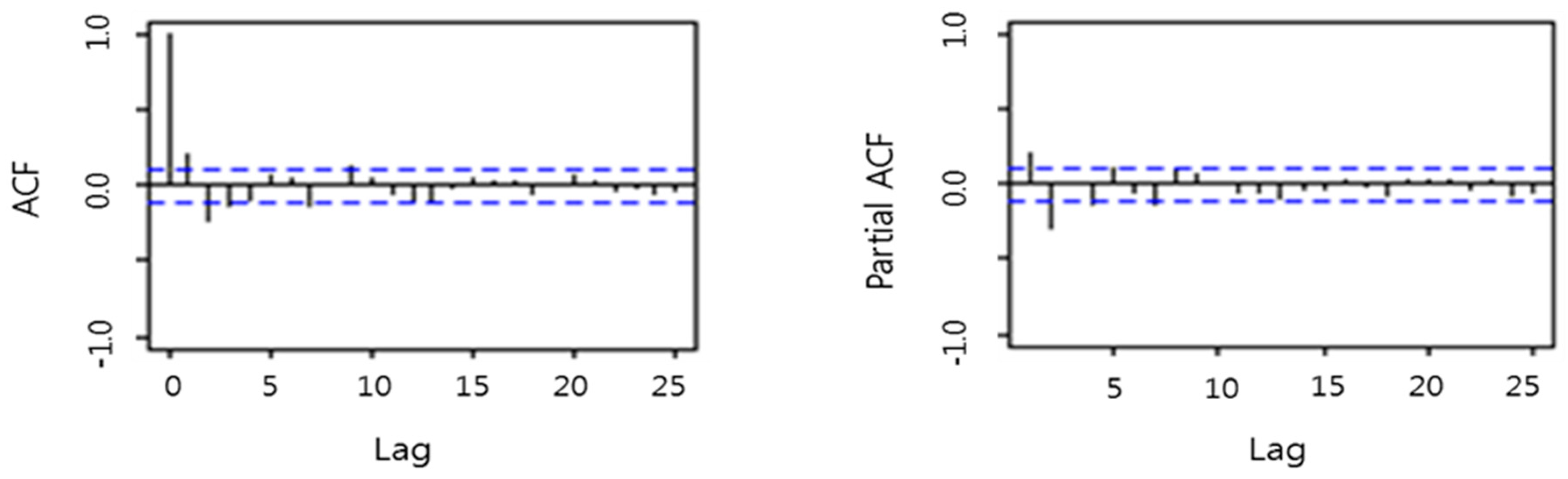
The stationarity can be observed by the autocorrelation function (ACF) and the partial autocorrelation function (PACF) of the residuals in Figure 4. Both ACFs and PACFs go to 0 as lag increases, which means stationarity of the residuals. Based on the Dickey–Fuller unit root test, the series $L{E}_{\mathrm{t}}$ is stationary (p = 0.0100), but the raw $Exchange Rat{e}_t$ before the transformation is not stationary (p = 0.4369). The adequacy of the selected model 2(2p) is confirmed by the normality based on QQ-plots and the Shapiro tests, and by the stationarity based on the Dickey–Fuller unit root test. All these goodness-of-fit results ensure relevance of selected explanatory variables in the model.

The parameter estimates for the MRSM were consistent in this study, even though they were known to be slightly inconsistent in each run as pointed out in the studies of Campbell [35], Kim, et al. [36], and Yuan [37]: “The unfiltered two-state Markov-switching model suffers estimation instability while the filtered model turns out to be temporally consistent” or “the Maximum Likelihood Estimator is inconsistent for regime-switching models in general”.

5. Conclusions

We analyzed the effects of oil prices, interest rates, $CPI$s, and $IPI$s on the regime shift behavior of the Korean exchange rates (against the USA.). This was the first attempt to study these issues, as far as we know. As a result of the MRSM, we detected regime shift behavior in the exchange rates, along with oil prices and major macroeconomic explanatory variables.

For this, we first set up a total of 30 models in consideration of the four variables to select the optimal MRSM, based on the $AIC$ and $MLL$. Finally, we selected the model that includes oil price, the difference of $CPI$s between the two countries (Korea and the USA), and the autoregressive term of the exchange rates.

Under the selected MRSM model, we found evidence to support the existence of two distinct regimes for all markets, one regime (1) with low-volatility and another regime (2) with high-volatility. The stable periods of regime 1 are much longer than the unstable periods of regime 2. The most unstable periods lasted for about two to three years. Regime 2, with high-volatility, occurred during the Asian financial crisis of 1997 and the global financial crisis of 2008–2009 in the Korean exchange rates market.

During the stable periods in the regime 1 with low-volatility, the Korean exchange rates were not significantly influenced by any of the explanatory variables, but had positive dependence on their auto-regressive terms at the 1% significance level. This implies that movements of changes of exchange rates are explained by their own previous movements, not by external variables during the stable periods. In the regime 2 with high-volatility, Korean exchange rates were significantly influenced by $CPI$s and oil prices, while their auto-regressive terms had no significant effect on the exchange rates. In other words, Korean exchange rates are more affected by external shocks than by their previous exchange rates during high volatile periods. As far as the exchange rates are concerned in the Korean market, $IPI$s and interest rates are not significant.

This result has very important implications about estimating the movements of changes of Korean exchange rates. Changes in oil prices significantly affect the prediction of Korean exchange rates during unstable periods. On the other hand, the consumer price level (compared to that of the US) has a much greater impact on the changes of exchange rates, compared to oil prices, in the Korean market. In other words, when the consumer price levels in Korea rise higher than those in the US, the movements of the changes of Korean exchange rates accordingly increase. Thus, maintaining stable consumer price levels in Korea contributes to the stabilization of Korean exchange rates.

When the major macroeconomic explanatory variables change, the regime with low-volatility could transit to the regime with high-volatility with 10 times higher transition probability than that of the opposite direction (i.e., from high to low). Thus, the Korean exchange rates market is vulnerable to external shock.

This study has the following limitations. Exchange rates are affected by both $CPI$s and $IPI$s, but both $CPI$s and $IPI$s can be also affected by exchange rates. However, this study does not consider this backward possibility. In other words, we only studied one-way analysis of $CPI$s and $IPI$s affecting exchange rates. In the future, this study can be extended to other countries which import and export oils to a great extent. New explanatory variables can be also added in future researches. Our results will provide valuable insights for Korean policy makers, about how to prepare for external shock, and also to Korean foreign exchange dealers, when they make decisions on foreign exchange speculation.