Multi-Frequency Single Loop Passivity-Based Control for LC-Filtered Stand-Alone Voltage Source Inverter

Abstract

The multi-frequency Passivity-Based Control (PBC) has been successfully applied in L-filtered power converters. For an LC-filtered stand-alone voltage source inverter (VSI), the mathematical model is second-order, where two state variables are used in modeling and control in conventional multi-frequency PBC controller, complicating the controller design and increasing the occupied resources both in hardware and software. In order to simplify the controller design and save the resources as well as the cost, a control scheme called multi-frequency single-loop PBC is proposed for the LC-filtered stand-alone VSI in this paper. The feasibility of the proposed control strategy is verified through the experimental results on a 3-phase/110 V/6 kW prototype.

1. Introduction

Whether in traditional or modern applications, grid-tied inverters are widely utilized in industry [1]. Furthermore, stand-alone voltage source inverters (VSIs) as an another power converter are also widely adopted in various industrial situations, such as uninterrupted power supply (UPS) systems [2,3,4], AC power supply system [5,6,7], grid simulator systems [8,9], power electronic transformer systems [10,11] and etc. Therefore, to promote the performance of VSI is of great importance for the above applications. The output voltage waveform of a high-performance VSI must be sinusoidal, with specified frequency and amplitude, low total harmonic distortion (THD), especially under the condition of nonlinear loads [4]. In addition to above requirements, a VSI system must have good disturbance rejection, excellent voltage regulation, and fast dynamic response.

To improve the aforementioned performance indexes, a number of control algorithms, such as deadbeat control [12,13], repetitive control [14,15], proportional-resonant with damping control method [1,16,17,18], sliding mode control [3,19,20], hysteresis control [21], predictive control [22,23], adaptive control [24], optimal control [25], and passivity-based control (PBC) [26], have been proposed for VSIs. Among these control techniques, the PBC is a hybrid control scheme combined with the instruction predicting feedforward control, the disturbance feedforward control, the decoupling control, and the negative feedback control. The emergence of the PBC technique has generated a new idea of the controller design for nonlinear systems [27,28], which has attracted the attention of many scholars, and the application of PBC on power electronics can be found in [27,28,29,30,31,32,33,34,35,36,37,38,39].

Essentially, the PBC controller is designed from the perspective of system structure and energy. For example, as introduced in [29], the ac-side currents of the converter were well controlled by the inner loop of the PBC together with the outer loop of the PI regulator to control dc-side voltage. The dynamic damping injection for the PBC had been studied in [34] and [35], respectively. In [36] and [37], the model of a Port-Controlled Hamiltonian system with Dissipation (PCHD) for converters with different structures was established, and the PBC controller design of the model was realized through interconnection and damping distribution.

Although the aforementioned research had proven that the application of PBC controllers in nonlinear systems is feasible and the advantages of better dynamic performance and stronger robustness can be achieved, the Conventional PBC (C-PBC) controller for the second-order system like LC-filtered stand-alone VSI is a double-loop controller, where two state variables have to be adopted. Therefore, more sensors and software resource must be occupied to realize the control scheme and more control parameters must be selected.

In view of the demerit of C-PBC controller, a modified multi-frequency single loop PBC controller is proposed for LC-filtered VSI, where the double-loop controller can be simplified as a single loop controller (only one control parameter), which saves a lot of calculation time, as well as the sensor costs. Note that zero steady-state error can be also achieved by using an inserted dynamic dissipation term.

The paper is organized as follows. In Section 2, the mathematical model and C-PBC controller are presented, and the disadvantages of this method are studied. Then, a modified multi-frequency single loop based PBC controller is proposed in Section 3. The experimental results are shown in Section 4 to prove that the proposed control strategy is feasible. Finally, there is a conclusion in Section 5.

2. Mathematical Model and Conventional PBC of LC-Filtered VSI

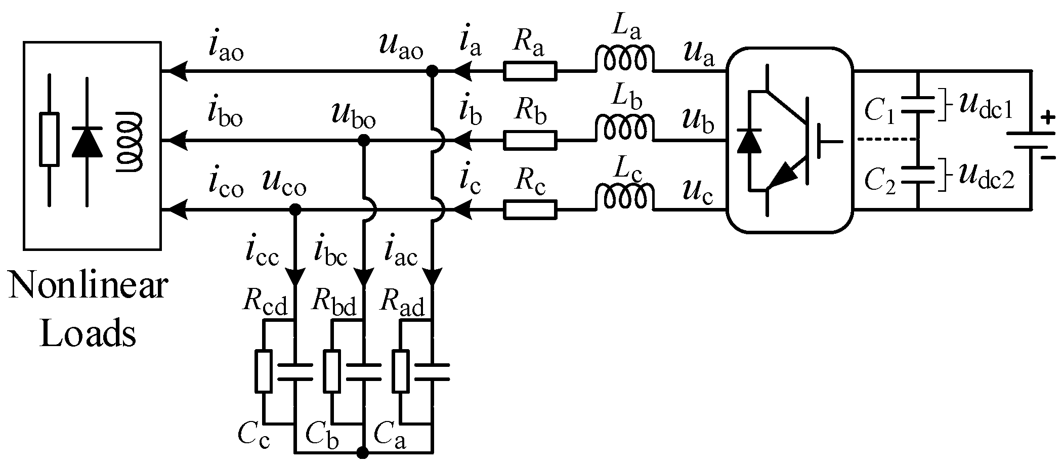
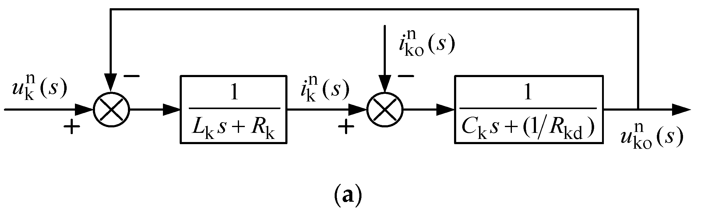
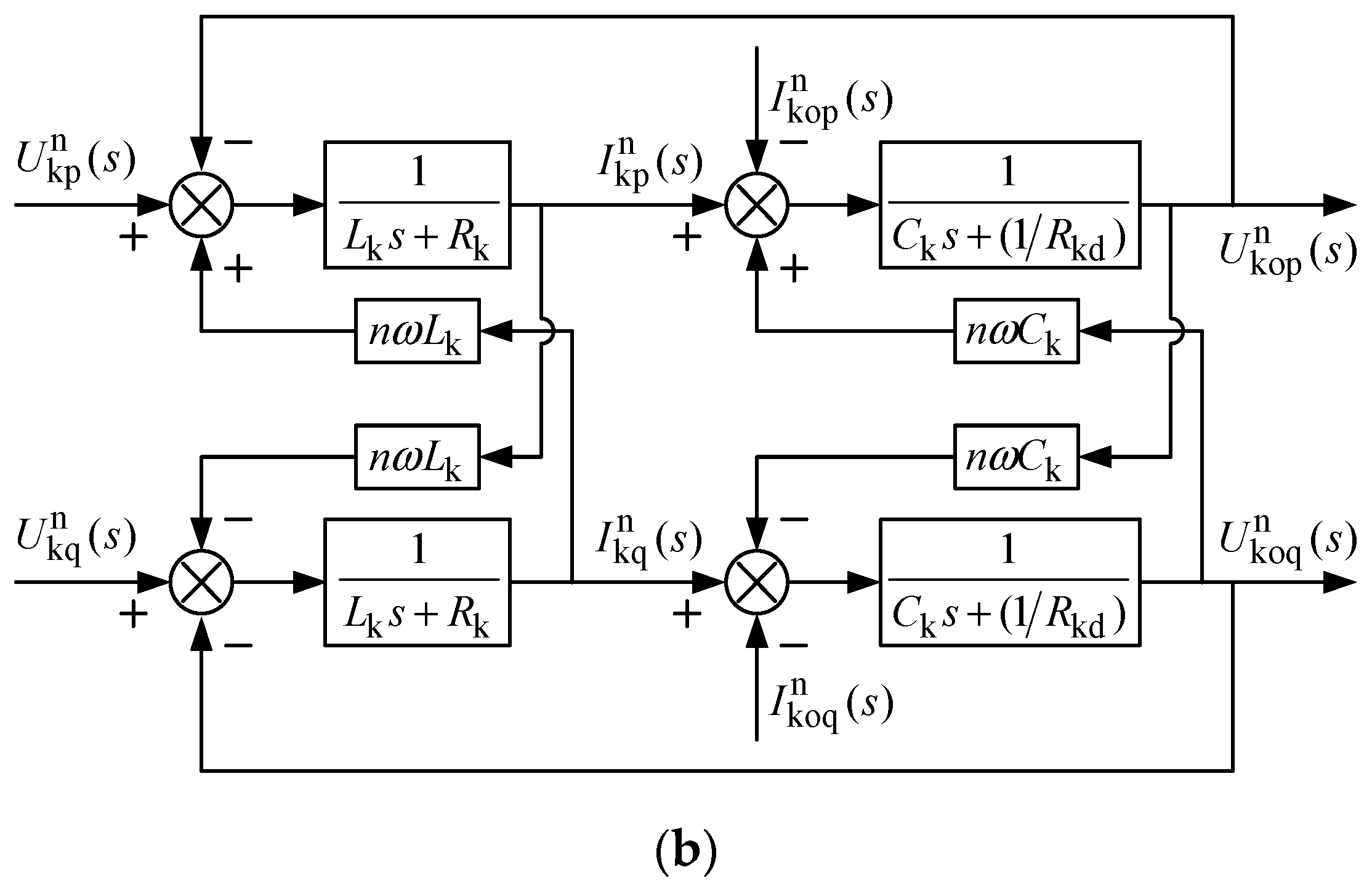
2.1. Mathematical Model of LC-Filtered VSI

Typical structure of stand-alone VSI with nonlinear loads is shown in Figure 1, where the inverter is a three-level neutral point clamped (NPC) inverter. In Figure 1, C₁ and C₂ at DC side are the DC support capacitors. u_k is the three-phase voltage output from the converter; L_k is the filter inductor; R_k is the line impedance; i_k is the inductor current; C_k is the filter capacitor; R_kd is the equivalent parallel resistance of the filter capacitor and the filter damping resistance; i_kc is the filter capacitor current; u_ko is the filter capacitor voltage; and i_ko is the load current. k = phase-a, b, and c. It can be obtained from Figure 1,

$$\{\begin{array}{l}{L}_k\frac{d{i}_{\mathrm{k}}}{dt}+R_{\mathrm{k}}{i}_{\mathrm{k}}=u_{\mathrm{k}}-u_{\mathrm{ko}}\\ C_k\frac{d{u}_{\mathrm{ko}}}{dt}+\frac{u_{\mathrm{ko}}}{R_{\mathrm{kd}}}=i_{\mathrm{kc}}=i_{\mathrm{k}}-i_{\mathrm{ko}}\end{array}$$

(1)

where u_k = f_k(S_a, S_b, S_c, u_dc1, u_dc2), the function f_k can be calculated by using a modulation strategy, such as SPWM and SVPWM, and S_a, S_b, and S_c are the switch functions.

The fast Fourier transform (FFT) method is utilized to achieve a better control performance, and the main advantages of this modeling method include: (1) it can realize the frequency spectral decomposition of the AC mathematical model of the series converter, which is convenient for the control at selected frequencies; and (2) it can realize the transformation from the AC model to the DC model, which is convenient for DC signal control. In addition, this method can overcome some shortcomings of the conventional modeling method (modelling in d-q axis). For example, [40] had pointed out that it is only suitable for the modeling of three-phase systems, and the phase-to-phase coupling occurs during the modeling process, which is inconvenient to achieve individual phase control. During the modeling, the parameters of each phase of the three-phase system, such as output filter inductance, capacitance, and line resistance, are assumed to be symmetric.

Here, ${\mathsf{\Gamma }}_{\mathrm{k}-{\mathrm{k}}_{\mathrm{q}}^{\mathrm{p}}}^{\mathrm{n}}$ is denoted as the positive Fourier transform matrix of phase-k of the system, and ${\mathsf{\Gamma }}_{{\mathrm{k}}_{\mathrm{q}}^{\mathrm{p}}-\mathrm{k}}^{\mathrm{n}}$ as the inverse Fourier transform matrix, as shown in Equation (2),where, k = a, b, c, and λ = 0, -1, 1, respectively. x(t) is any finite bandwidth periodic signal, whose period is T, and the bandwidth is from the fundamental angle frequency ω to N_mω,

$$\{\begin{array}{l}{\mathsf{\Gamma }}_{\mathrm{k}-{\mathrm{k}}_{\mathrm{q}}^{\mathrm{p}}}^{\mathrm{n}}=\left[\begin{array}{c}{X}_{\mathrm{p}}\\ X_{\mathrm{q}}\end{array}\right]=\frac{2}{T}\left[\begin{array}{c}{\displaystyle {\int }_0^{T}x(t)\sin (n\omega t+\frac{2\lambda }{3}\pi )dt}\\ {\displaystyle {\int }_0^{T}x(t)\cos (n\omega t+\frac{2\lambda }{3}\pi )dt}\end{array}\right]\\ {\mathsf{\Gamma }}_{{\mathrm{k}}_{\mathrm{q}}^{\mathrm{p}}-\mathrm{k}}^{\mathrm{n}}=\left[\begin{array}{cc}\sin (n\omega t+\frac{2\lambda }{3}\pi )& \cos (n\omega t+\frac{2\lambda }{3}\pi )\end{array}\right]\end{array}$$

(2)

Note that, Equation (1) can be also decomposed into the sum of nth order harmonic components as follows,

$$\{\begin{array}{l}{L}_{\mathrm{k}}{\displaystyle \sum _{n=1}^{n=N_{\mathrm{m}}}\frac{d{i}_{\mathrm{k}}^{\mathrm{n}}}{dt}}+R_{\mathrm{k}}{\displaystyle \sum _{n=1}^{n=N_{\mathrm{m}}}{i}_{\mathrm{k}}^{\mathrm{n}}}={\displaystyle \sum _{n=1}^{n=N_{\mathrm{m}}}(u_{\mathrm{k}}^{\mathrm{n}}-u_{\mathrm{k}\mathrm{o}}^{\mathrm{n}})}\\ C_{\mathrm{k}}{\displaystyle \sum _{n=1}^{n=N_{\mathrm{m}}}\frac{d{u}_{\mathrm{k}\mathrm{o}}^{\mathrm{n}}}{dt}}+\frac{1}{R_{\mathrm{kd}}}{\displaystyle \sum _{n=1}^{n=N_{\mathrm{m}}}{u}_{\mathrm{ko}}^{\mathrm{n}}}={\displaystyle \sum _{n=1}^{n=N_{\mathrm{m}}}(i_{\mathrm{k}}^{\mathrm{n}}-i_{\mathrm{k}\mathrm{o}}^{\mathrm{n}})}\end{array}$$

(3)

where n = 1, 2,…, N_m, and N_m are the maximum harmonic order; i_kⁿ is the nth harmonic component of the inductive current; u_kⁿ is the nth harmonic component of the PWM voltage output from the converter; u_koⁿ is the nth harmonic component of the filter capacitor voltage, and i_koⁿ is the nth harmonic component of the output current (or load current). The Fourier transform process from the nth harmonic AC to DC model of each phase can be represented by the transfer function block diagram shown in Figure 2.

For the nth harmonic system, Equation (3) can be rewritten using FFT transformation as,

$$\{\begin{array}{c}{L}_k\frac{d{I}_{kp}^n}{dt}+R_{\mathrm{k}}{I}_{kp}^n-\omega L_k{I}_{kq}^n=U_{kp}^n-U_{kop}^n\\ L_k\frac{d{I}_{kq}^n}{dt}+R_{\mathrm{k}}{I}_{kq}^n+\omega L_k{I}_{kq}^n=U_{kq}^n-U_{koq}^n\\ C_k\frac{d{U}_{kop}^n}{dt}+\frac{U_{kop}^n}{R_{\mathrm{kd}}}-\omega C_k{U}_{koq}^n=I_{kp}^n-I_{kop}^n\\ C_k\frac{d{U}_{koq}^n}{dt}+\frac{U_{koq}^n}{R_{\mathrm{kd}}}+\omega C_k{U}_{kop}^n=I_{kq}^n-I_{koq}^n\end{array}$$

(4)

The Euler Lagrange (EL) model is adopted to describe the system, and Equation (4) can be rewritten in EL form as,

$$M\dot{x}+Jx+Rx=u$$

(5)

where $M=\left(\begin{array}{cccc}{L}_k& 0& 0& 0\\ 0& L_k& 0& 0\\ 0& 0& C_k& 0\\ 0& 0& 0& C_k\end{array}\right)$, $R=\left(\begin{array}{cccc}{R}_k& 0& 0& 0\\ 0& R_k& 0& 0\\ 0& 0& \raisebox{1ex}{$1$}\!\left/ \!\raisebox{-1ex}{$R_{kd}$}\right.& 0\\ 0& 0& 0& \raisebox{1ex}{$1$}\!\left/ \!\raisebox{-1ex}{$R_{kd}$}\right.\end{array}\right)$, $J=\left(\begin{array}{cccc}0& -n\omega L_k& 1& 0\\ n\omega L_k& 0& 0& 1\\ -1& 0& 0& -n\omega C_k\\ 0& -1& n\omega C_k& 0\end{array}\right)$, $x=\left(\begin{array}{c}{I}_{kp}^n\\ I_{kq}^n\\ U_{kop}^n\\ U_{koq}^n\end{array}\right)$, and $u=\left(\begin{array}{c}{U}_{kp}^n-U_{kop}^n\\ U_{kq}^n-U_{koq}^n\\ I_{kp}^n-I_{kop}^n\\ I_{kq}^n-I_{koq}^n\end{array}\right)$.

2.2. C-PBC Controller for LC-Filtered VSI

The passivity of the LC-filtered grid-tied inverter (GTI) is proven in [39], so it is omitted here. Define the reference vector as x* = (I_kpⁿ* I_kqⁿ* U_kopⁿ* U_koqⁿ*)^T, the error vector is x_e = x* − x, then the error EL model can be obtained as

$$M{\dot{x}}_e+J{x}_e+R{x}_e=M{\dot{x}}^{*}+J{x}^{*}+R{x}^{*}-u$$

(6)

In steady state, x_e equals to zero. In order to accelerate the speed of convergence, a dissipation matrix r_d is added to the error system. The dissipation matrix and new dissipation matrix is obtained as

$$r_d=diag\left(\begin{array}{cccc}{r}_2& r_2& r_1& r_1\end{array}\right),R_{new}=R+r_d$$

(7)

So, the new error EL equation is obtained as

$$M{\dot{x}}_e+J{x}_e+R_{new}{x}_e=M{\dot{x}}^{*}+J{x}^{*}+R{x}^{*}+r_d{x}_e-u$$

(8)

When x_e is equal to zero, the conventional PBC control law $u$ can be obtained,

$$u=M{\dot{x}}^{*}+J{x}^{*}+R{x}^{*}+r_d{x}_e$$

(9)

According to Equation (9), the C-PBC control structure is depicted in Figure 3.

From Figure 3, it can be seen that there are two control loops to track two state variables in the C-PBC controller. Therefore, at least six sensors (current and voltage) must be adopted in the three-phase system to achieve the control scheme and more software resource must be occupied. In order to simplify the controller and save costs, a multi-frequency single loop controller is proposed, which is described in detail in the next section. Note that, the inertia term $\frac{1}{T_{\omega }s+1}$ in Figure 2 represents the time delay caused by FFT.

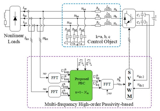
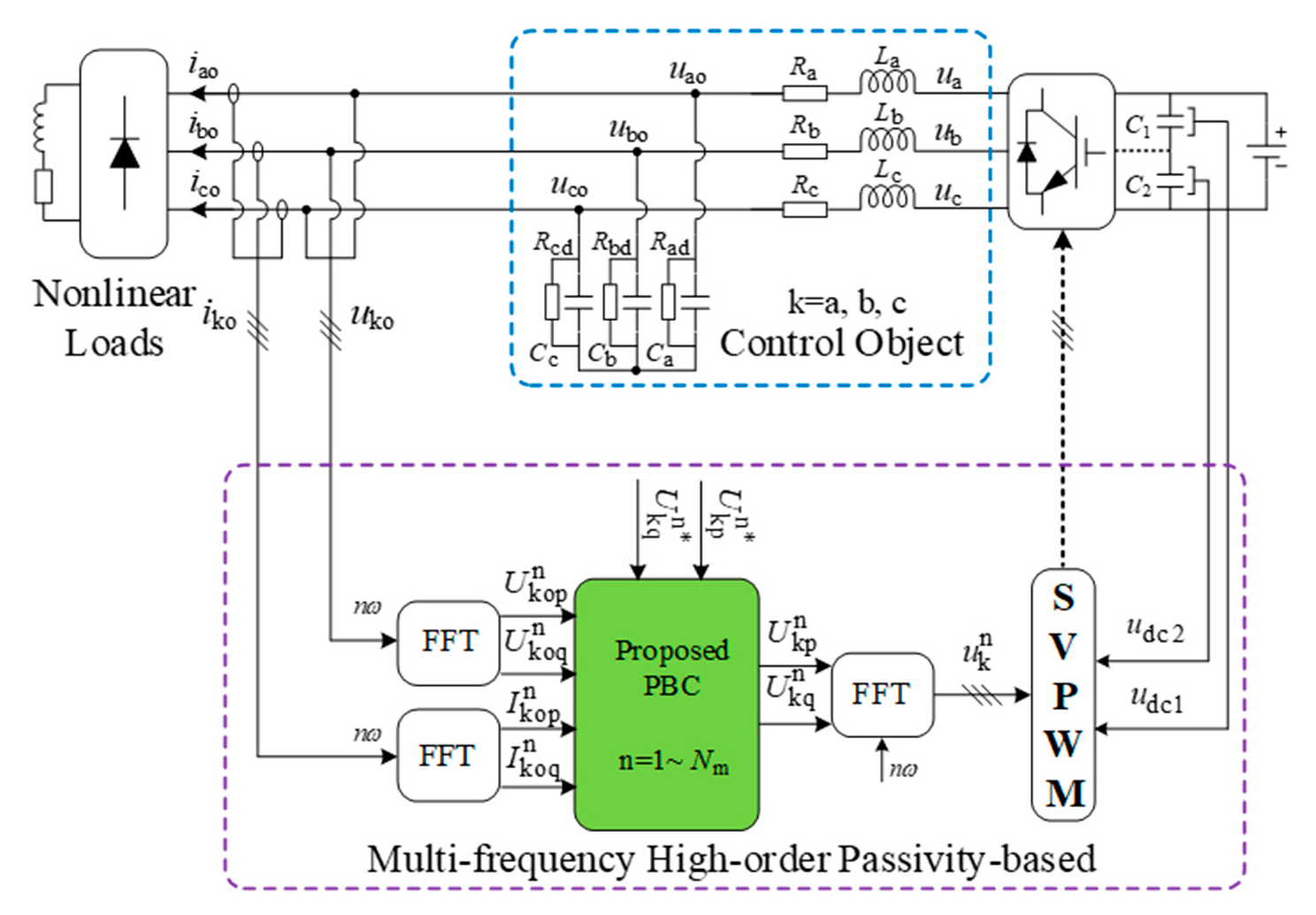
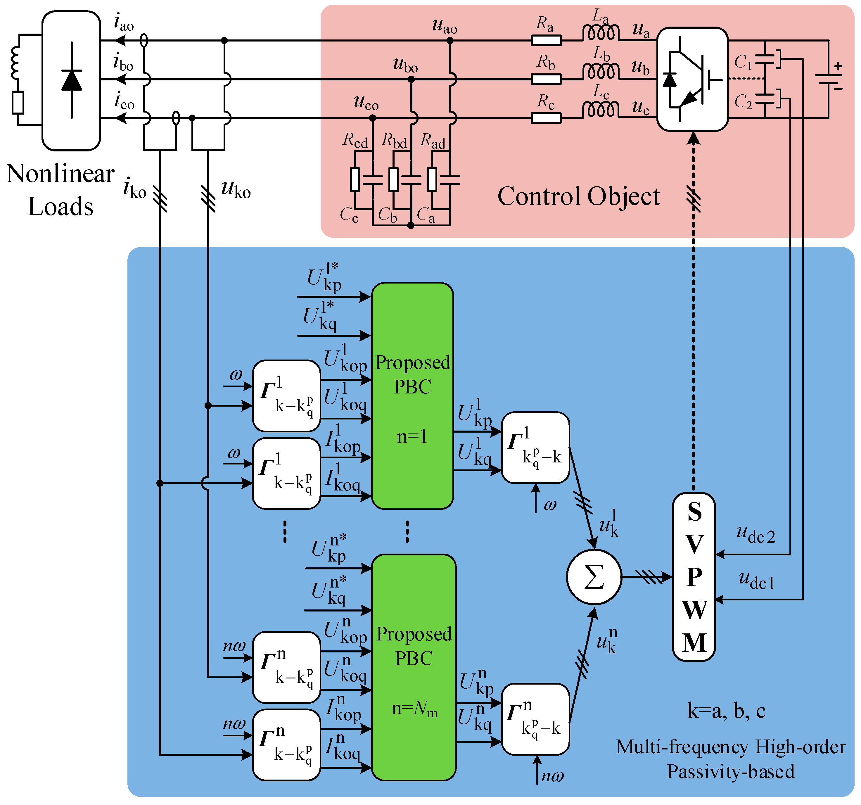
3. Modified Multi-Frequency Single Loop PBC Controller

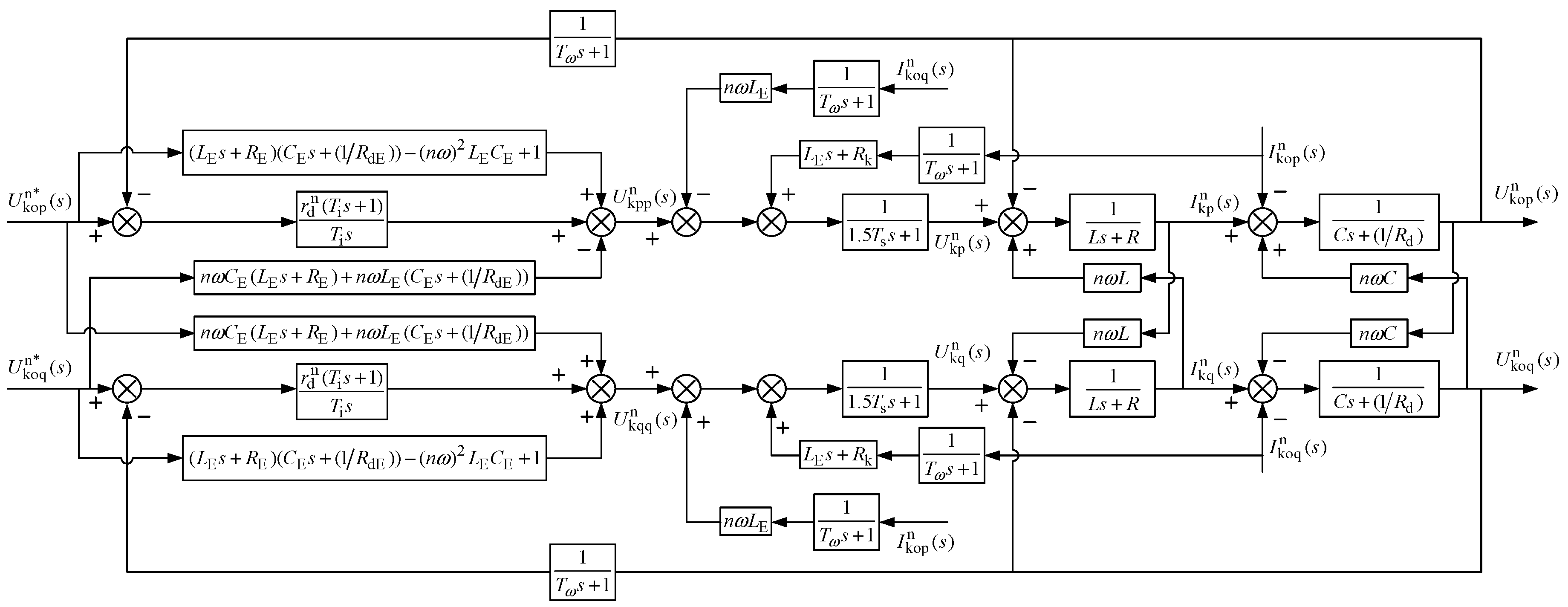
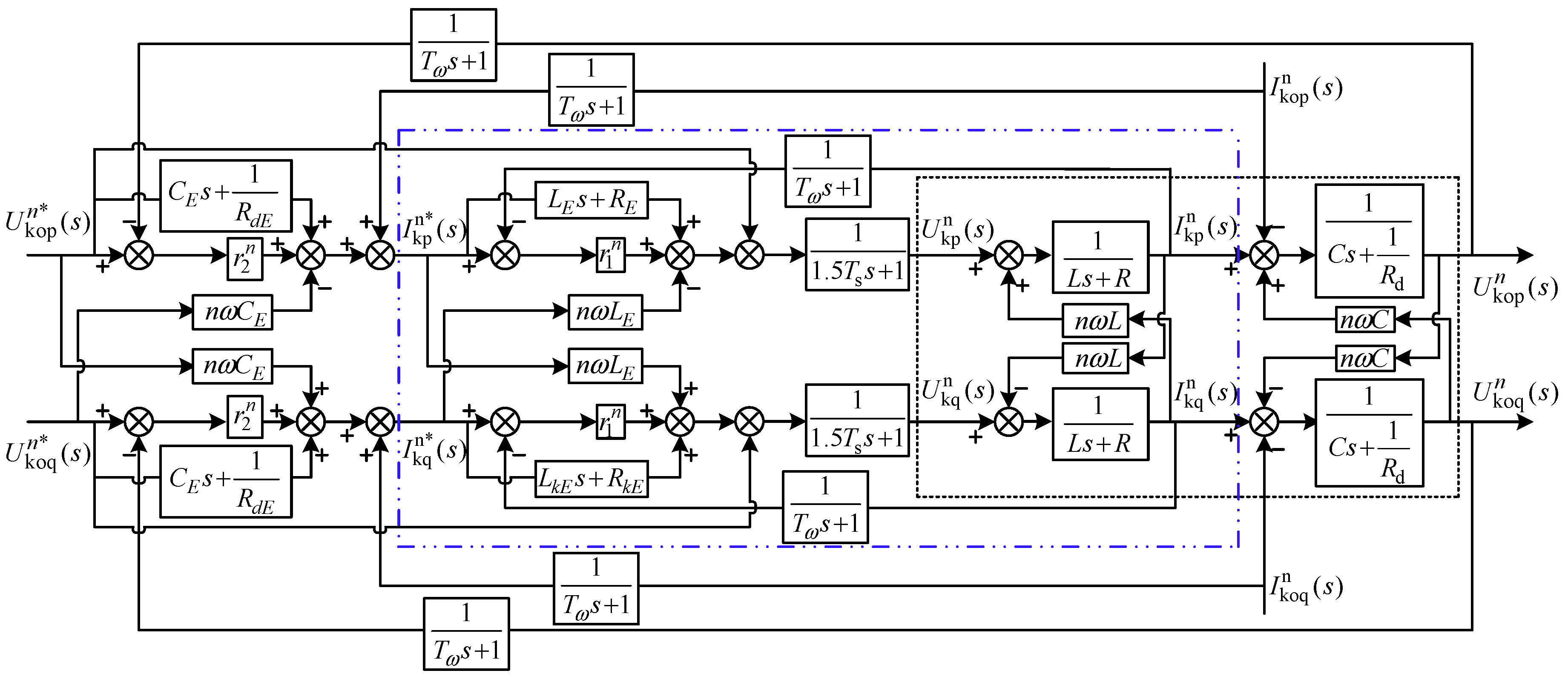
3.1. Multi-Frequency Single Loop PBC Control Law

Equation (4) also can be rewritten as

$$\{\begin{array}{l}{\mathit{M}}_{L\mathrm{k}}{\dot{\mathit{x}}}_{I\mathrm{k}}^{\mathrm{n}}+{\mathit{J}}_{L\mathrm{k}}{\mathit{x}}_{I\mathrm{k}}^{\mathrm{n}}+{\mathit{R}}_{\mathrm{k}}{\mathit{x}}_{I\mathrm{k}}^{\mathrm{n}}={\mathit{U}}_{\mathrm{k}}^{\mathrm{n}}-{\mathit{x}}_{\mathit{U}\mathrm{k}}^{\mathrm{n}}\\ {\mathit{M}}_{C\mathrm{k}}{\dot{\mathit{x}}}_{\mathit{U}\mathrm{k}}^{\mathrm{n}}+{\mathit{J}}_{C\mathrm{k}}{\mathit{x}}_{\mathit{U}\mathrm{k}}^{\mathrm{n}}+{\mathit{R}}_{\mathrm{kd}}{\mathit{x}}_{\mathit{U}\mathrm{k}}^{\mathrm{n}}={\mathit{x}}_{I\mathrm{k}}^{\mathrm{n}}-{\mathit{I}}_{\mathrm{ko}}^{\mathrm{n}}\end{array}$$

(10)

As can be seen from (10), the system variables including ${\mathit{x}}_{\mathrm{I}\mathrm{k}}^{\mathrm{n}}$ and ${\mathit{x}}_{U\mathrm{k}}^{\mathrm{n}}$, while ${\mathit{x}}_{I\mathrm{k}}^{\mathrm{n}}$ is a temporary variable and ${\mathit{I}}_{\mathrm{k}\mathrm{o}}^{\mathrm{n}}$ is a disturbance variable. Therefore, the two equations in Equation (9) can be combined to a new EL equation as

$${\mathit{M}}_{\mathrm{k}}{\ddot{\mathit{x}}}_{\mathrm{k}}^{\mathrm{n}}+\left({\mathit{J}}_{1\mathrm{k}}{\dot{\mathit{x}}}_{\mathrm{k}}^{\mathrm{n}}+{\mathit{J}}_{2\mathrm{k}}{\mathit{x}}_{\mathrm{k}}^{\mathrm{n}}\right)+{\mathit{D}}_{\mathrm{k}}{\dot{\mathit{x}}}_{\mathrm{k}}^{\mathrm{n}}+{\mathit{K}}_{\mathrm{k}}^{\mathrm{n}}{\mathit{x}}_{\mathrm{k}}^{\mathrm{n}}+{\mathit{N}}_{\mathrm{k}}^{\mathrm{n}}={\mathit{u}}_{\mathrm{k}}^{\mathrm{n}}$$

(11)

where, ${\mathit{M}}_{\mathrm{k}}=\left(\begin{array}{cc}{L}_{\mathrm{k}}{C}_{\mathrm{k}}& 0\\ 0& L_{\mathrm{k}}{C}_{\mathrm{k}}\end{array}\right),{\mathit{J}}_{1\mathrm{k}}=\left(\begin{array}{cc}0& -2n\omega L_{\mathrm{k}}{C}_{\mathrm{k}}\\ 2n\omega L_{\mathrm{k}}{C}_{\mathrm{k}}& 0\end{array}\right),{\mathit{J}}_{2\mathrm{k}}=\left(\begin{array}{cc}0& -(n\omega R_{\mathrm{k}}{C}_{\mathrm{k}}+\frac{n\omega L_{\mathrm{k}}}{R_{\mathrm{kd}}})\\ n\omega R_{\mathrm{k}}{C}_{\mathrm{k}}+\frac{n\omega L_{\mathrm{k}}}{R_{\mathrm{kd}}}& 0\end{array}\right),$ ${\mathit{D}}_{\mathrm{k}}=\left(\begin{array}{cc}{R}_{\mathrm{k}}{C}_{\mathrm{k}}+\frac{L_{\mathrm{k}}}{R_{\mathrm{kd}}}& 0\\ 0& R_{\mathrm{k}}{C}_{\mathrm{k}}+\frac{L_{\mathrm{k}}}{R_{\mathrm{kd}}}\end{array}\right),{\mathit{K}}_{\mathrm{k}}^{\mathrm{n}}=\left(\begin{array}{cc}1-{(n\omega )}^2{L}_{\mathrm{k}}{C}_{\mathrm{k}}+\frac{R_{\mathrm{k}}}{R_{\mathrm{kd}}}& 0\\ 0& 1-{(n\omega )}^2{L}_{\mathrm{k}}{C}_{\mathrm{k}}+\frac{R_{\mathrm{k}}}{R_{\mathrm{kd}}}\end{array}\right),$ ${\mathit{N}}_{\mathrm{k}}^{\mathrm{n}}=\left(\begin{array}{cc}{L}_{\mathrm{k}}& 0\\ 0& L_{\mathrm{k}}\end{array}\right)\left(\begin{array}{c}\frac{d}{dt}{I}_{\mathrm{k}\mathrm{o}\mathrm{p}}^{\mathrm{n}}\\ \frac{d}{dt}{I}_{\mathrm{k}\mathrm{o}\mathrm{q}}^{\mathrm{n}}\end{array}\right)+\left(\begin{array}{cc}{R}_{\mathrm{k}}& -n\omega L_{\mathrm{k}}\\ n\omega L_{\mathrm{k}}& R_{\mathrm{k}}\end{array}\right)\left(\begin{array}{c}{I}_{\mathrm{k}\mathrm{o}\mathrm{p}}^{\mathrm{n}}\\ I_{\mathrm{k}\mathrm{o}\mathrm{q}}^{\mathrm{n}}\end{array}\right),$ ${\mathit{x}}_{\mathrm{k}}^n=\left(\begin{array}{c}{U}_{\mathrm{k}\mathrm{o}\mathrm{p}}^{\mathrm{n}}\\ U_{\mathrm{k}\mathrm{o}\mathrm{q}}^{\mathrm{n}}\end{array}\right),$ and ${\mathit{u}}_{\mathrm{k}}^{\mathrm{n}}=\left(\begin{array}{c}{U}_{\mathrm{k}p}^n\\ U_{\mathrm{k}q}^n\end{array}\right).$

It can be seen from Equation (11) that the EL equation of the system becomes a higher-order equation. Here, select a stored (Lyapunov) function

$$H_{\mathrm{k}}^{\mathrm{n}}=\frac{1}{2}{({\dot{\mathit{x}}}_{\mathrm{k}}^{\mathrm{n}})}^{\mathrm{T}}{\mathit{M}}_{\mathrm{k}}{\dot{\mathit{x}}}_{\mathrm{k}}^{\mathrm{n}}+\frac{1}{2}{({\mathit{x}}_{\mathrm{k}}^{\mathrm{n}})}^{\mathrm{T}}{\mathit{K}}_{\mathrm{k}}{\mathit{x}}_{\mathrm{k}}^{\mathrm{n}}$$

(12)

Taking the time derivative of (12), it yields

$${\dot{H}}_{\mathrm{k}}^{\mathrm{n}}={({\dot{\mathit{x}}}_{\mathrm{k}}^{\mathrm{n}})}^{\mathrm{T}}{\mathit{u}}_{\mathrm{k}}^{\mathrm{n}}-{({\dot{\mathit{x}}}_{\mathrm{k}}^{\mathrm{n}})}^{\mathrm{T}}{\mathit{D}}_{\mathrm{k}}{\dot{\mathit{x}}}_{\mathrm{k}}^{\mathrm{n}}-{({\dot{\mathit{x}}}_{\mathrm{k}}^{\mathrm{n}})}^{\mathrm{T}}{\mathit{N}}_{\mathrm{k}}^{\mathrm{n}}<{({\dot{\mathit{x}}}_{\mathrm{k}}^{\mathrm{n}})}^{\mathrm{T}}({\mathit{u}}_{\mathrm{k}}^{\mathrm{n}}-{\mathit{N}}_{\mathrm{k}}^{\mathrm{n}})$$

(13)

According to the passive condition, it can be seen from (13), the system at harmonic high-order is strictly passive. Therefore, the PBC can be designed on high-order nth harmonic system.

Redefine the reference vector and error vector of the nth harmonic voltage of the filter capacitor as

$${\mathit{x}}_{\mathrm{k}}^{\mathrm{n}*}={[\begin{array}{cc}{\mathit{U}}_{\mathrm{k}op}^{\mathrm{n}\ast }& {\mathit{U}}_{\mathrm{k}oq}^{\mathrm{n}\ast }\end{array}]}^T,{\mathit{x}}_{\mathrm{k}e}^{\mathrm{n}}={\mathit{x}}_{\mathrm{k}}^{\mathrm{n}\ast }-{\mathit{x}}_{\mathrm{k}}^{\mathrm{n}}$$

(14)

If the Equation (14) is taken into Equation (11), the higher-order EL equation of the nth harmonic error system of the series converter can be obtained.

$$\begin{array}{l}{\mathit{M}}_{\mathrm{k}}{\ddot{\mathit{x}}}_{\mathrm{k}e}^{\mathrm{n}}+({\mathit{J}}_{1\mathrm{k}}^{\mathrm{n}}{\dot{\mathit{x}}}_{\mathrm{k}e}^{\mathrm{n}}+{\mathit{J}}_{2\mathrm{k}}^{\mathrm{n}}{\mathit{x}}_{\mathrm{k}e}^{\mathrm{n}})+{\mathit{D}}_{\mathrm{k}}{\dot{\mathit{x}}}_{\mathrm{k}e}^{\mathrm{n}}+{\mathit{K}}_{\mathrm{k}}^{\mathrm{n}}{\mathit{x}}_{\mathrm{ke}}^{\mathrm{n}}\\ ={\mathit{M}}_{\mathrm{k}}{\ddot{\mathit{x}}}_{\mathrm{k}}^{\mathrm{n}*}+({\mathit{J}}_{1\mathrm{k}}^{\mathrm{n}}{\dot{\mathit{x}}}_{\mathrm{k}}^{\mathrm{n}*}+{\mathit{J}}_{2\mathrm{k}}^{\mathrm{n}}{\mathit{x}}_{\mathrm{k}}^{\mathrm{n}*})+{\mathit{D}}_{\mathrm{k}}{\dot{\mathit{x}}}_{\mathrm{k}}^{\mathrm{n}*}+{\mathit{K}}_{\mathrm{k}}^{\mathrm{n}}{\mathit{x}}_{\mathrm{k}}^{\mathrm{n}*}+{\mathit{N}}_{\mathrm{k}}^{\mathrm{n}}-{\mathit{u}}_{\mathrm{k}}^{\mathrm{n}}\end{array}$$

(15)

Similarly, an additional dissipation term should be added on both sides of (15), note that, the dissipation term in conventional PBC is static, where the steady-state error will occur if the parameters drift [38]. In order to achieve zero steady-state error, a modified dissipation term named dynamic dissipation term is adopted and it can be written as

$${\mathit{r}}_{new}={\mathit{r}}_{\mathrm{kd}}^{\mathrm{n}}{\mathit{x}}_{\mathrm{ke}}^{\mathrm{n}}+{\mathit{k}}_{\mathrm{ki}}^{\mathrm{n}}{\displaystyle {\int }_0^{T_i}{\mathit{x}}_{\mathrm{ke}}^{\mathrm{n}}dt}$$

(16)

where, ${\mathit{r}}_{\mathrm{kd}}^{\mathrm{n}}=diag(r_{\mathrm{kd}}^{\mathrm{n}}>0,r_{\mathrm{kd}}^{\mathrm{n}}>0),{\mathit{k}}_{\mathrm{ki}}^{\mathrm{n}}=diag(k_{\mathrm{i}}^{\mathrm{n}}>0,k_{\mathrm{i}}^{\mathrm{n}}>0)$. And (16) should be satisfied

$$1-{(n\omega )}^2{L}_{\mathrm{k}}{C}_{\mathrm{k}}+(R_{\mathrm{k}}/R_{\mathrm{kd}})+r_{\mathrm{kd}}^{\mathrm{n}}>0$$

(17)

Then, the new error EL model can be obtained,

$$\begin{array}{l}{\mathit{M}}_{\mathrm{k}}{\ddot{\mathit{x}}}_{\mathrm{k}\mathrm{e}}^{\mathrm{n}}+({\mathit{J}}_{1\mathrm{k}}^{\mathrm{n}}{\dot{\mathit{x}}}_{\mathrm{k}\mathrm{e}}^{\mathrm{n}}+{\mathit{J}}_{2\mathrm{k}}^{\mathrm{n}}{\mathit{x}}_{\mathrm{k}\mathrm{e}}^{\mathrm{n}})+{\mathit{D}}_{\mathrm{k}}{\dot{\mathit{x}}}_{\mathrm{k}\mathrm{e}}^{\mathrm{n}}+({\mathit{K}}_{\mathrm{k}}^{\mathrm{n}}+{\mathit{r}}_{\mathrm{kd}}^{\mathrm{n}}){\mathit{x}}_{\mathrm{k}\mathrm{e}}^{\mathrm{n}}+{\mathit{k}}_{\mathrm{ki}}^{\mathrm{n}}{\displaystyle {\int }_0^{T_i}{\mathit{x}}_{\mathrm{k}\mathrm{e}}^{\mathrm{n}}dt}\\ ={\mathit{M}}_{\mathrm{k}}{\ddot{\mathit{x}}}_{\mathrm{k}}^{\mathrm{n}*}+({\mathit{J}}_{1\mathrm{k}}^{\mathrm{n}}{\dot{\mathit{x}}}_{\mathrm{k}}^{\mathrm{n}*}+{\mathit{J}}_{2\mathrm{k}}^{\mathrm{n}}{\mathit{x}}_{\mathrm{k}}^{\mathrm{n}*})+{\mathit{D}}_{\mathrm{k}}{\dot{\mathit{x}}}_{\mathrm{k}}^{\mathrm{n}*}+{\mathit{K}}_{\mathrm{k}}^{\mathrm{n}}{\mathit{x}}_{\mathrm{k}}^{\mathrm{n}*}+{\mathit{r}}_{\mathrm{kd}}^{\mathrm{n}}{\mathit{x}}_{\mathrm{k}\mathrm{e}}^{\mathrm{n}}+{\mathit{k}}_{\mathrm{k}i}^{\mathrm{n}}{\displaystyle {\int }_0^{T_i}{\mathit{x}}_{\mathrm{k}\mathrm{e}}^{\mathrm{n}}dt}+{\mathit{N}}_{\mathrm{k}}^{\mathrm{n}}-{\mathit{u}}_{\mathrm{k}}^{\mathrm{n}}\end{array}$$

(18)

If the right side of (18) is set to zero, the error dynamics can be stabilized as

$${\mathit{M}}_{\mathrm{k}}{\ddot{\mathit{x}}}_{\mathrm{k}\mathrm{e}}^{\mathrm{n}}+({\mathit{J}}_{1\mathrm{k}}^{\mathrm{n}}{\dot{\mathit{x}}}_{\mathrm{k}\mathrm{e}}^{\mathrm{n}}+{\mathit{J}}_{2\mathrm{k}}^{\mathrm{n}}{\mathit{x}}_{\mathrm{k}\mathrm{e}}^{\mathrm{n}})+{\mathit{D}}_{\mathrm{k}}{\dot{\mathit{x}}}_{\mathrm{k}\mathrm{e}}^{\mathrm{n}}+({\mathit{K}}_{\mathrm{k}}^{\mathrm{n}}+{\mathit{r}}_{\mathrm{kd}}^{\mathrm{n}}){\mathit{x}}_{\mathrm{k}\mathrm{e}}^{\mathrm{n}}+{\mathit{k}}_{\mathrm{ki}}^{\mathrm{n}}{\displaystyle {\int }_0^{T_i}{\mathit{x}}_{\mathrm{k}\mathrm{e}}^{\mathrm{n}}dt}+N_{\mathrm{k}}^{\mathrm{n}}-u_{\mathrm{k}}^{\mathrm{n}}=0$$

(19)

Therefore, the high-order PBC control law is

$${\mathit{u}}_{\mathrm{k}}^{\mathrm{n}}={\mathit{M}}_{\mathrm{k}}{\ddot{\mathit{x}}}_{\mathrm{k}}^{\mathrm{n}*}+({\mathit{J}}_{1\mathrm{k}}^{\mathrm{n}}{\dot{\mathit{x}}}_{\mathrm{k}}^{\mathrm{n}*}+{\mathit{J}}_{2\mathrm{k}}^{\mathrm{n}}{\mathit{x}}_{\mathrm{k}}^{\mathrm{n}*})+{\mathit{D}}_{\mathrm{k}}{\dot{\mathit{x}}}_{\mathrm{k}}^{\mathrm{n}*}+{\mathit{K}}_{\mathrm{k}}^{\mathrm{n}}{\mathit{x}}_{\mathrm{k}}^{\mathrm{n}*}+{\mathit{r}}_{\mathrm{kd}}^{\mathrm{n}}{\mathit{x}}_{\mathrm{k}\mathrm{e}}^{\mathrm{n}}+{\mathit{k}}_{\mathrm{ki}}^{\mathrm{n}}{\displaystyle {\int }_0^{T_i}{\mathit{x}}_{\mathrm{k}\mathrm{e}}^{\mathrm{n}}dt}+{\mathit{N}}_{\mathrm{k}}^{\mathrm{n}}$$

(20)

In order to analyze the global stability of the modified error system, a storage function is selected as

$$H_{\mathrm{k}\mathrm{e}}^{\mathrm{n}}=\frac{1}{2}{({\dot{\mathit{x}}}_{\mathrm{k}\mathrm{e}}^{\mathrm{n}})}^{\mathrm{T}}{\mathit{M}}_{\mathrm{k}}{\dot{\mathit{x}}}_{\mathrm{k}\mathrm{e}}^{\mathrm{n}}+\frac{1}{2}{({\mathit{x}}_{\mathrm{k}\mathrm{e}}^{\mathrm{n}})}^{\mathrm{T}}({\mathit{K}}_{\mathrm{k}}^{\mathrm{n}}+{\mathit{r}}_{\mathrm{kd}}^{\mathrm{n}}){\mathit{x}}_{\mathrm{k}\mathrm{e}}^{\mathrm{n}}+\frac{1}{2}{({\mathit{x}}_{\mathrm{k}\mathrm{e}}^{\mathrm{n}})}^{\mathrm{T}}{\mathit{k}}_{\mathrm{ki}}^{\mathrm{n}}{\displaystyle {\int }_0^{T_i}{\mathit{x}}_{\mathrm{k}\mathrm{e}}^{\mathrm{n}}dt}$$

(21)

Taking the time derivative of (21), it yields

$${\dot{H}}_{\mathrm{k}\mathrm{e}}^{\mathrm{n}}=-{({\dot{\mathit{x}}}_{\mathrm{k}\mathrm{e}}^{\mathrm{n}})}^{\mathrm{T}}{\mathit{D}}_{\mathrm{k}}{\dot{\mathit{x}}}_{\mathrm{k}\mathrm{e}}^{\mathrm{n}}<0$$

(22)

Since $H_{\mathrm{ke}}^{\mathrm{n}}>0$ and ${\dot{H}}_{\mathrm{ke}}^{\mathrm{n}}<0$, the error vector can asymptotically converge into zero, according to the Lyapunov stability criterion. In summary, Equation (20) is the modified multi-frequency single loop PBC control law. The modified control structure diagram is shown in Figure 4, where T_i is a newly added controller parameter called the coefficient of dynamic dissipation term. 1/(T_ωs+1) is a delay term exited in the control system, which causes a fixed dominant pole p = 1/T_ω. According to the principle of pole-zero cancellation, let z = 1/T_i = p = 1/T_ω, so T_i and T_ω can be obtained as T_i = T_ω = 0.02.

From Figure 4, it can be seen that the PBC controller becomes a single loop controller. Therefore, only one control parameter (damping gain) should be selected, which will simplify the controller design. Furthermore, less hardware and software resources are needed, which can save the costs and reduce the failure rate of hardware.

3.2. Control Parameter Selection for the Multi-Frequency Single Loop PBC Controller

Note that the minimum value of designed control parameter can be obtained from (17). Since the control system shown in Figure 4 is a MIMO high-order system, a feasible selection principle about the control parameter is similar to the method introduced in [38], which can be summarized as follows:

Firstly, according to the root trajectory of the open-loop transfer function of the system shown in Figure 4, find the maximum value of the control parameter r_kdⁿ at selected frequencies.

Secondly, select the appropriate control parameter r_kdⁿ, according to the step response of the closed-loop transfer function (Equation (23)) of this system, where it is appropriate here to set the control parameter r_kdⁿ = 0.2.

$$\left[\begin{array}{l}{U}_{\mathrm{kop}}^{\mathrm{n}}(s)\\ U_{\mathrm{koq}}^{\mathrm{n}}(s)\end{array}\right]=\left[\begin{array}{cc}{G}_{\mathrm{Upp}}^{\mathrm{n}}& G_{\mathrm{Upq}}^{\mathrm{n}}\\ G_{\mathrm{Uqp}}^{\mathrm{n}}& G_{\mathrm{Uqq}}^{\mathrm{n}}\end{array}\right]\left[\begin{array}{l}{U}_{\mathrm{kop}}^{\mathrm{n}*}(s)\\ U_{\mathrm{koq}}^{\mathrm{n}*}(s)\end{array}\right]+\left[\begin{array}{cc}{G}_{\mathrm{Ipp}}^{\mathrm{n}}& G_{\mathrm{Ipq}}^{\mathrm{n}}\\ G_{\mathrm{Iqp}}^{\mathrm{n}}& G_{\mathrm{Iqq}}^{\mathrm{n}}\end{array}\right]\left[\begin{array}{l}{I}_{\mathrm{kop}}^{\mathrm{n}}(s)\\ I_{\mathrm{koq}}^{\mathrm{n}}(s)\end{array}\right]$$

(23)

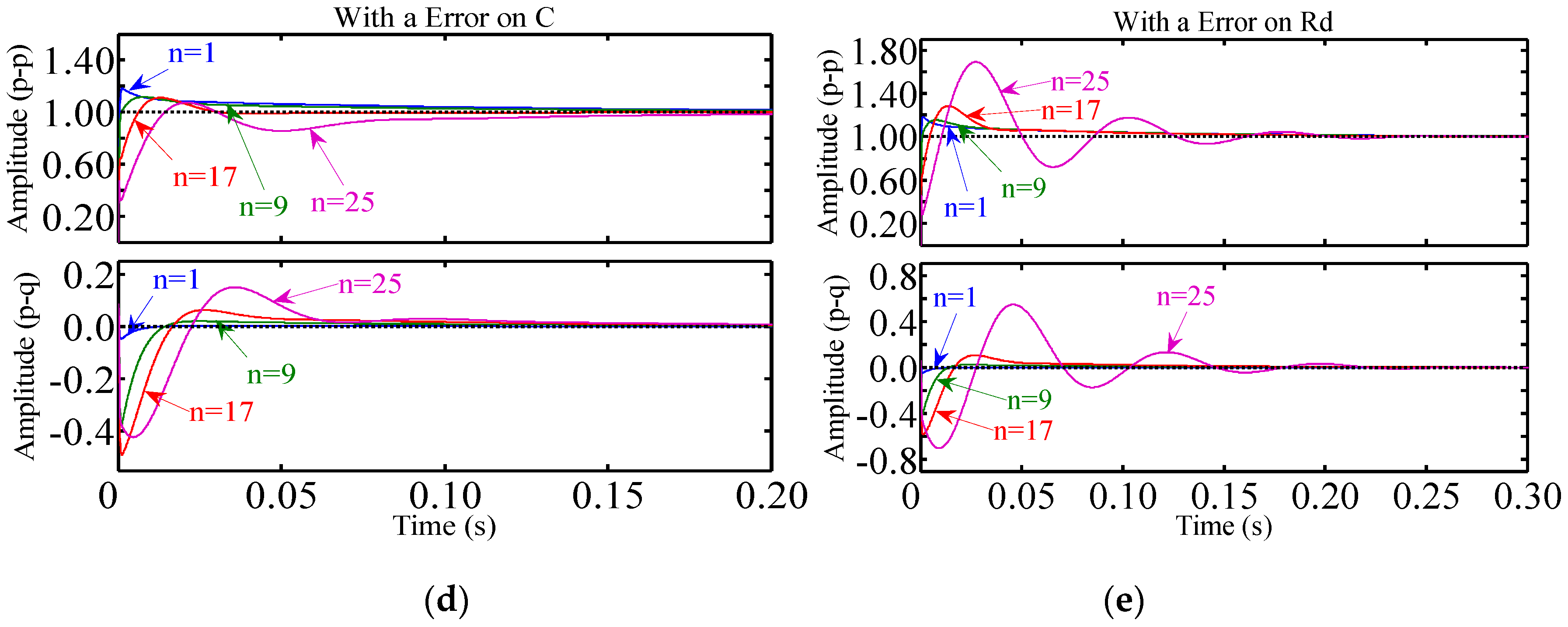
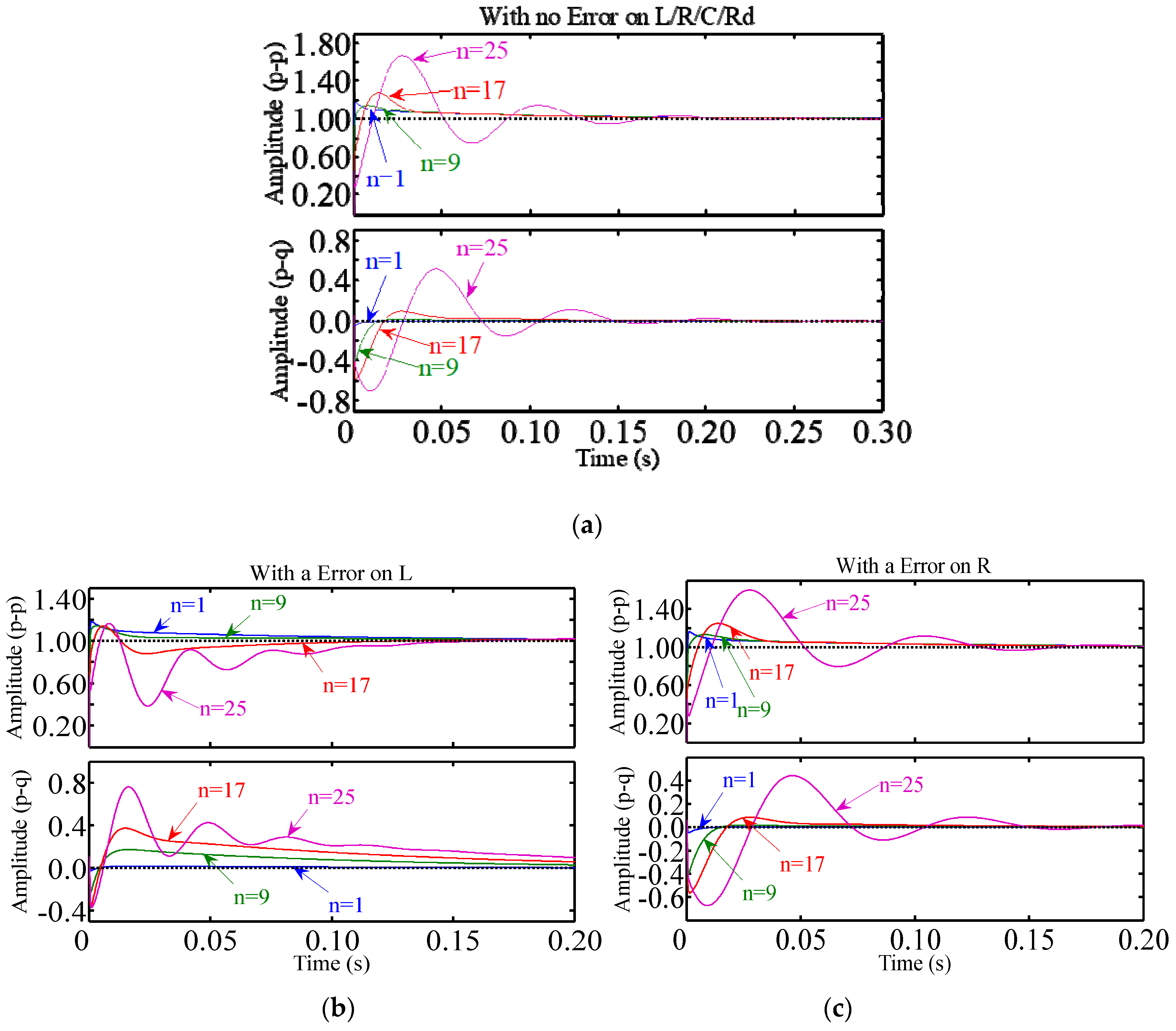
3.3. Performance Analysis for the Propsoed PBC Controller

Unit step responses of the modified control system are shown in Figure 5. Let the parameters L ≠ L_E, R ≠ R_E, C ≠ C_E and R_d ≠ R_dE, where the variation ranges of these parameters are both ± 50%, and the simulation parameters are as shown in

Table 1. Simulation parameters.

Parameter	Value	Parameter	Value	Parameter	Value
R	0.1 Ω	LE	0.9 mH	Ω	100 πrad/s
L	0.9 mH	RdE	200 Ω	rd	0.2
Rd	200 Ω	CE	10.0 uF	Ti	0.02 s
C	10.0 uF	Tω	0.02 s
RE	0.1 Ω	Ts	100 us

. The frequencies n = 1, 9, 17, and 25 are selected to simulate the system under on-load condition when parameters drift. It can be seen from Figure 5 that, although L ≠ L_E, R ≠ R_E, C ≠ C_E and R_d ≠ R_dE, the unit step responses of the forward channel of the modified control system equals are equal to 1 in the steady-state, the unit step responses of the coupled channel are equal to 0 in the steady-state, and the satisfied dynamic performance also can be obtained.

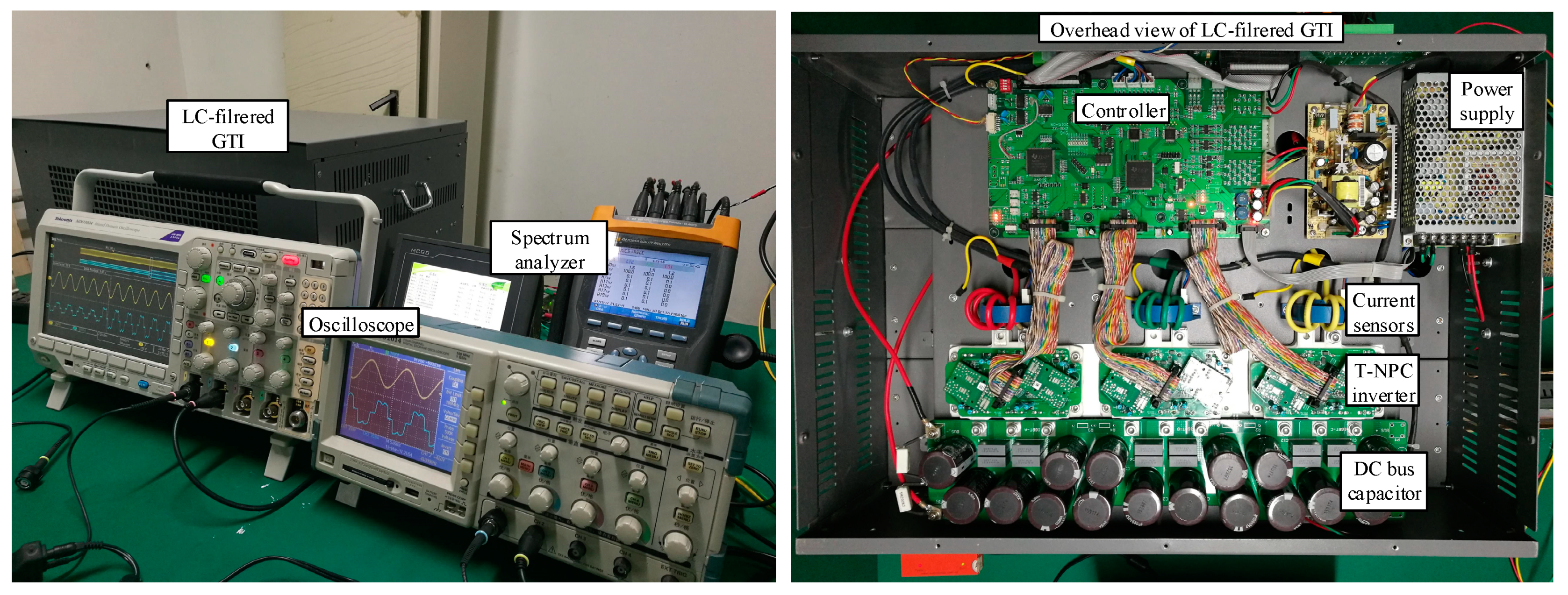
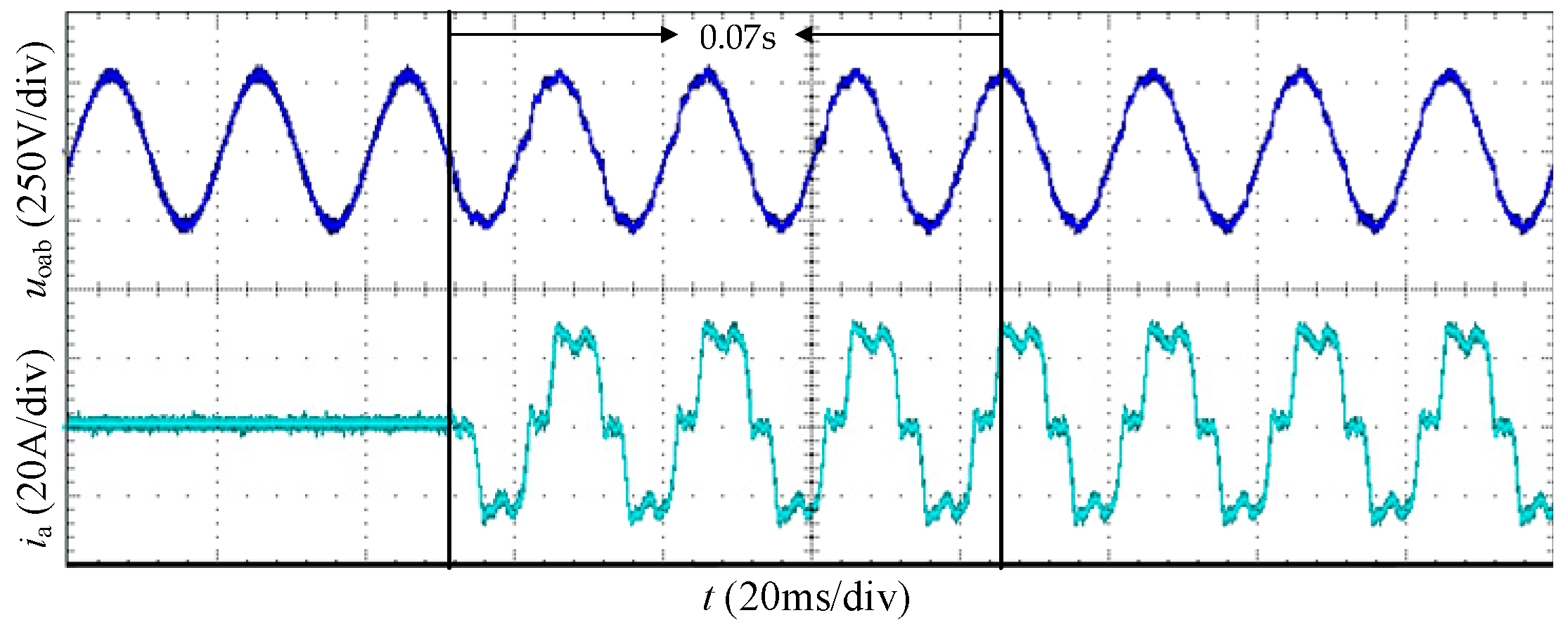
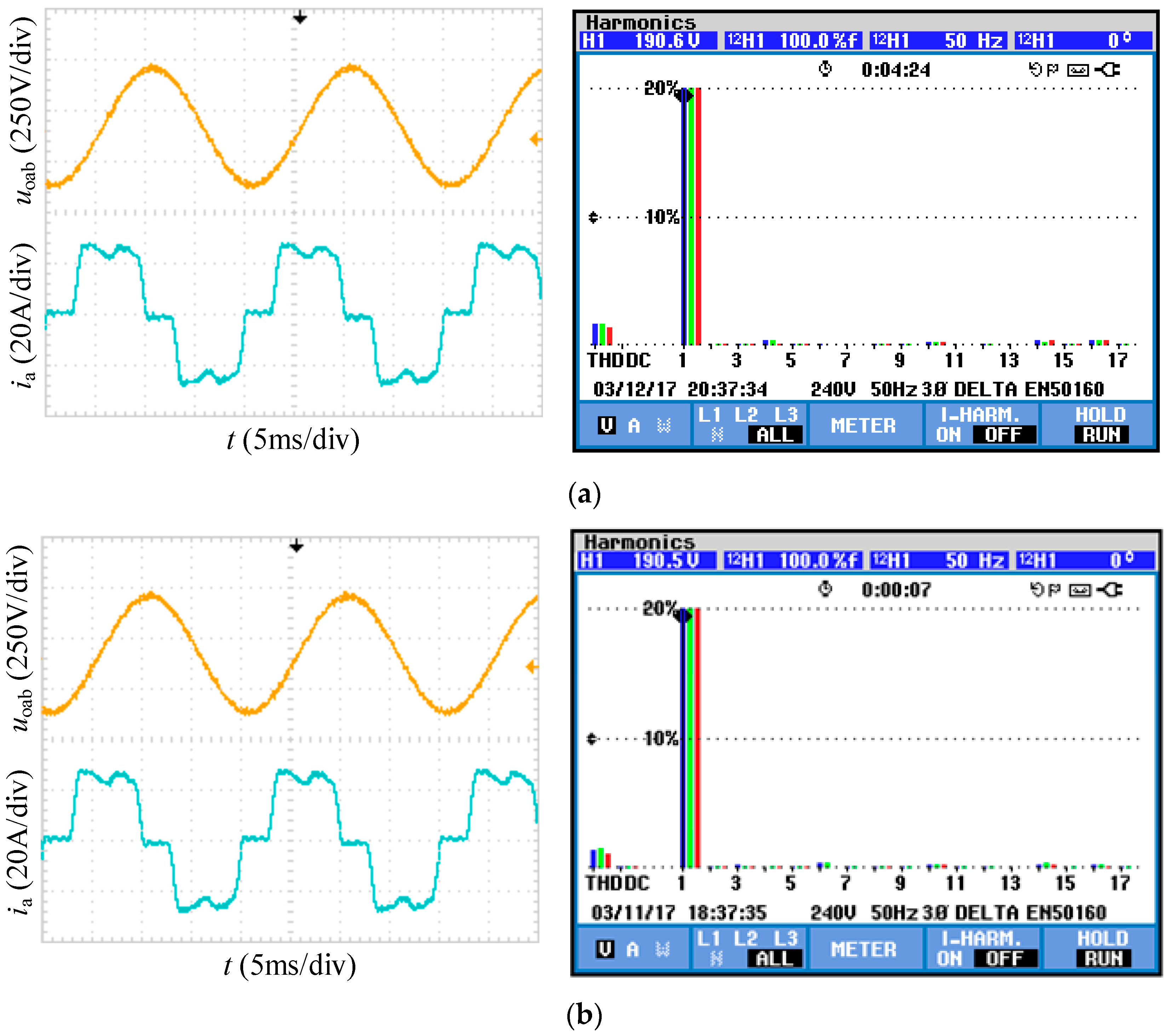
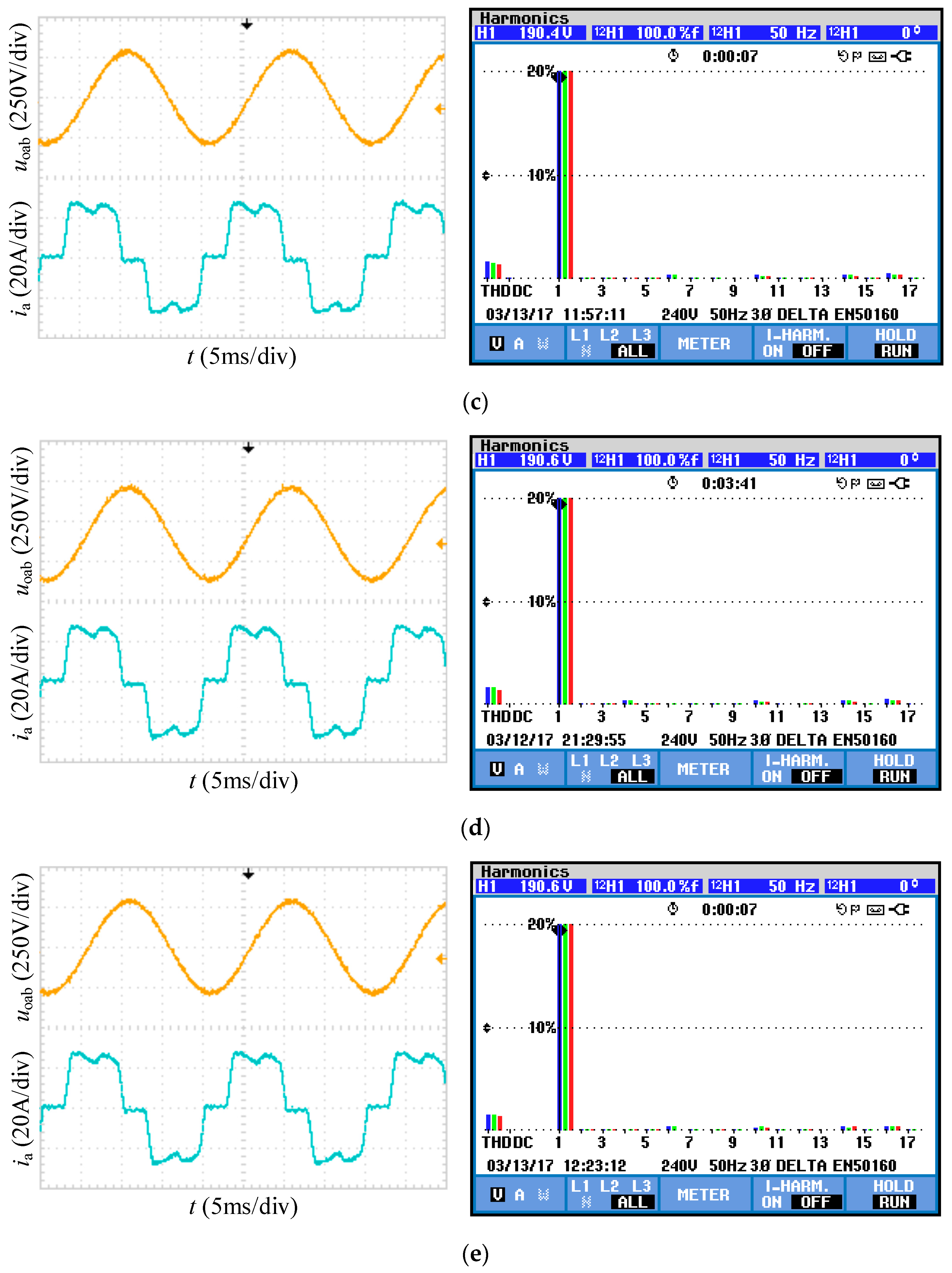
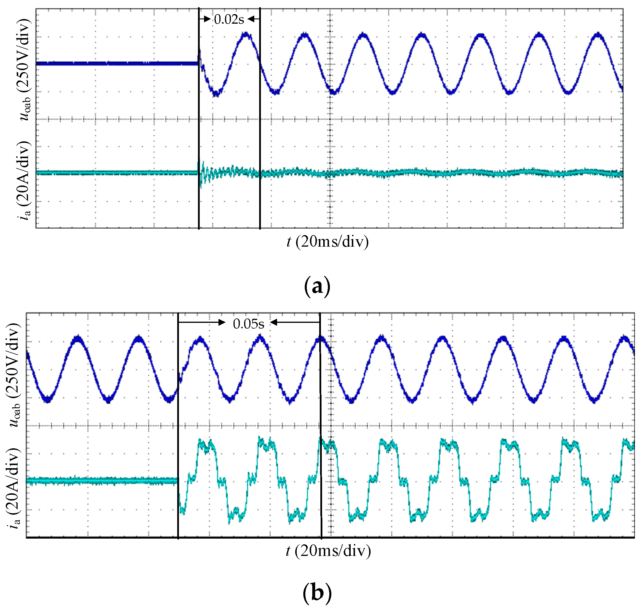
4. Experimental Verification

The whole converter structure shown in Figure 1 is adopted for the experimental platform. The nonlinear load current is realized by using a three-phase uncontrolled rectifier bridge with a resistor (11 Ω) and inductor (0.5 mH) load. The overall control scheme is shown in Figure 6, where the fundamental frequency peak reference voltage u_kp^1* = 110.0√2 V and u_kq^1* = 0.0 V; harmonic frequency peak command voltage u_kp^n* = 0.0 V and u_kq^n* = 0.0 V; and the DC link capacitor voltage u_dc = u_dc1 + u_dc2 = 400.0 V with C₁ = C₂ = 5.44 mF. Processor TMS320F28335DSP is used and the sampling and switching frequency are both 7.5 kHz. The execution time of the main programs is shown in

Table 2. The execution time of the main programs.

Procedural Content	Execution Time
Sampling period	133.33 us
Control algorithm at every selected frequency	16 us
ADC	8 us
Protection and communication	8 us

and the experimental setup is shown in Figure 7. Note that, the execution time of control algorithm at every selected frequency of the proposed PBC is 16 us, while it is 20 us in the conventional PBC (not shown in Table 2). Therefore, about 25 percent of time reduction is obtained.

As the nonlinear load used in the experiment mainly produces 6 m ± 1 order harmonic currents, where m = 1, 2, 3,…, its influence on the voltage is also concentrated at these harmonic frequencies. However, the harmonic current after the 19th order is already low, so its influence on the voltage formation at the point of common coupling (PCC) is weak. Therefore, in this experiment, the fundamental frequency and the 5th, 7th, 11th, 13th, 17th, and 19th frequencies are selected as the main control object for the experimental verification of the proposed multi-frequency single loop passivity-based control scheme.

Experiments are carried out to verify whether the reference voltage tracking (the fundamental wave voltage output and the harmonic voltage suppression) can be achieved, especially when the accurate mathematical model of the control object cannot be obtained. The experiments include five cases as following,

Case (1) Set the default estimation values L_E, R_E, C_E, and R_dE in the controller to the nominal values (L, R, C, and R_d) of the actual device, namely, let L_E = L= 0.9 mH, R_E = R = 0.1 Ω, C_E = C = 10 uF, and R_dE = R_d = 200 Ω; Case (2) Reduce L_E artificially by 50% to let L_E = 0.45 mH ≠ L, and keep other model parameters unchanged; Case (3) Increase R_E artificially by 50% to let R_E = 0.15 Ω ≠ R, and keep other model parameters unchanged; Case (4) Reduce C_E artificially by 50% to let C_E = 5.0 uF ≠ C, and keep other model parameters unchanged; Case (5) Increase R_dE artificially by 50% to let R_dE = 300 Ω ≠ R_d, and keep other model parameters unchanged.

The results of the five-group experimental data are shown in Figure 8a–e. Each group of figures contains the filter capacitor line voltage and load current waveforms, as well as the histogram of the corresponding harmonic voltage content at 6 m ± 1 order.

The experimental data are organized in

Table 3. Experimental results from Figure 7.

Group	THD	uoab1	5th	7th	11th	13th	17th	19th
Ref.	\	190.5	0.0	0.0	0.0	0.0	0.0	0.0
1-MPBC	1.6	190.6	0.1	0.1	0.1	0.1	0.1	0.1
2-MPBC	1.5	190.5	0.1	0.1	0.1	0.1	0.1	0.1
3-MPBC	1.6	190.4	0.1	0.1	0.1	0.1	0.1	0.1
4-MPBC	1.6	190.6	0.1	0.1	0.1	0.1	0.2	0.2
5-MPBC	1.6	190.6	0.1	0.1	0.1	0.1	0.1	0.1

. The phase-ab line voltage u_oab of filter capacitor is taken as an example for analysis. THD represents the total harmonic distortion rate of u_oab, u_oab1 represents the fundamental frequency content of u_oab which can be obtained from the histogram, and n^t represents the percentage of each harmonic content to the fundamental frequency content.

As seen from Table 3, the line voltage fundamental values of the five-group experiments are between 190.4 V and 190.6 V, and the error among the command values is between −0.05% and +0.05%, the maximum THD is ≤1.6%, the maximum percentage of other selected harmonics content is ≤0.2%.

It can be concluded that, the modified multi-frequency single loop PBC controller can track the command signal accurately at selected frequencies with less sensors.

Besides, the second group of experimental parameters are used to verify the dynamic performance of the modified multi-frequency single loop PBC controller (because the change in inductance exerts the greatest impact on the system). The step dynamic response of the voltage command under no-load condition is shown in Figure 9a, and the current disturbance under the condition of step load changes is shown in Figure 9b. And the dynamic response using conventional PI control is shown in Figure 10. It can be seen that the modified multi-frequency single loop PBC controller has satisfactory dynamic performance under both no-load (where the regulation time is 0.02 s) and on-load (where the regulation time is 0.05 s) conditions, and the response time is faster than conventional PI control (where the regulation time is 0.07 s).

5. Conclusions

In this paper, a multi-frequency single-loop passivity-based control strategy is proposed in the frequency domain for the LC-filtered stand-alone VSI, where the FFT transformation and dynamic dissipation term are adopted to achieve the frequency spectral decomposition and zero steady-state error. The advantages of the proposed control strategy include:

(1)

Less control variables, less hardware and software resources are occupied, thereby the calculation time can be saved a lot.

(2)

Zero steady-state error can be obtained by using the dynamic dissipation term, while a satisfactory dynamic performance can be gotten under both no-load and on-load conditions.

The experimental results on a 3-phase/110 V/6 kW prototype has verified the proposed control scheme, which making it efficient to extend the multi-frequency passivity-based control to engineering practice, even for higher-order systems.

References

1. Wu, W.; He, Y.; Blaabjerg, F. An LLCL Power Filter for Single-Phase Grid-Tied Inverter. IEEE Trans. Power Electron. 2012, 27, 782–789. [Google Scholar] [CrossRef]
2. Aamir, M.; Mekhilef, S. An Online Transformerless Uninterruptible Power Supply (UPS) System with a Smaller Battery Bank for Low-Power Applications. IEEE Trans. Power Electron. 2017, 32, 233–247. [Google Scholar] [CrossRef]
3. Pichan, M.; Rastegar, H. Sliding-Mode Control of Four-Leg Inverter with Fixed Switching Frequency for Uninterruptible Power. IEEE Trans. Ind. Electron. 2017, 64, 6805–6814. [Google Scholar] [CrossRef]
4. Tamyurek, B. A High-Performance SPWM Controller for Three-Phase UPS Systems Operating Under Highly Nonlinear Loads. IEEE Trans. Power Electron. 2013, 28, 3689–3701. [Google Scholar] [CrossRef]
5. Michal, V. Three-Level PWM Floating H-Bridge Sinewave Power Inverter for High-Voltage and High-Efficiency Applications. IEEE Trans. Power Electron. 2016, 31, 4065–4074. [Google Scholar] [CrossRef]
6. Zheng, L.; Jiang, F.; Song, J.; Gao, Y.; Tian, M. A Discrete Time Repetitive Sliding Mode Control for Voltage Source Inverters. IEEE J. Emerg. Sel. Top. Power Electron. 2018, 6, 1553–1566. [Google Scholar] [CrossRef]
7. Zhang, Z.; Wu, W.; Shuai, Z.; Wang, X.; Luo, A.; Chung, H.S.H.; Blaabjerg, F. Principle and Robust Impedance-Based Design of Grid-tied Inverter with LLCL-Filter under Wide Variation of Grid-Reactance. IEEE Trans. Power Electron. 2019, 34, 4362–4374. [Google Scholar] [CrossRef]
8. Zou, Z.; Zhou, K.; Wang, Z.; Cheng, M. Fractional-order repetitive control of programmable ac power sources. IET Power Electron. 2014, 7, 431–438. [Google Scholar] [CrossRef]
9. Liu, T.; Wang, D.; Zhou, K. High-Performance Grid Simulator Using Parallel Structure Fractional Repetitive Control Parallel. IEEE Trans. Power Electron. 2016, 31, 2669–2679. [Google Scholar] [CrossRef]
10. Wang, D.; Tian, J.; Mao, C.; Lu, J.; Duan, Y.; Qiu, J.; Cai, H. A 10kV_400V_500kVA Electronic Power Transformer. IEEE Trans. Ind. Electron. 2016, 63, 6653–6663. [Google Scholar] [CrossRef]
11. She, X.; Huang, A.Q.; Burgos, R. Review of solid-state transformer technologies and their application in power distribution systems. IEEE J. Emerg. Sel. Top. Power Electron. 2013, 1, 186–198. [Google Scholar] [CrossRef]
12. Pichan, M.; Rastegar, H.; Monfared, M. Deadbeat Control of the Stand-Alone Four-Leg Inverter Considering the Effect of the Neutral Line Inductor. IEEE Trans. Ind. Electron. 2017, 64, 2592–2601. [Google Scholar] [CrossRef]
13. Lidozzi, A.; Ji, C.; Solero, L.; Zanchetta, P.; Crescimbini, F. Digital Deadbeat and Repetitive Combined Control for a Stand-Alone Four-Leg VSI. IEEE Trans. Ind. Appl. 2017, 53, 5624–5633. [Google Scholar] [CrossRef]
14. Liu, T.; Wang, D. Parallel Structure Fractional Repetitive Control for PWM Inverters. IEEE Trans. Ind. Electron. 2015, 62, 5045–5054. [Google Scholar] [CrossRef]
15. Lidozzi, A.; Solero, L.; Bifaretti, S.; Crescimbini, F. Sinusoidal voltage shaping of inverter-equipped stand-alone generating units. IEEE Trans. Ind. Electron. 2015, 62, 3557–3568. [Google Scholar] [CrossRef]
16. Wu, W.; Liu, Y.; He, Y.; Chung, H.S.H.; Liserre, M.; Blaabjerg, F. Damping methods for resonances caused by LCL-filter-based current-controlled grid-tied power inverters: An Overview. IEEE Trans. Ind. Electron. 2017, 64, 7402–7413. [Google Scholar] [CrossRef]
17. Lidozzi, A.; Di Benedetto, M.; Bifaretti, S.; Solero, L.; Crescimbini, F. Resonant controllers with three degrees of freedom for AC power electronic converters. IEEE Trans. Ind. Appl. 2015, 51, 4595–4604. [Google Scholar] [CrossRef]
18. Liu, Y.; Wu, W.; He, Y.; Lin, Z.; Blaabjerg, F.; Chung, H.S.H. An efficient and robust hybrid damper for LCL- or LLCL-based grid-tied inverter with strong grid-side harmonic voltage effect rejection. IEEE Trans. Ind. Electron. 2016, 63, 926–936. [Google Scholar] [CrossRef]
19. Sebaaly, F.; Vahedi, H.; Kanaan, H.Y.; Moubayed, N.; Al-Haddad, K. Sliding Mode Fixed Frequency Current Controller Design for Grid-Connected NPC Inverter. IEEE J. Emerg. Sel. Top. Power Electron. 2016, 4, 1397–1405. [Google Scholar] [CrossRef]
20. Gudey, S.K.; Gupta, R. Reduced state feedback sliding-mode current control for voltage source inverter-based higher-order circuit. IET Power Electron. 2015, 8, 1367–1376. [Google Scholar] [CrossRef]
21. Wang, L.; Lam, C.S.; Wong, M.C.; Dai, N.Y.; Lao, K.W.; Wong, C.K. Non-linear adaptive hysteresis band pulse-width modulation control for hybrid active power filters to reduce switching loss. IET Power Electron. 2015, 8, 2156–2167. [Google Scholar] [CrossRef]
22. Yaramasu, V.; Rivera, M.; Narimani, M.; Wu, B.; Rodriguez, J. Model Predictive Approach for a Simple and Effective Load Voltage Control of Four-Leg Inverter with an Output LC Filter. IEEE Trans. Ind. Electron. 2014, 61, 5259–5270. [Google Scholar] [CrossRef]
23. Rohten, J.A.; Espinoza, J.R.; Muñoz, J.A.; Pérez, M.A.; Melin, P.E.; Silva, J.J.; Rivera, M.E. Model Predictive Control for Power Converters in a Distorted Three-Phase Power Supply. IEEE Trans. Ind. Electron. 2016, 63, 5838–5848. [Google Scholar] [CrossRef]
24. Do, T.D.; Leu, V.Q.; Choi, Y.S.; Choi, H.H.; Jung, J.W. An adaptive voltage control strategy of three-phase inverter for stand-alone distributed generation systems. IEEE Trans. Ind. Electron. 2013, 60, 5660–5672. [Google Scholar] [CrossRef]
25. Kim, E.K.; Mwasilu, F.; Choi, H.H.; Jung, J.W. An Observer-Based Optimal Voltage Control Scheme for Three-Phase UPS Systems. IEEE Trans. Ind. Electron. 2015, 62, 2073–2081. [Google Scholar] [CrossRef]
26. Komurcugil, H. Improved passivity-based control method and its robustness analysis for single-phase uninterruptible power supply inverters. IET Power Electron. 2015, 8, 1558–1570. [Google Scholar] [CrossRef]
27. Ortega, R.; Perez, J.A.L.; Nicklasson, P.J.; Sira-Ramirez, H.J. Passivity-Based Control of Euler-Lagrange Systems: Mechanical Electrical and Electromechanical Application; Springer: London, UK, 1998. [Google Scholar]
28. Lee, T.S. Lagrangian modeling and passivity-based control of three phase AC/DC voltage-source converters. IEEE Trans. Ind. Electron. 2004, 51, 892–902. [Google Scholar] [CrossRef]
29. Mehrasa, M.; Adabi, M.E.; Pouresmaeil, E.; Adabi, J. Passivity-based control technique for integration of DG resources into the power grid. Int. J. Electr. Power Energy Syst. 2014, 58, 281–290. [Google Scholar] [CrossRef]
30. Yang, B.; Jiang, L.; Yu, T.; Shu, H.C.; Zhang, C.K.; Yao, W.; Wu, Q.H. Passive control design for multi-terminal VSC-HVDC systems via energy shaping. Int. J. Electr. Power Energy Syst. 2018, 98, 496–508. [Google Scholar] [CrossRef]
31. Xu, R.; Yu, Y.; Yang, R.; Wang, G.; Xu, D.; Li, B.; Sui, S. A Novel Control Method for Transformerless H-Bridge Cascaded STATCOM with Star Configuration. IEEE Trans. Power Electron. 2015, 30, 1189–1202. [Google Scholar] [CrossRef]
32. Chen, Y.; Wen, M.; Lei, E.; Yin, X.; Lai, J.; Wang, Z. Passivity-based control of cascaded multilevel converter based D-STATCOM integrated with distribution transformer. Electr. Power Syst. Res. 2018, 154, 1–12. [Google Scholar] [CrossRef]
33. Del Puerto-Flores, D.; Scherpen, J.M.; Liserre, M.; de Vries, M.M.; Kransse, M.J.; Monopoli, V.G. Passivity-based control by series/parallel damping of single-phase PWM voltage source converter. IEEE Trans. Control Syst. Technol. 2014, 22, 1310–1322. [Google Scholar] [CrossRef] [Green Version]
34. Gui, Y.; Kim, W.; Chung, C.C. Passivity-based control with nonlinear damping for type 2 STATCOM systems. IEEE Trans. Power Syst. 2016, 31, 2824–2833. [Google Scholar] [CrossRef]
35. Serra, F.M.; Angelo, C.H.D.; Forchetti, D.G. Interconnection and damping assignment control of a three-phase front end converter. Int. J. Electr. Power Energy Syst. 2014, 60, 317–324. [Google Scholar] [CrossRef]
36. Fan, X.; Guan, L.; Xia, C.; Ji, T. IDA-PB control design for VSC-HVDC transmission based on PCHD model. Int. Trans. Electr. Energy Syst. 2015, 25, 2133–2143. [Google Scholar] [CrossRef]
37. Tiantian, Q.; Shihong, M.; Ziwen, L. Passive Control and Auxiliary Sliding Mode Control Strategy for VSC-HVDC System Based on PCHD Model. Trans. China Electrotech. Soc. 2016, 31, 138–144. [Google Scholar]
38. Mu, X.; Wang, J.; Wu, W.; Blaabjerg, F. A Modified Multifrequency Passivity-Based Control for Shunt Active Power Filter with Model-Parameter-Adaptive Capability. IEEE Trans. Ind. Electron. 2018, 65, 760–769. [Google Scholar] [CrossRef]
39. Wang, J.; Mu, X.; Li, Q. Study of Passivity-Based Decoupling Control of T-NPC PV Grid-Connected Inverter. IEEE Trans. Ind. Electron. 2017, 64, 7542–7551. [Google Scholar] [CrossRef]
40. Akagi, H.; Kanazawa, Y.; Nabae, A. Instantaneous reactive power compensators comprising switching devices without energy storage components. IEEE Trans. Ind. Appl. 1984, IA-20, 625–630. [Google Scholar] [CrossRef]
Figure 1. Typical structure of the stand-alone Voltage Source Inverter(VSI).
Energies 12 04548 g001
Figure 2. Single Alternating Current to Direct current (AC-to-DC) model transformation using FFT. (a) single phase ac model, (b) single phase dc model.
Energies 12 04548 g002aEnergies 12 04548 g002b
Figure 3. Conventional Passivity-Based Control (C-PBC) control structure.
Energies 12 04548 g003
Figure 4. Modified multi-frequency single loop PBC control scheme.
Energies 12 04548 g004
Figure 5. Unit step response of the modified control under different situations.
Energies 12 04548 g005aEnergies 12 04548 g005b
Figure 6. Overall control scheme.
Energies 12 04548 g006
Figure 7. Experimental setup.
Energies 12 04548 g007
Figure 8. Experimental data using multi-frequency single loop PBC controller under different situation, (a) Case (1), (b) Case (2), (c) Case (3), (d) Case (4), (e) Case (5).
Energies 12 04548 g008aEnergies 12 04548 g008b
Figure 9. Dynamic response of the improved multi-frequency cascade passivity-based control, (a) under no-load situation, (b) under on-load situation.
Energies 12 04548 g009
Figure 10. Dynamic response of the Proportional Integral (PI) control.
Energies 12 04548 g010