Convection Heat Transfer Coefficients in Thermoacoustic Heat Exchangers: An Experimental Investigation

Abstract

This paper investigates the thermal performance of thermoacoustic heat exchangers subjected to acoustically oscillating flows. The analysis is carried out by experimental measurements of the heat fluxes sustained by the ambient heat exchanger of a prime mover of the standing wave type. A home-made parallel-plate heat exchanger is considered for the study. The gas-side convection heat transfer coefficients expressed as Nusselt numbers are determined over a wide range of velocity amplitudes of the oscillating flow. The experimental results are then compared to the predictions of a number of theoretical models currently applied in thermoacoustics such as the time-average steady-flow equivalent (TASFE) model, the root mean square Reynolds number (RMS-Re) model, and the boundary layer conduction model. The comparison suggests that the boundary layer model performs better than the rms-Re and TASFE models in predicting the heat transfer coefficients in oscillating flows. The relative difference between the model predictions and the experimental data amounts to 19%. A new correlation law, based on regression of the experimental data, is also proposed.

1. Introduction

Thermoacoustic (TA) engines are energy conversion devices whose operation relies on the cyclic heat transfer experienced by an acoustically oscillating gas with the solid walls of a porous medium. This technology, including prime movers, refrigerators, and heat pumps, has recently received increasing attention for having high potential to be a reliable, low-cost, and environmentally friendly technology, with remarkable applications in the renewable energy and waste heat recovery sectors.

Although the theoretical basis of TA systems is well established (the so-called linear theory of thermoacoustics [1,2,3,4]), the behavior of some components has not yet received proper mathematical modelling. The major of these components is the heat exchanger (HX) for which well-established design methodologies are still not available. This lack of knowledge derives from the TA HXs being subjected to oscillatory flows. This means that the fluid particles periodically reverse their direction of flow over a distance equal to the peak-to-peak particle displacement amplitude. Therefore, an arbitrary increase in the HX length could not automatically lead to an increase of the heat transfer area but, eventually, only to an increase of the thermoviscous dissipation [4]. Therefore, when designing efficient HXs, the HX length must be simultaneously optimized with the pore hydraulic diameter and the fin thickness (or, equivalently, the HX blockage ratio) in order for the target heat load to be transferred under a small gas-solid temperature difference in conjunction with low pressure drop [5,6].

This type of calculation, however, requires the knowledge of the gas-side heat transfer coefficient as a necessary prerequisite, which, due to the oscillatory character of the flow, cannot be derived from conventional correlation laws for compact HXs generally referring to steady fluid flows.

There are only a few studies in the literature concerned with the experimental determination of heat transfer correlations for oscillatory flows and that could serve as a basis for theoretical modelling.

Paek et al. [7] carried out an experimental investigation of the thermal performance of a parallel-plate HX acting as the cold HX of a TA cooler. A heat transfer correlation in terms of Colburn-j factor was proposed.

Thermoacoustic coolers were also used by Nsofor et al. [8] and Tang et al. [9] to investigate the gas side heat transfer coefficient of HXs of the parallel-plate type.

Experiments involving standing wave devices with two identical HXs and no stack in between were conducted by Kamsanam et al. [10] and Ilori et al. [11] to investigate the thermal performance of HXs of the parallel-plate type and parallel tube type. The derived correlation laws were expressed in terms of Nusselt numbers.

All the above studies indicate that steady flow heat transfer correlations for compact HXs could be not applicable for TA applications, since they may introduce significant errors in predicting the gas-side convection coefficient. Deviations between experimental data and model predictions as high as 71.3% were found in [10], although Paek et al. [7] found deviations of about 38% that further decreased by making improvements in the correlation model. As for the “boundary layer heat transfer model”, currently integrated in DeltaEC [12] (the main simulation code of TA devices), deviations as high as 114% were found in [7] and as low as 21.5% were found in [9]. The results reported in these studies are therefore not univocal and need further validation. Therefore, additional experimental investigations could be useful to expand the range of operative conditions and geometrical configurations.

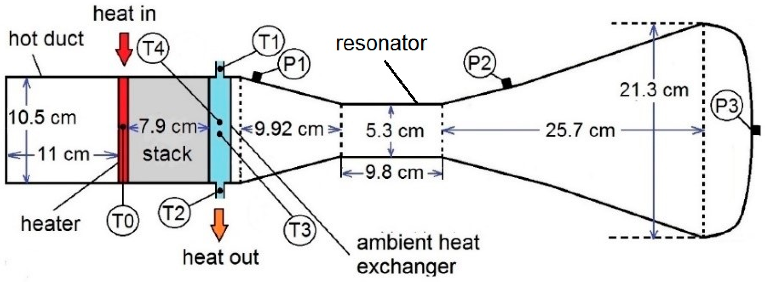
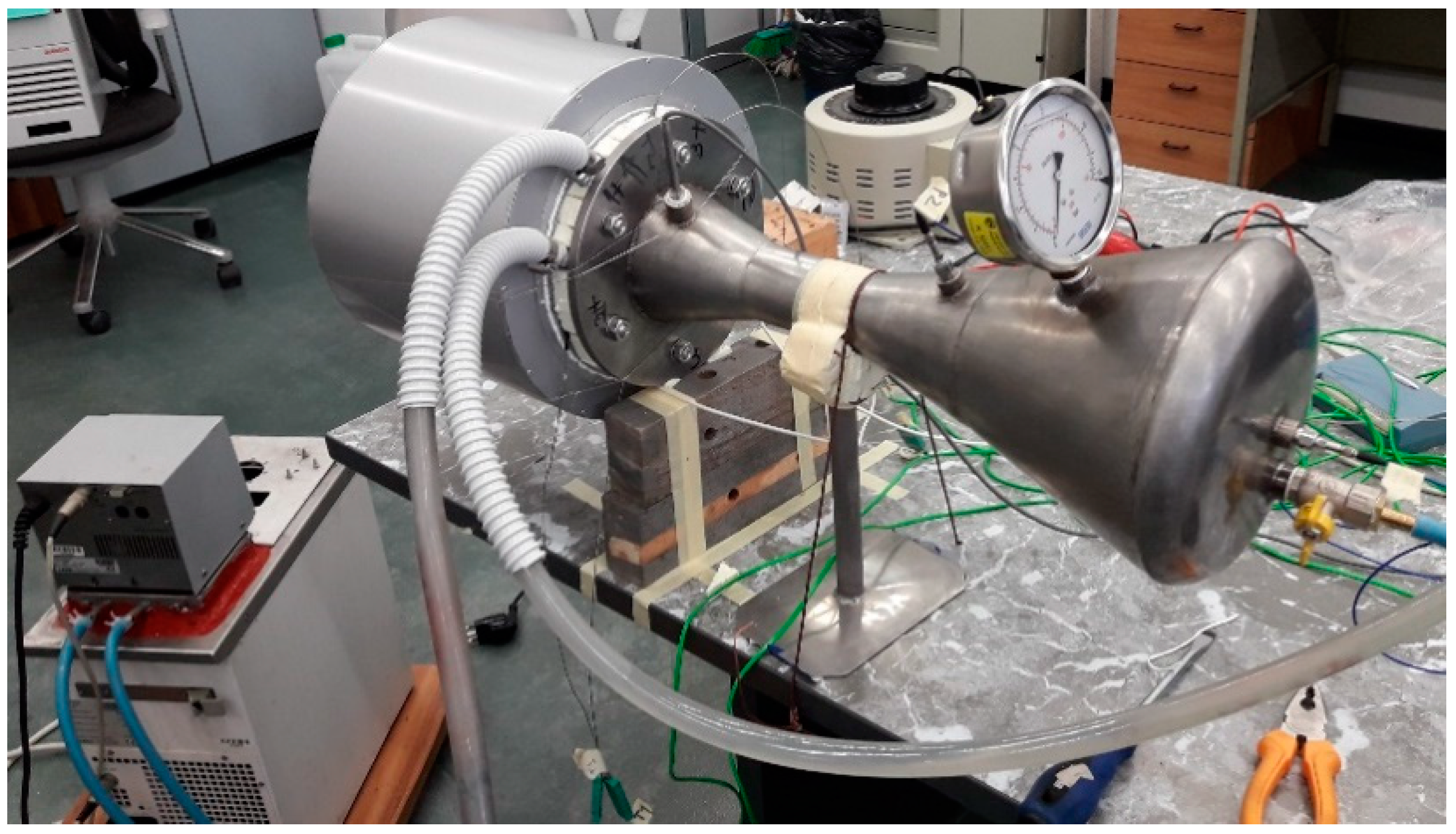
With this aim, in this paper, an experimental study of the thermal performance of a TA HX is carried out. The work involves the determination of the heat fluxes sustained by a HX of the finned-tube type through standard heat balance measurements. This HX functions as an ambient HX of a prime mover of the standing wave type, a configuration not considered in the above cited investigations and that needs a specific data reduction. From the experimental data, the gas-side heat transfer coefficient over a wide range of velocity amplitudes is calculated. A new correlation law expressed in terms of dimensionless Nusselt number is then derived and compared to a number of theoretical models currently applied in thermoacoustics. This new proposed correlation could be usefully applied in the design of practical TA HXs.

2. Experimental Setup

The experimental apparatus used in the present study is entirely homemade and consists of a thermoacoustic engine of the standing-wave type working with air at atmospheric pressure. A schematic of the engine is shown in Figure 1. The engine comprises an acoustic resonator (acting as a pressure vessel and fixing the resonance frequency), a stack (converting heat to acoustic power), an electric heater (supplying the driving heat to the system), and an ambient HX (extracting a fraction of the input heat from the engine). The engine starts to oscillate when the temperature difference between the hot and ambient edges of the stack overcomes an onset value (~350 °C for the experimental conditions of the present study). The measured resonance frequency is 143.2 Hz when the engine is driven by a heat input of 150 W.

2.1. Resonator

The resonator is a stainless-steel duct with a variable cross section profile for inhibiting the harmonic generation phenomenon [13,14] and for allowing one to match the design operation frequency (~143 Hz) by a total length shorter than the one required by a straight resonator. It serves to define the working frequency of the engine and to force the stack to work under an acoustic field typical of a standing wave (pressure-velocity phase angle ≈90°). The resonator is made up of a “hot” duct with a diameter of 10.5 and a length of 10 cm, a stack holder with a diameter of 10.5 cm and a length of 8 cm long, a conical-shaped duct with a length of 7.8 cm and reducing the diameter from 10.5 cm to 5.3 cm, a narrow duct with a diameter of 5.3 cm and a length of 20 cm, and a closed conical-shaped duct acting as a buffer volume. A pressure microphone (Brüel and Kjær instruments, type 4938, sensitivity 1.6 mV/Pa) and two piezoelectric pressure transducers (PCB Piezotronics, model 113B28, sensitivity 14.5 mV/kPa) are flush mounted on the resonator walls. They are indicated with labels P1, P2, and P3 in Figure 1.

2.2. Stack

The stack holder accommodates a ceramic honeycomb stack with a low thermal conductivity and a high specific heat, as required to improve the heat to acoustic power energy conversion efficiency [1]. This stack is characterized by a cell density near 400 cells per square inch (cpsi) and has pores of squared shape with a hydraulic radius of around 0.28 mm. A picture of the stack is shown in Figure 2.

2.3. Heater

The electric heater, placed between the “hot” duct and the stack holder, is made up of a 1-cm-long ceramic honeycomb slice. About 3.7 m of a Ni-Cr wire (12 Ω/m) are passed uniformly through its pores. The slice is fitted in one side of a 2-cm-long stainless-steel ring equipped with feedthroughs for power cables. A Type K thermocouple (error ±0.3 °C), labeled as T0 in Figure 1, was placed in the central region of the ceramic matrix (inside a pore). Since the probe touched the wall of the pore, it presumably measured the average temperature (T_H) of the wall and oscillating gas. A picture of the heater is shown in Figure 3.

2.4. Heat Exchanger

The homemade ambient HX prototype is a 2-cm-long water-cooled HX of the crossflow type with four water-tube passes. A 2-cm-thick copper ring with an internal radius of 10.5 cm and an external radius of 14 cm was used as mechanical support for its manufacturing. The water tubes are obtained from a unique copper tube having an inside diameter of 14 mm and a wall thickness of 1 mm. By crushing it, a rectangular cross-section pipe of area 2 cm × 0.5 cm was obtained. This last part was then bent six times, allowing for four passages in the front section of the HX, as shown in Figure 4.

Fins made of laminated copper were welded to the external walls of the pipe by a brazing technique. The fin thickness and spacing are 0.45 mm and 1.1 mm, respectively while the HX blockage ratio (BR), i.e., the ratio of the open to the total cross-section area, is around 54%. Four thermocouples (Type K) are placed in this HX to measure the temperatures of interest. Two of these thermocouples (labeled as T1 and T2 in Figure 1) are installed in the water tubing just outside the HX to measure the inlet temperature (T₁) and the outlet temperature (T₂) of the cooling water. One thermocouple (labeled as T3) was suspended through a spacer in the (slightly enlarged) gap between two fins located in the central region of the HX. It measured the temperature of the gas oscillating inside a pore (T_g). The other thermocouple (labeled as T4) was glued through a copper spray to the wall of the crushed copper pipe just near the previous thermocouple. It measured the temperature T_s of the wall pipe, which the fins are welded to (i.e., the temperature at the base of the fins).

The length of the HX along the resonator axis was selected to be 2 cm since preliminary simulations performed by the DeltaEC code [12] indicated that this length is comparable, at the typical operative conditions of the present study, to the peak-to-peak particle oscillation amplitude. As for the HX pores, they were selected to have a hydraulic radius R_h = 0.5 mm. This should ensure a good thermal contact between the gas and the HX walls since the thermal penetration depth of the gas, i.e., the distance through which heat diffuses in an acoustic period

$${\delta }_{\kappa }=\sqrt{\frac{2\kappa }{\omega }},$$

(1)

(κ and ω are the gas thermal diffusivity and the angular frequency, respectively) amounts to δ_κ ≈ 0.22 mm at the resonance frequency of the engine (f ≈ 143 Hz) so that R_h/δ_κ ≈ 2 [15].

A picture of the standing wave engine in place for testing is shown in Figure 5. On the left, the cylindrical thermally insulating cap filled with rock wool used to minimize thermal leakage from the hot segments of the engine (“hot duct, electric heater, and stack holder) to the environment is visible.

3. Calculation Methodology

To estimate the heat transfer rates sustained by the ambient HX and the related gas-side heat transfer coefficient, a procedure based on standard energy balance calculations was applied. The heat flux transferred by the HX was estimated from the measured values of the inlet and outlet water temperatures and of the water volume flow rate, V_a, as

$$Q_A=V_a{\rho }_a{c}_a(T_2-T_1)$$

(2)

where c_a and ρ_a are the specific heat and density of water, respectively. This heat flux comprises the heat flux Q transported hydrodynamically by the acoustic wave along the stack, the heat flux Q_K1 transported by thermal conduction in the stack (both by the gas and the solid), the heat flux Q_K2 transported by thermal conduction by the stack-holder walls and thermal insulating sleeve, and the heat flux Q_K3 originating from dissipation of acoustic power and transported by thermal conduction in the resonator walls to the ambient HX where it is extracted. Therefore, to estimate Q (which enters in the calculation of the gas-side heat transfer coefficient), the conduction contribution Q_K = Q_K1 + Q_K2+ Q_K3 has to be subtracted from Q_A:

$$Q=Q_A-Q_K=Q-(Q_{K1}+Q_{K2}+Q_{K3}).$$

(3)

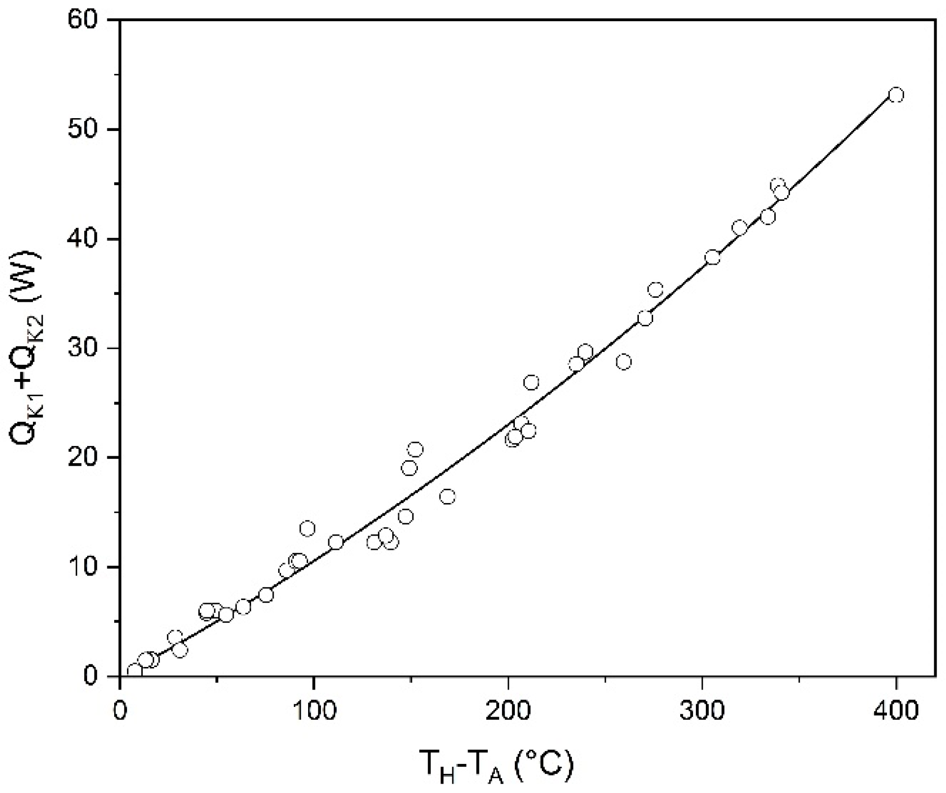
With this aim, the heat flux (Q_K1 + Q_K2) was experimentally determined once for all by powering the heater below the onset temperature of the engine and measuring the thermal load on the AHX. Results are shown in Figure 6 where (Q_K1 + Q_K2) is plotted against the temperature difference between the heater, T_H, and the ambient heat exchanger, T_A = (T_s + T_g)/2. As for the Q_K3 contribution, it was estimated by simulating the energy fluxes in the engine by the DeltaEC code where the experimental values recorded by the dynamic pressure sensors P1, P2, and P3 were used as inputs for model refinements. By this procedure, the Q values resulted about 25% lower than the measured Q_A values.

To make the calculated Q consistent with the inlet and outlet temperatures of water, the Q_K contribution to the inlet—outlet temperature difference was subtracted from the measured values of T₂ as follows

$$T_2^{\prime }=T_2-\frac{Q_K}{V_a{\rho }_a{c}_a}$$

(4)

where T₂′ is the outlet temperature of water that would be measured if the Q_K contribution was absent, i.e., if the HX was uniquely loaded by the convection heat flux. By this procedure, the T₂ values decreased by about 2.5%.

According to Paek et al. [7] and Kamsanam et al. [10], HXs found in thermoacoustic devices are typically of the crossflow type so the log-mean-temperature-difference (LMTD) method can be conveniently applied for the calculation of the heat transfer rates. In this method, the overall heat transfer coefficient, UA, is defined as

$$UA=\frac{Q}{{\theta }_{ml}}$$

(5)

where θ_ml, the log-mean temperature difference, is defined as

$${\theta }_{ml}=\frac{T_2^{\prime }-T_1}{\ln \left(\frac{T_g-T_1}{T_g-T_2^{\prime }}\right)}.$$

(6)

Note that in Equation (6), the inlet and outlet temperatures of the primary fluid (the gas) are the same (T_g), being the flow oscillatory. Once Q and θ_ml are calculated from the experimental data through Equations (2)–(4) and (6), they can be substituted in Equation (5) to determine the overall heat transfer coefficient UA. The estimation of the gas-side heat transfer coefficient is then done, considering that for the geometry of the investigated HX, UA has the following expression [16]:

$$UA=\frac{1}{\frac{1}{h_a{A}_i}+\frac{d}{K_t{A}_i}+\frac{1}{h\left[{\displaystyle \sum _i(\mathsf{\Pi }{L}_{fi}){\eta }_{fi}+A_b}\right]}}$$

(7)

where A_i, K_t, and d are the total inner surface, the thermal conductivity, and the wall thickness of the copper tube, respectively; h_a and h are the water-side and gas-side heat transfer coefficients, respectively; Π and L_fi are the cross section perimeter and half the length of the i-th fin, respectively; A_b is the total area of the un-finned surface of the tubes; and η_fi, the efficiency of the i-th fin, has the following expression

$${\eta }_{fi}=\frac{\tanh (m{L}_{fi})}{m{L}_{fi}}\hspace{1em}\hspace{1em}\hspace{1em}\left(m=\sqrt{\frac{h\mathsf{\Pi }}{A_f{K}_f}}\right).$$

(8)

K_f and A_f are the thermal conductivity and cross-section area and of the fin, respectively.

The application of Equation (7) requires preliminary the determination of the water-side heat transfer coefficient h_a. With this purpose, the HX was immersed in a water bath with temperature controlled at 50 °C by a refrigerator/heating circulator. This served to maintain the HX in isothermal conditions while a flow of water at 25 °C was sent to the inlet section of the HX. Taking into account that the temperature drop across the copper wall of the water tube is negligible (being that the wall is thin, d ≈ 1 mm, and of high thermal conductivity, K_t ≈ 400 W/mK), the measured temperature of the fin base T_s is assumed to be equal to the temperature of the internal surfaces of the water tube. Recalling now the energy balance equations for the case of internal flow with constant surface temperature [16], the measured values of T₁, T₂, and T_s allow one to estimate h_a through the equation

$$h_a=\frac{V_a{\rho }_a{c}_a}{A_i}\ln \left(\frac{T_s-T_1}{T_s-T_2}\right).$$

(9)

For a water flow rate of 60 l/h, for example, the method furnished the value h_a = 2495 ± 21 W/m²K (the indicated accuracy being the standard deviation of measurements).

The measurement uncertainty is estimated on the basis of standard formulas for error propagation [17]. To increase the accuracy in the measurement of temperature differences (ΔT), the thermocouples have been previously calibrated in situ by an environmental test chamber. This reduced the error in ΔT to ±0.2 °C. The accuracy in the measurement of the flow rate of water was 0.0048 L/min. The uncertainty on Nusselt number is estimated to be around 20%.

4. Results and Discussion

The heat transfer coefficients estimated as previously described and expressed in terms of dimensionless Nusselt numbers

$$\mathrm{Nu}=\frac{h{D}_h}{K}$$

(10)

(D_h being the hydraulic diameter of the HX pores and K the gas thermal conductivity) are correlated to the local peak acoustic Reynolds number

$${\mathrm{Re}}_1=\frac{{\rho }_0{D}_h{v}_1}{\eta },$$

(11)

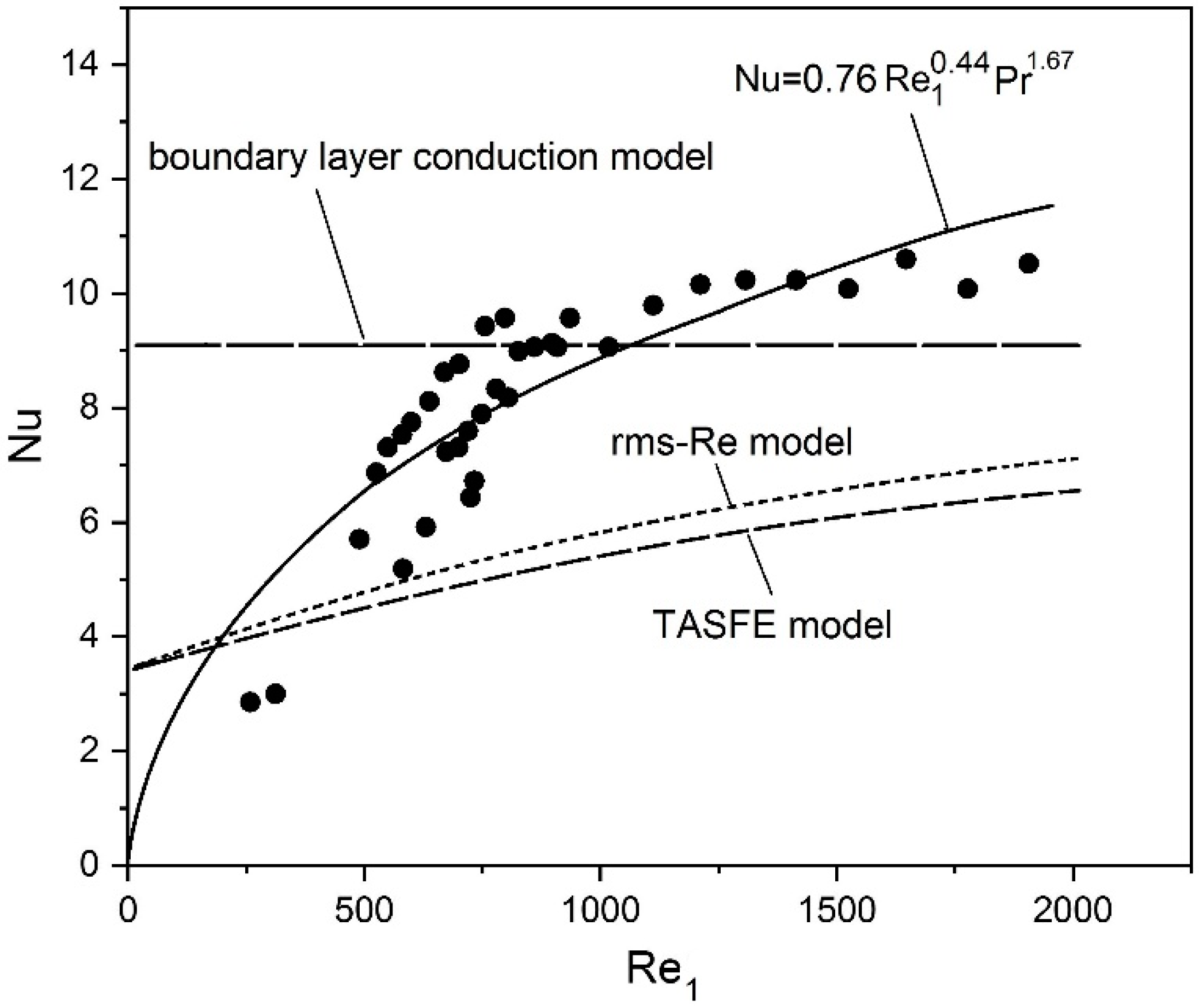
ρ₀ being the mean gas density, η the dynamic viscosity, and v₁ the acoustic velocity amplitude calculated by simulating the standing-wave engine by the DeltaEC code [12] (where the pressure values measured by P1, P2, and P3 were used for iterative refinements of the model). The experimental results are shown in Figure 7 (full circles) together with the regression curve (continuous line) obtained by fitting the data by the function

$$\mathrm{Nu}=a{\mathrm{Re}}^b{\mathrm{Pr}}^c$$

(12)

where the values obtained for parameters a, b, and c were 0.76, 0.44, and 1.67, respectively. Other correlation laws, derived by heat transfer models currently applied in thermoacoustics, are also shown.

The long dashed line refers to the “boundary layer conduction heat transfer” model proposed by Swift [3]. The model (implemented in DeltaEC) calculates the heat transfer coefficient h by the relation

$$h=\frac{K}{y_{eff}}$$

(13)

where y_eff = min {y₀, δ_κ}.

The short dashed line refers to the “time-average steady-flow equivalent” (TASFE) model [18]. This model derives proper heat transfer correlation laws for the oscillatory flow regime by taking the time average over an acoustic cycle of classical steady flow correlations for compact HX. The Hausen correlation [16] for laminar flow is considered in the present work:

$${\overline{\mathrm{Nu}}}_D=3.66+\frac{0.0668(D/L_T)\mathrm{Pr}{\mathrm{Re}}_D}{1+0.04{[(D/L_T)\mathrm{Pr}{\mathrm{Re}}_D]}^{2/3}},$$

(14)

D being the diameter of the duct, L_T the thermal entry length, and Re_D the Reynolds number. The TASFE correlation resulting from taking the time-average of Equation (14) over half the acoustic period is

$${\overline{\mathrm{Nu}}}_D=\frac{1}{\pi }{\displaystyle \underset{0}{\overset{\pi /\omega }{\int }}\left\{3.66+\frac{0.0668(D_h/L_{HX})\mathrm{Pr}{\mathrm{Re}}_{1,D}\sin \omega t}{1+0.04{[(D_h/L_{HX})\mathrm{Pr}{\mathrm{Re}}_{1,D}\sin \omega t]}^{2/3}}\right\}}\hspace{0.17em}dt.$$

(15)

The dotted line refers to the “root mean square Reynolds number” (rms-Re) [18]. In this model, the Reynolds numbers, figuring in conventional steady flow correlations, are substituted by their rms values. Application of the model to the Hausen correlation provides:

$${\overline{\mathrm{Nu}}}_D=3.66+\frac{0.0668(D_h/L_{HX})\mathrm{Pr}\hspace{0.17em}({\mathrm{Re}}_{1,D}/\sqrt{2})}{1+0.04{[(D_h/L_{HX})\mathrm{Pr}({\mathrm{Re}}_{1,D}/\sqrt{2})]}^{2/3}}.$$

(16)

Note that in Equations (15) and (16), the heat exchanger fin length (L_HX = 2 cm) has been arbitrarily identified with the thermal entry length, L_T, of Equation (14).

An inspection of the figure reveals that the boundary layer conduction heat transfer model predicts a constant Nusselt number, independent of the amplitude of the oscillation velocity. The model overestimates the experimental data at low Reynolds numbers (Re < 600) and slightly underestimates them at high Reynolds numbers (Re > 600).

The TASFE and rms-Re models are able to predict the increase of Nu with Re₁ but, analogously to the previous model, overestimate the experimental data at low Reynolds numbers (Re < 300) and underestimates them at high Reynolds numbers (Re > 300). Furthermore, the Nu number provided by the rms-Re results slightly higher than that provided by the TASFE model.

For Re₁ > 300, the relative difference between the model predictions and the experimental data amounts to 19%, 38%k and 41% for the boundary layer, rms-Re, and TASFE models, respectively. Therefore, the results of the present study indicate that the boundary layer model performs better than the rms-Re and TASFE models in predicting the heat transfer coefficients in oscillating flows.

Adapting steady flow correlation laws to oscillating flows by simply taking their time average an acoustic cycle is probably too crude of an approximation that does not capture the mechanism of heat transfer under oscillating flows.

5. Conclusions

In this paper, an experimental methodology for the determination of the heat transfer coefficients of thermoacoustic heat exchangers working under oscillatory flow conditions is developed. The heat transfer characteristics of a finned-tube heat exchanger was studied over a range of flow conditions. The Nusselt number evaluated from the experimental measurements was compared to the boundary layer conduction model, the rms-Re model, and the TASFE model. The comparison suggests that the boundary layer model performs better than the rms-Re and TASFE models in predicting the heat transfer coefficients in oscillating flows. The relative difference between the model predictions and the experimental data amounts to 19%. The deviation of the other two models from the experimental data is about double.

References

1. Swift, G.W. Thermoacoustic engines. J. Acoust. Soc. Am. 1988, 84, 1145–1180. [Google Scholar] [CrossRef]
2. Backaus, S.; Swift, G.W. A thermoacoustic-Stirling heat engine: Detailed study. J. Acoust. Soc. Am. 2000, 107, 3148–3166. [Google Scholar] [CrossRef] [PubMed]
3. Swift, G.W. Analysis and performance of a large thermoacoustic engine. J. Acoust. Soc. Am. 1992, 92, 1551–1563. [Google Scholar] [CrossRef]
4. Swift, G.W. Thermoacoustics: A unifying perspective for some engines and refrigerators. J. Acoust. Soc. Am. 2002, 113, 2379–2381. [Google Scholar] [CrossRef]
5. Piccolo, A. Numerical study of entropy generation within thermoacoustic heat exchangers with plane fins. Entropy 2015, 17, 8228–8239. [Google Scholar] [CrossRef]
6. Piccolo, A. Optimization of thermoacoustic refrigerators using second law analysis. Appl. Energy 2013, 103, 358–367. [Google Scholar] [CrossRef]
7. Paek, I.; Braun, J.E.; Mongeau, L. Characterizing heat transfer coefficients for heat exchangers in standing wave thermoacoustic coolers. J. Acoust. Soc. Am. 2005, 118, 2271–2280. [Google Scholar] [CrossRef]
8. Nsofor, E.C.; Celik, S.; Wang, X. Experimental study on the heat transfer at the heat exchanger of the thermoacoustic refrigerating system. Appl. Therm. Eng. 2007, 27, 2435–2442. [Google Scholar] [CrossRef]
9. Tang, K.; Yu, J.; Jin, T.; Wang, Y.P.; Tang, W.T.; Gan, Z.H. Heat transfer of laminar oscillating flow in finned heat exchanger of pulse tube refrigerator. Int. J. Heat Mass Transf. 2014, 70, 811–818. [Google Scholar] [CrossRef]
10. Kamsanam, W.; Mao, X.; Jaworski, A.J. Thermal performance of finned-tube thermoacoustic heat exchangers in oscillatory flow conditions. Int. J. Therm. Sci. 2016, 101, 169–180. [Google Scholar] [CrossRef]
11. Ilori, O.M.; Jaworski, A.J.; Mao, X. Experimental and numerical investigations of thermal characteristics of heat exchangers in oscillatory flow. Appl. Therm. Eng. 2018, 144, 910–925. [Google Scholar] [CrossRef]
12. Clark, J.P.; Ward, W.C.; Swift, G.W. Design environment for low-amplitude thermoacoustic energy conversion (DeltaEC). J. Acoust. Soc. Am. 2007, 122, 3014. [Google Scholar] [CrossRef]
13. Tijani, M.E.H.; Zeegers, J.C.H.; De Waele, A.T.A.M. Design of thermoacoustic refrigerators. Cryogenics 2002, 42, 49–57. [Google Scholar] [CrossRef]
14. Piccolo, A. Design issues and performance analysis of a two-stage standing wave thermoacoustic electricity generator. Sustain. Energy Technol. Assess. 2018, 26, 17–27. [Google Scholar] [CrossRef]
15. Piccolo, A.; Pistone, G. Computation of the time-averaged temperature fields and energy fluxes in a thermally isolated thermoacoustic stack at low acoustic Mach numbers. Int. J. Them. Sci. 2007, 46, 235–244. [Google Scholar] [CrossRef]
16. Incoprera, F.P.; De Witt, D.P. Fundamentals of Heat and Mass Transfer; Wiley and Sons: New York, NY, USA, 1996. [Google Scholar]
17. Taylor, J.R. An. Introduction to Error Analysis, 2nd ed.; University Science Books: Sausalito, CA, USA, 1997. [Google Scholar]
18. Piccolo, A.; Pistone, G. Estimation of heat transfer coefficients in oscillating flows: The thermoacoustic case. Int. J. Heat Mass Transf. 2006, 49, 1631–1642. [Google Scholar] [CrossRef]
Figure 1. Schematic of the standing-wave test engine. Labels “T” indicate thermocouples. Labels “P” indicate pressure sensors.
Energies 12 04525 g001
Figure 2. Magnified view of the stack placed inside the stack-holder.
Energies 12 04525 g002
Figure 3. The heater.
Energies 12 04525 g003
Figure 4. The finned-tube heat exchanger during the fabrication phase (on the left) and after the fin brazing.
Energies 12 04525 g004
Figure 5. Picture of the standing wave in place for testing. On the left, the cylindrical thermally insulating cap filled with rock wool is visible.
Energies 12 04525 g005
Figure 6. The conduction contribution QK1 + QK2 to the total heat load on the ambient heat exchanger (HX) as a function of the temperature difference across the stack.
Energies 12 04525 g006
Figure 7. Experimentally measured Nusselt numbers (full circles) vs. acoustic Reynolds number compared to theoretical predictions. Continuous line is the regression curve from Equation (12).
Energies 12 04525 g007