1. Introduction
Maximum power point tracking (MPPT) is one of the main functions carried out by power electronic interfaces that connect photovoltaic (PV) sources to loads and grid. Many MPPT techniques have been presented and discussed in the literature [
1,
2,
3,
4,
5]. Among them, the perturb and observe (P&O) technique has emerged as one of the simplest, but nonetheless efficient, MPPT techniques and is widely accepted as a benchmark MPPT technique [
6,
7,
8]. It can be adopted in both single- and double-stage grid-connected PV systems [
9,
10]. It works by perturbing the operating point of the PV source and observing the corresponding variation of the PV power in order to detect the direction of perturbation of the operating point (increase or decrease of the PV voltage) leading to the maximization of the PV extracted power [
11,
12]. In this paper, a novel MPPT technique is introduced and analyzed. It has been named T4S (a technique based on the proper setting of the sign of the slope of the photovoltaic voltage reference signal). It is designed with specific reference to a single-stage grid-connected PV system [
13,
14,
15]. As shown in this paper, the tracking efficiency of the proposed T4S technique is more or less comparable to that of the P&O technique. However, the T4S technique is characterized by the following advantages with respect to the P&O technique: it does not require PV current detection and the power stage efficiency profile is automatically taken into account by tracking the maximum power injected into the grid rather than the maximum power extracted by the PV source.
The rest of the paper is organized as it follows: In
Section 2 a typical single-stage grid-connected PV system is described together with the working of the P&O MPPT technique. In
Section 3, the proposed T4S MPPT technique is discussed and analyzed in detail. The main parameters affecting its performance are identified and proper guidelines for their choice are provided. In
Section 4, numerical results are reported and discussed. In particular, both constant and time-varying irradiance profiles are considered in the numerical simulations. In
Section 5, the performance of the proposed T4S MPPT technique is compared with the P&O technique under both stationary and time-varying irradiance conditions. Finally, the conclusions are presented at the end of the paper.
2. Single-Stage Grid-Connected PV System with P&O Controller
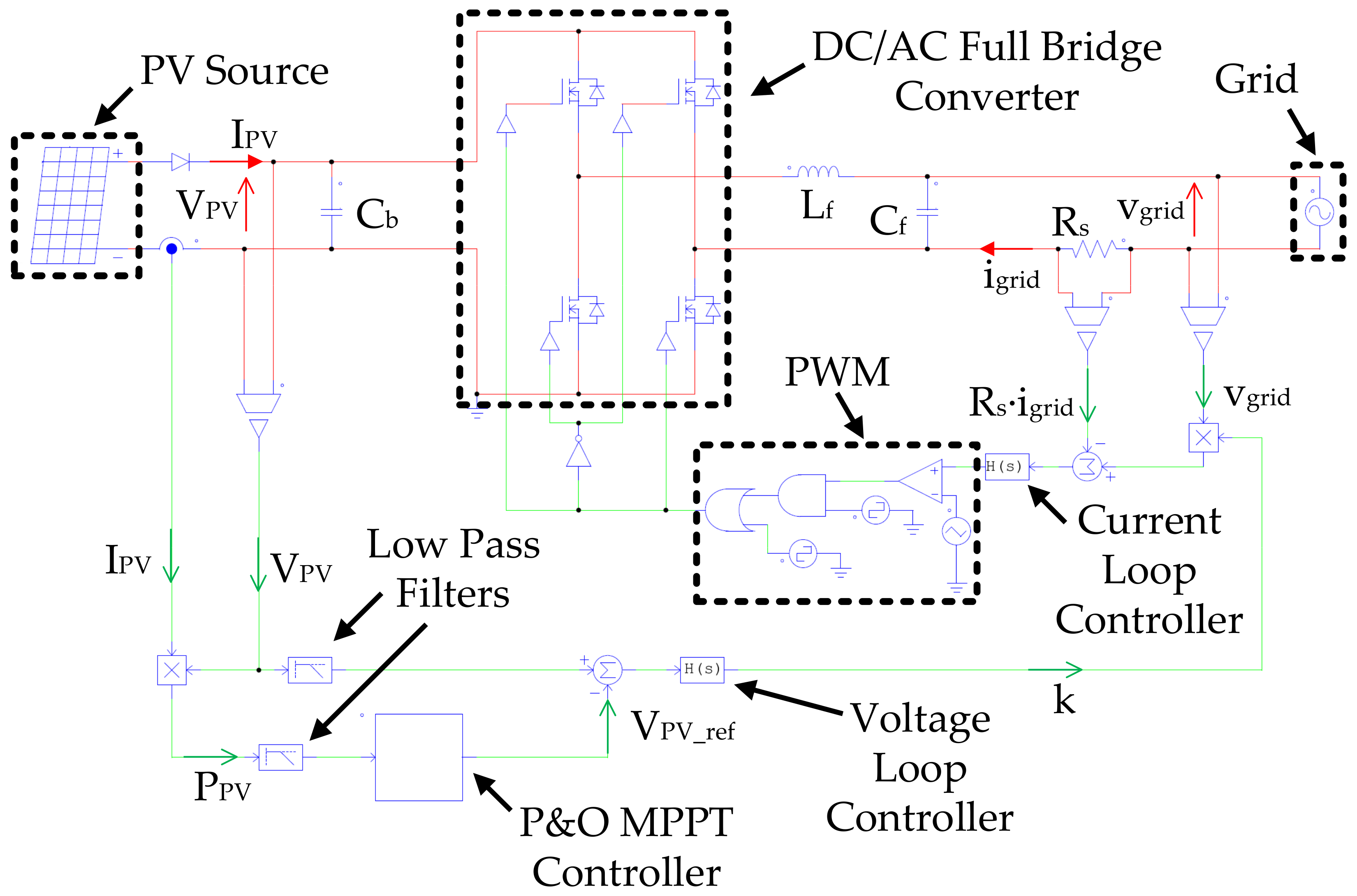
A typical single-stage grid-connected PV system is shown in
Figure 1 [
13,
14,
15]. The DC/AC converter is an active full bridge with a control circuitry exhibiting the presence of two control loops, an inner current control loop, and an outer voltage control loop [
16,
17].
A fast internal current control loop is aimed at injecting an AC current into the grid with a power factor ideally equal to one. The interested reader can find all the details concerning the proper design of such a control loop in [
16]. In this paper, ideal working of the internal current control loop (zero error) is assumed, and therefore the following equation represents the starting point for the analysis:
where R
s is the sensing resistance,
is the grid voltage, and f is the line frequency. It is worth noting that k(t) is a slowly varying signal [
16], hence from (1) it is possible to state that
, that is, i
grid(t) and v
grid(t) are in phase. The slowly varying signal, k, dictates the value of the average (over the period of the line frequency f) power, P
grid, injected into the grid, i.e., the higher the value of k, the higher the active power P
grid. In fact, it is
A slow external voltage control loop is aimed at the proper regulation of the PV voltage, V
PV. The reference voltage, V
PV_ref, is provided, as shown in
Figure 1, by the MPPT controller [
18,
19]. It is worth noting, as shown in
Figure 1, that two low-pass filters appear. One for the PV voltage, V
PV, and the other for the PV power, P
PV. Filtering is necessary in order to avoid errors of the MPPT technique, which can be deceived by the presence of harmonics (at the double of the line frequency and at the frequencies of switching harmonics). In addition, the working of the voltage control loop can be negatively affected by such harmonics. Henceforth, for brevity, we refer to V
PV and P
PV even if we indeed refer to their filtered versions.
As stated in the Introduction, the P&O technique is one of the most exploited MPPT techniques since it is simple but nonetheless very efficient. The P&O algorithm operates by periodically changing, step-by-step, the reference voltage, V
PV_ref, and by measuring the corresponding PV power, P
PV = V
PV·I
PV [
18]. After each perturbation of V
PV_ref, the P&O controller waits for the settling of the system steady-state and, subsequently, compares the new steady-state value of P
PV with the older one in order to drive the operating point towards the MPP. In particular, if after a perturbation of V
PV_ref the steady-state value of P
PV has increased (decreased), it means that the operating point has moved towards (away from) the MPP. Therefore, the next perturbation of V
PV_ref will have the same (opposite) sign as the previous perturbation, and so on. In summary, the control law that is implemented in the P&O MPPT controller of
Figure 1 is as follows:
where r is a growing integer index starting from 0 (r = 0, 1, 2, …). It is worth noting that in order to evaluate the PV extracted power, P
PV, appearing in (3), the PV current detection is necessary. Moreover, the objective of the P&O controller is the maximization of the power extracted by the PV source. Since the power stage efficiency η
power_stage(V
PV, P
grid) [
20,
21,
22,
23,
24,
25] is not taken into account, the maximization of the PV power does not necessarily correspond to the maximization of the power P
grid = P
PV∙η
power_stage(V
PV, P
grid) injected into the grid.
3. T4S MPPT Technique
As stated in the previous Section, k is a slowly varying signal [
16] which dictates the value of the average power, P
grid, in particular, the higher the k signal, the higher the amplitude of i
grid(t), and hence the higher the P
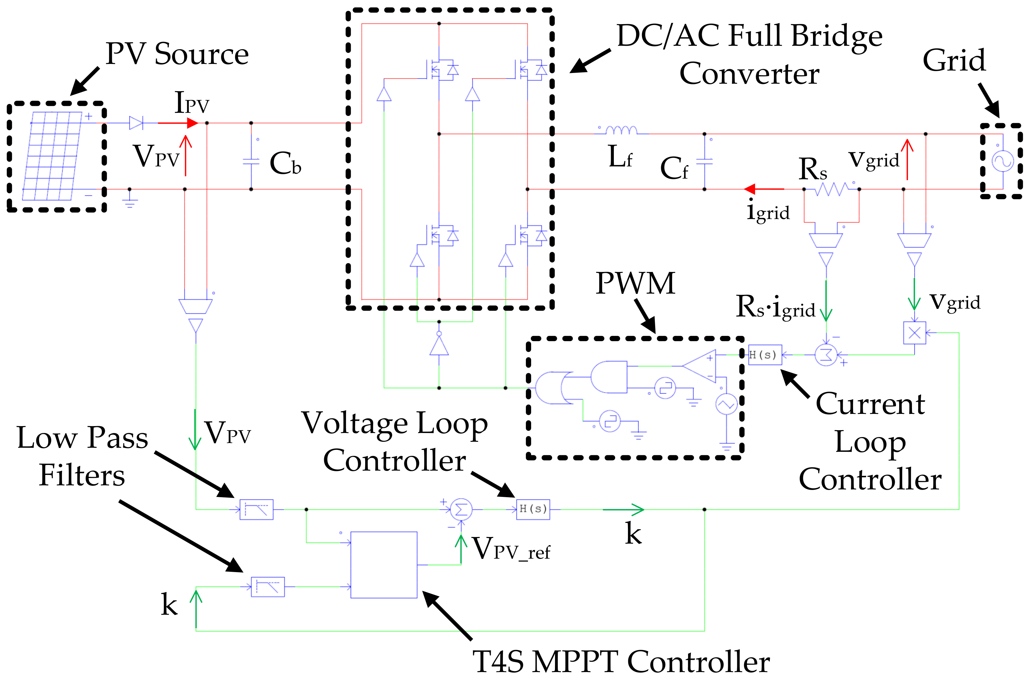
grid. On the basis of such a consideration, the objective of the proposed T4S MPPT technique is represented by the identification of the PV voltage reference, V
PV_ref, that leads to the maximization of the signal k. A single-stage grid-connected PV system equipped with the T4S MPPT controller is shown in
Figure 2. From
Figure 2, it is evident that for the T4S MPPT technique to function it needs only the sensing of the PV voltage, V
PV, and the signal k that is an already available internal signal. Even in this case, two low-pass filters appear and the same considerations, made with reference to
Figure 1, apply for the quantities, k and V
PV. It is worth noting, different from the P&O technique, that no PV current detection is necessary.
The operating principle of the T4S technique is well illustrated by the following control law that is implemented in the T4S controller of
Figure 2:
where K
I is a positive constant value and V
ref_0 is the initial value of V
PV_ref. In particular, the PV voltage reference, V
PV_ref, provided by the T4S controller is the output of an integrator, as shown in
Figure 3. Such an integrator processes a signal whose absolute value is the constant, K
I, and whose sign changes every T
SH second according to the sign of the product between the time derivatives of k and V
PV. Hence, V
PV_ref is a ramp function characterized by a slope equal to
.
In practice, the T4S MPPT technique is aimed at tracking the peak value of k with respect to V
PV since, as already evidenced above, the higher the value of the k signal, the higher the P
grid. Therefore, the output V
PV_ref of the T4S controller will have a positive slope (+K
I) in [r∙T
SH+, (r + 1)∙T
SH-] if k and V
PV are both increasing at t = r∙T
SH- (case A in
Figure 4a, where the operating point is located at the left of the MPP and is moving towards the MPP) or if k and V
PV are both decreasing at t = r∙T
SH- (case B in
Figure 4a, where the operating point is located at the left of the MPP and is moving away from the MPP). Instead, V
PV_ref will have a negative slope (-K
I) in [r∙T
SH+, (r + 1)∙T
SH-] if k is increasing and V
PV is decreasing at t = r∙T
SH- (case C in
Figure 4a where the operating point is located at the right of the MPP and it is moving towards the MPP) or if k is decreasing and V
PV is increasing (case D in
Figure 4a where the operating point is located at the right of the MPP and it is moving away from the MPP). In practice, the working of the T4S technique is based on the proper setting, every T
SH second, of the sign of the slope of the photovoltaic voltage reference signal, V
PV_ref, from which the name was chosen for the proposed MPPT technique.
At steady-state, in the neighborhood of the MPP, the T4S technique leads to a V
PV_ref waveform characterized by a piecewise ramp profile with a period equal to 2∙T
SH and a peak-peak amplitude equal to K
I∙T
SH (
Figure 4b). Hence, the steady-state performance of the T4S technique is strictly linked to the values assumed by the two parameters, T
SH and K
I. T
SH must be greater than the settling time of the filtered versions of the two input signals V
PV and k. Then, the proper value of K
I can be identified on the basis of the maximum allowed steady-state variation ΔV
PV = K
I∙T
SH of the PV operating point. It is worth noting that the higher the value of ΔV
PV, the higher the steady-state waste of available PV power.
4. Numerical Results
In this section, numerical results concerning the working of a grid-connected single-stage PV system equipped with a T4S MPPT controller are reported and discussed. In particular, the system, as shown in
Figure 2, has been implemented and tested in a PSIM environment [
26]. The RMS grid voltage, V
grid, was set equal to 230 V and the line frequency, f, was set equal to 50 Hz. The considered PV source is characterized, in STC, by P
MPP_STC = 3058 W and V
MPP_STC = 401.5 V. With regard to the current control loop, its crossover frequency, f
CI, was set equal to 5 kHz, and the switching frequency, f
SI, of the PWM modulator has been set equal to 50 kHz. Moreover, R
s = 0.1 Ω, C
b = 10 mF, L
f = 330 μH, and C
f = 47 μF. With respect to the slow voltage control loop, its crossover frequency, f
CV, was set equal to 5 Hz and the low pass filters cut-off frequency, f
LPF, was set equal to 10 Hz. The maximum allowed steady-state variation, ΔV
PV, of the PV operating point was set equal to 10 V; such a value leads to a maximum steady-state PV power waste equal to about 0.5%.
The parameters of the T4S technique were identified as explained in the previous section. In particular, in [
11] the interested reader can find a detailed analysis and discussion on the guidelines for the proper choice of perturbation periods in MPPT techniques with specific reference to the P&O technique. Basically, such perturbation periods must be greater than the system settling time in order to avoid errors in the MPPT process. In practice, the same considerations also hold for the proposed T4S MPPT technique. In particular, in the considered case, the estimated system settling time, to within 5%, is nearly equal to 0.26 s, which is consistent with the crossover frequency (5 Hz) of the voltage control loop. Therefore, T
SH = 0.4 s was selected. It is worth noting that the influence of the chosen value of T
SH on the performance of the proposed algorithm is such that, for a given K
I, the higher the T
SH the slower the tracking process under time-varying irradiance conditions and the higher the waste of available energy under steady-state irradiance conditions. Then, given the value of T
SH, the proper value of K
I can be identified on the basis of the maximum allowed steady-state variation, ΔV
PV = K
I∙T
SH, of the PV operating point, and, in particular, the higher the value of ΔV
PV, the higher the steady-state maximum waste of available PV power. Since ΔV
PV was set equal to 10 V, it is K
I = 25 V/s. Moreover, the starting value, V
ref_, of, V
PV_ref, was set equal to 450 V in order to ensure that, at the startup, the system works sufficiently far from the minimum allowed value of the DC input voltage of the full-bridge inverter that is equal to
. It is worth noting that because of the unit power stage efficiency of the power electronics interface of the ideal system implemented and simulated in PSIM, the maximum value of P
grid is only obtained when the PV source operates in its MPP.
4.1. Constant Irradiance
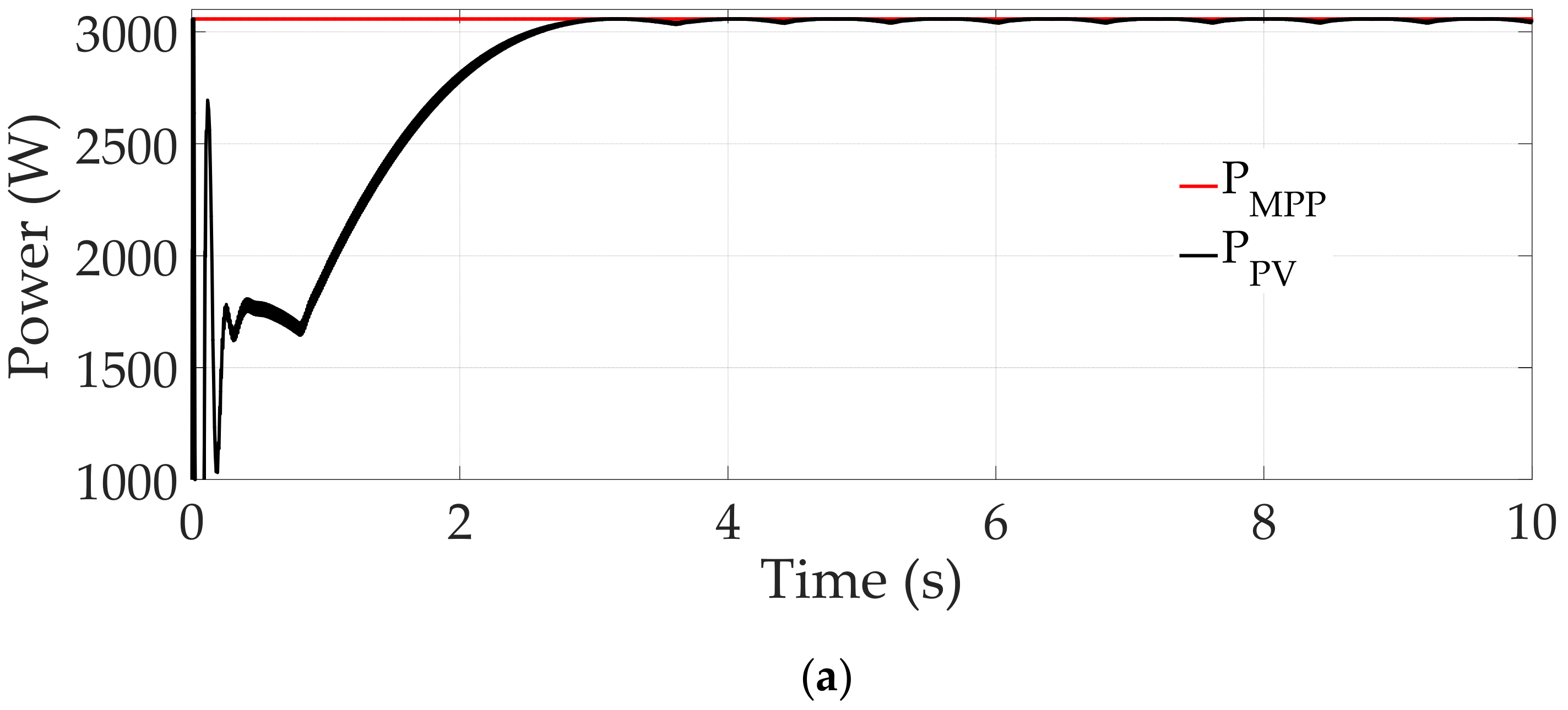
The first set of simulations were carried out in order to show the correct working of the proposed T4S MPPT technique and its ability to identify the maximum power point (MPP) under stationary irradiance conditions. In particular, a constant irradiance level, S = 1000 W/m2, was considered. In such a condition the PV source is characterized by PMPP = 3058 W and VMPP = 401.5 V.
The following figures illustrate the behavior of the technique at the startup. In particular, in
Figure 5 the PV extracted power is reported and compared with the available MPP power.
From the analysis of
Figure 5a, the ability of the proposed technique to identify, after about 4 s, the MPP without errors is evident. In
Figure 5b, a zoom of the steady-state behavior is reported. It is evident, as stated in the previous section, that the T4S technique leads to a periodic oscillation of the extracted power due to the periodic piecewise ramp profile of V
PV_ref, as shown in
Figure 6a. Moreover, as predicted, the maximum waste of power due to such an oscillation around the MPP is equal to about 0.5%, i.e., (3058 W – 3042 W)/3042 W, as shown in
Figure 5b, where 3058 W is the P
MPP and 3042 W represents the lowest level of the instantaneous extracted power. Moreover, from observations of
Figure 6b, it is clear, as explained in the previous Section, that the voltage, V
PV_ref, is characterized by a period equal to 2·T
SH = 0.8 s and a peak-peak amplitude equal to K
I·T
SH = 10 V.
4.2. Time-Varying Irradiance
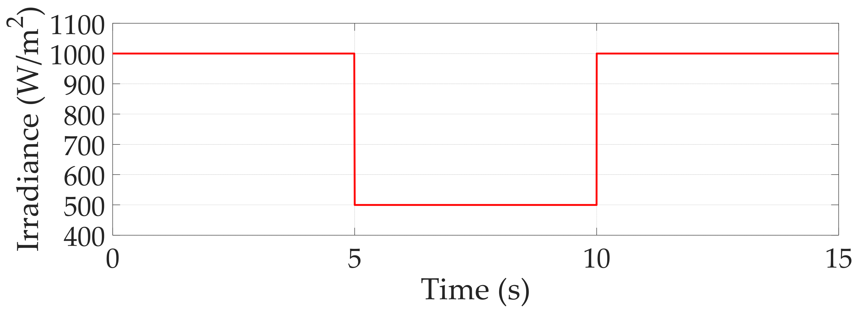
The second set of simulations were carried out in order to test the ability of the T4S MPPT technique to track the MPP under time-varying irradiance conditions. In particular, the operation of the T4S technique was tested by adopting the irradiance profile, as shown in
Figure 7. The considered irradiance exhibits a step change from S = 1000 W/m
2 to S = 500 W/m
2 at t = 5 s and back from S = 500 W/m
2 to S = 1000 W/m
2 at t = 10 s. At S = 1000 W/m
2, it is P
MPP = 3058 W and V
MPP = 401.5 V and at S = 500 W/m
2, it is P
MPP = 1598 W and V
MPP = 428 V.
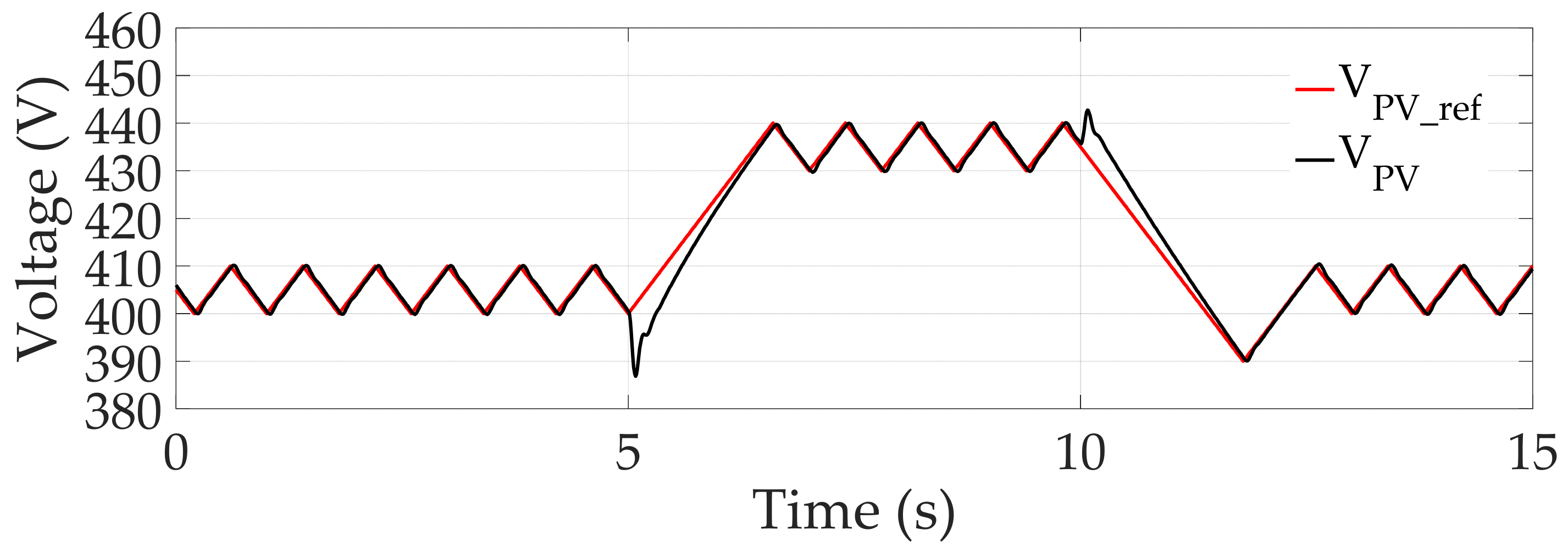
The results of the numerical tests under the time-varying irradiance profile shown in
Figure 7 are reported in the following figures. In particular, in
Figure 8, the PV extracted power is reported and compared with the available MPP power. In
Figure 9, the voltage, V
PV_ref, is reported together with the PV voltage, V
PV.
The previous figures show that the proposed MPPT technique is able to quickly track the MPP after any irradiance step variation.
5. Comparison between the T4S MPPT Technique and the P&O MPPT Technique
The last set of numerical tests were carried out in order to compare the performance of the proposed T4S MPPT technique with that of the traditional P&O algorithm. to this aim, the system shown in
Figure 1 was implemented and tested in a PSIM environment with the same values for the parameters as adopted in the previous section. The parameters of the P&O algorithm (T
P&O, ΔV
PV_ref, and V
ref_0) were chosen on the basis of the guidelines reported in the literature [
11] and in order to obtain the same steady-state maximum waste of power (0.5%) considered in the previous section, in particular, T
P&O = 0.4 s, ΔV
PV_ref = 10 V, and V
ref_0 = 450 V. It is worth noting that the values of the parameters that have been chosen for the P&O technique fully ensure a fair comparison with the T4S MPPT technique.
In the following, the symbol κ
d% indicates the quantity (P
T4S-d/P
P&O-d − 1)·100% where P
T4S-d is the average extracted power in dynamic conditions by adopting the T4S technique, and P
P&O-d is the average extracted power under the same dynamic conditions by adopting the P&O technique. “Dynamic conditions” mean working conditions taking place in the interval of time occurring between an event associated with a change of the irradiance conditions and the subsequent settling instant of steady-state periodic conditions. In particular, steady-state periodic conditions associated with the T4S technique are characterized by a piecewise ramp voltage behavior with period equal to 2·T
SH, as discussed in
Section 3 and reported in
Figure 4b. Instead, steady-state periodic conditions associated with the P&O technique are characterized by a three-level voltage behavior with period equal to 3·T
P&O [
11]. It is worth noting that since the settling instant is, in general, different for the two MPPT techniques, the highest settling instant will be considered for the evaluation of κ
d%. In addition, the symbol κ
ss% indicates the quantity (P
T4S-ss/P
P&O-ss − 1)·100%, where P
T4S-ss is the average extracted power in steady-state periodic conditions by adopting the T4S technique, for a given irradiance level, and P
P&O-ss is the average extracted power in steady-state periodic conditions by adopting the P&O technique for the same irradiance level.
5.1. Stationary Irradiance Conditions
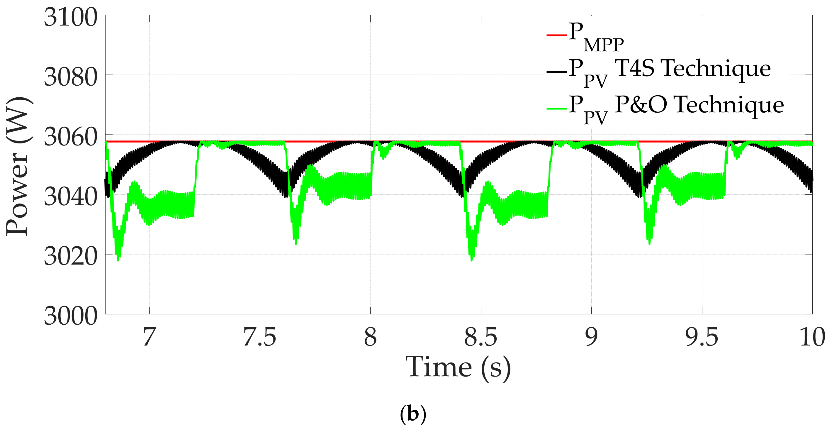
The powers extracted by adopting the T4S and the P&O MPPT techniques under a constant irradiance (S = 1000 W/m
2) are reported together in
Figure 10a. It is evident that both techniques need nearly the same time, at the start up, to reach the MPP. Such a startup can be seen as a step change of the irradiance level from 0 to 1000 W/m
2 and is characterized by a settling instant equal to 4 s, P
T4S-d = 2519 W, P
P&O-d = 2345 W, and hence κ
d% = 7.4%. In addition, by looking at the zoom of
Figure 10b, no remarkable difference in the steady-state efficiencies of the two MPPT techniques can be identified, although, indeed, the T4S performance is slightly better. In particular, P
T4S-ss = 3053 W, P
P&O-ss = 3048 W, and hence κ
ss% = 0.16%.
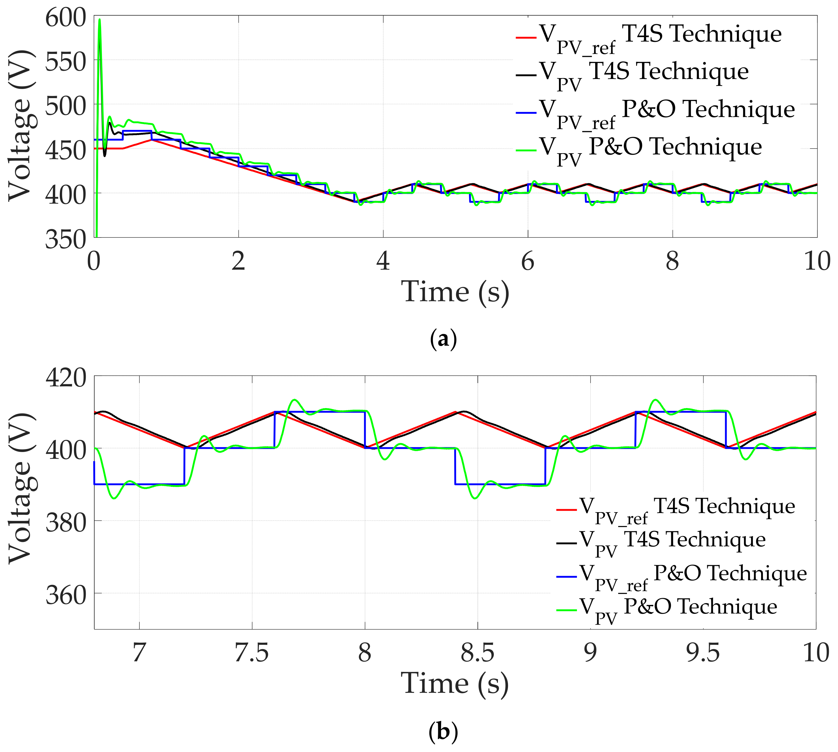
An interesting difference between the two MPPT techniques can be evidenced by observing
Figure 11a and, in particular, its zoom in
Figure 11b. In this figure, V
PV_ref and V
PV are reported for both of the MPPT techniques. It is clear for the P&O case, at steady-state, V
PV_ref ≈ V
PV oscillates around the MPP by assuming, as expected, the following three values: V
MPP - ΔV
PV, V
MPP, and V
MPP + ΔV
PV [
18]. Instead, in the T4S case, V
PV_ref ≈ V
PV exhibits a piecewise linear behavior with values belonging to the range [V
MPP and V
MPP + ΔV
PV]. In other words, the T4S operating point is always located at the right of the MPP.
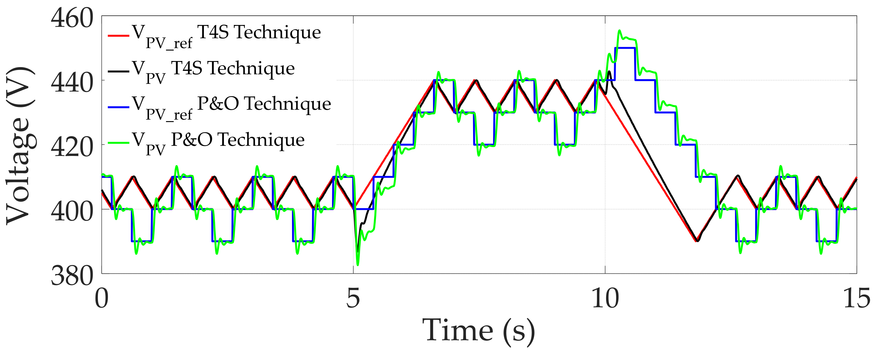
5.2. Time-Varying Irradiance
The performances of the two MPPT techniques were compared also under time-varying irradiance conditions. The adopted time-varying irradiance profile is shown in
Figure 7. The powers extracted by adopting the T4S and the P&O MPPT techniques under such an irradiance profile are reported together in
Figure 12. In
Figure 13, V
PV_ref and V
PV are reported for both of the MPPT techniques. From the abovementioned figures, it is evident the P&O MPPT technique is outperformed by the T4S technique, at least in correspondence to the irradiance positive step.
From the above figures, it is evident the P&O MPPT technique is outperformed by the T4S technique, at least in correspondence to the irradiance positive step. In particular, in correspondence of the irradiance negative step occurring at t = 5 s the following values have been obtained: settling instant equal to 6.2 s, PT4S-d = 1571 W, PP&O-d = 1561 W, and hence κd% = 0.64%. In correspondence to the irradiance positive step occurring at t = 10 s the following values have been obtained: settling instant equal to 12.2 s, PT4S-d = 2971 W, PP&O-d = 2721 W, and hence κd% = 9.2%.


