An Accurate, Light-Weight Wind Speed Predictor for Renewable Energy Management Systems

Abstract

This paper proposes an approach for accurate wind speed forecasting. While previous works have proposed approaches that have either underperformed in accuracy or were too computationally intensive, the work described in this paper was implemented using a computationally efficient model. This model provides wind speed nowcasting using a combination of perturbed observation ensemble networks and artificial neural networks. The model was validated and evaluated via simulation using data that were measured from wind masts. The simulation results show that the proposed model improved the normalized root mean square error by 20.9% compared to other contending approaches. In terms of prediction interval coverage probability, our proposed model shows a 17.8% improvement, all while using a smaller number of neural networks. Furthermore, the proposed model has an execution time that is one order of magnitude faster than other contenders.

1. Introduction

Renewable energy sources (RES) are sustainable resources that can help in alleviating the environmental pollution caused by fossil fuels. In fact, many consider RES as one of the key solutions to the energy crisis. The latter was exacerbated by the decrease in the supply of fossil fuel energy due to the shortage of these resources [1]. Therefore, both environmental concerns and the energy crisis have motivated a rapid adoption of renewable and sustainable sources of energy.

In particular, wind energy is considered as one of the most important and reliable renewable resources to depend on [2,3]. The reliance on wind energy has increased worldwide and is expected to flourish even further in the near future [2]. However, the main challenge that may impede the global adoption of wind energy is the unpredictability of wind speed [4]. Without an accurate prediction of wind speed, it will be very difficult to estimate the power generated from wind farms. As a result, power dispatching utilities will be unable to make commitments to the electrical grid from these wind farms.

Typically speaking, wind power scheduling is performed through a bidding process. In this process, RES power suppliers commit to power distribution companies to provide some amount of power at a specific time of the upcoming hour or day. For example, in the case of day-ahead scheduling, the commitment is made for the next day, while in spot markets, the next day's agreements are adjusted for the near future (i.e., 10 min to 6 h ahead) [3,5]. In such scenarios, a wind speed nowcast (i.e., short-term forecast) is required. Accurate wind speed nowcasting can play a vital role in accelerating the global integration of wind energy into the power grid.

Several approaches have been proposed in the last few decades to predict wind speed. However, many of these approaches are unsuitable for short-term prediction. On the other hand, some of the approaches that were tailored for short-term forecasting are not highly accurate in their predictions. Others are computationally expensive, and therefore, cannot be used in real time applications.

On the other hand, the last few years have witnessed an increasing interest in artificial neural networks. These networks can be trained to learn patterns, which can be used later for classification purposes. An interesting variation of artificial neural networks was suggested by Galmarini et al. [6], where the authors have proposed an approach that is currently referred to as “ensemble forecasting”. In essence, the approach suggests creating multiple instances of the network in order to obtain an aggregated decision. This aggregated decision is claimed to be better than any of the single-prediction methods.

Ensemble forecasting may help in improving the prediction accuracy. However, by itself, ensemble forecasting can do little in coping with uncertainties in the input dataset. This may place a cap on the ability of ensemble forecasting in improving the accuracy. Instead, one could argue that ensemble forecasting could be combined with another technique in order to remove such a cap.

The authors of this paper suggest the use of an additional technique that is capable of handling input uncertainties. Basically, several unique observations out of the original observation are constructed. These unique observations, widely known as perturbed observations, are constructed in such a way that they cover the uncertainties, and hence, support ensemble forecasting in achieving highly accurate predictions.

Therefore, the main objective of this paper is to develop a model that combines ensemble neural networks with perturbed observations in order to boost the accuracy of wind speed prediction. The paper makes the following contributions:

• The paper investigates configurations of nonlinear auto-regressive with exogenous input (NARX) models that would yield accurate short-term wind speed predictions.
• The paper describes procedures for constructing perturbed observations using computationally efficient techniques. This will help in reducing the execution time of the proposed model, while maintaining the desired accuracy.
• The proposed model was benchmarked via simulation against other contenders using measured parameters that were recorded from a wind mast dedicated to a wind power generation plant. The model was found to improve the performance in terms of increasing the correlation and reducing the error.
• The proposed model was proven to execute much faster than other contenders (i.e., light-weight models).
• The proposed model provides probabilistic nowcasting information, which will help dispatchers to schedule ahead and make necessary adjustments based on the expected amount of output power from the wind farm in the spot market.
• Finally, the paper provides estimates of the generated power using a wake model of the actual wind farm.

The rest of this paper is structured as follows. Section 2 provides a literature review and a background of relevant topics. Section 3 presents the proposed model for wind speed prediction, followed by a description of the simulation model in Section 4. The results are discussed in Section 5, while Section 6 concludes the paper with final remarks and suggested future directions.

2. Literature Review and Background

2.1. Wind Speed Prediction

There are a number of methods that are used to predict wind speed. The persistence method, for example, assumes that an event such as wind speed at a certain future time will be the same as of now [7]. This class of methods is more suitable for very short-term forecasting, given that as time steps are increased, the accuracy of the persistence method gradually decreases [8]. On the other hand, physical methods are mathematical models that use physical parameters such as land surfaces, obstacles, temperature, pressure measurements, etc., to make the best possible prediction for a certain event. Given their computational complexity, this class of methods is unfit for short-term predictions (i.e., those <6 h ahead), as it requires high performance machines to process complex mathematical models [9,10]. On the other hand, statistical methods rely on historical data to formulate the mathematical model that is used to perform the predictions. These methods can be further divided into two models, namely, the conventional time series and artificial neural network (ANN) models. These models are good for short-term predictions and are computationally inexpensive, as they do not require high performance computing [3]. In particular, ANNs possess an excellent ability in learning from previous data. These neural networks are highly accurate and run faster on machines than other approaches in this context [2].

ANNs in general, and recurrent neural networks (RNNs) in particular, are considered by many as the most suited methods to forecast wind speed. These non-linear models are more efficient in capturing the input-output relationship and generalize faster to perform the prediction [11,12,13]. Interestingly, RNNs include feedback signals from the hidden and output layers back to the input layer. This allows temporal information to be effectively represented and operated on. In contrast to traditional feed-forward neural network models, RNNs can establish a dynamic mapping that links the input to the output sequences. The most common RNN model that is used to perform short-term wind speed forecasting is the nonlinear auto-regressive with exogenous input (NARX) model. This neural network model is used in time series predictions, where it converges faster, compared to other ANNs, in the time series domain and produces optimal results with high accuracy in terms of a low mean square error (MSE) [14,15].

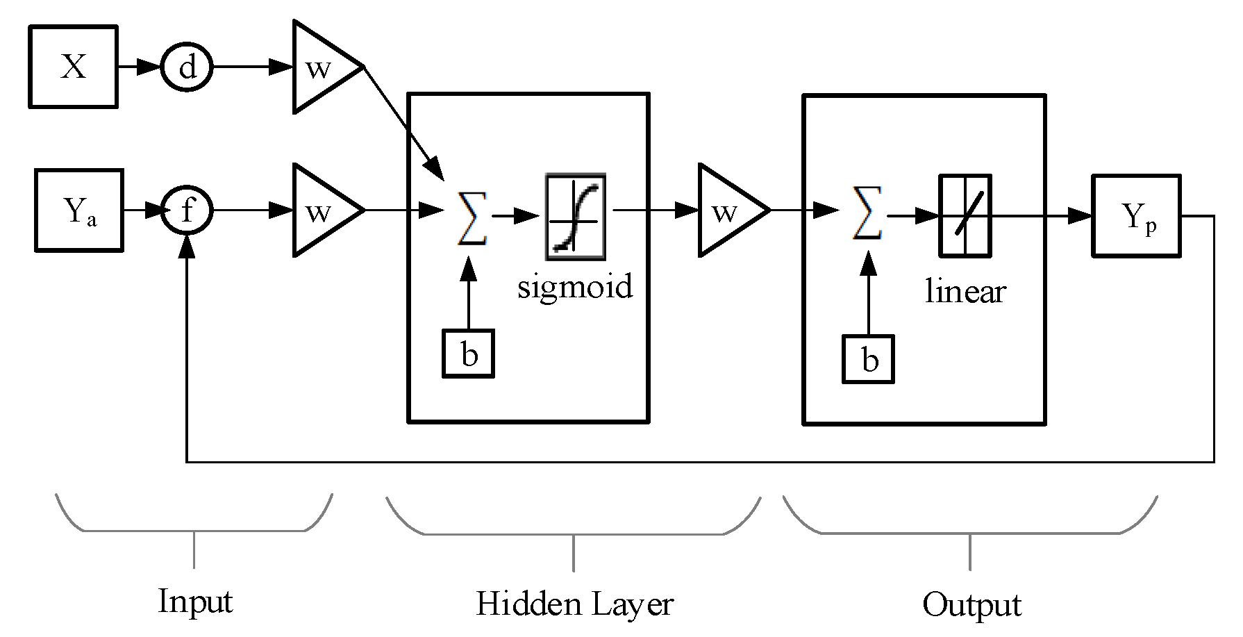
NARX is a non-linear recurrent dynamic neural network, with feedback connections from the output layer back to the input layer. What is special about this model is that it accepts external (exogenous) inputs to the system. Therefore, the adaptive learning process makes NARX well suited for time-series modeling, even with small scale data delays [16,17]. There are two types of NARX system architectures that are used in time series modeling, namely, series-parallel (open-loop) and parallel networks (closed-loop). As shown in Figure 1, the open-loop configuration uses the original dataset as an input instead of the estimated output. This network configuration is useful for training purposes [18,19].

The open-loop network configuration can be expressed as:

$$Y_p\left(i\right)=f\left(Y_a\left(i-1\right),Y_a\left(i-2\right),\dots ,Y_a\left(i-f\right),X\left(i-1\right),X\left(i-2\right),\dots ,X\left(i-d\right)\right)$$

(1)

where the predicted output $Y_p\left(i\right)$ is generated from the previous $f$ steps of the actual observations of the same event and the previous $d$ steps of the exogenous input $X$. The terms $f$ and $d$ represent the feedback and input delays, respectively. In contrast, the predicted output in the closed-loop configuration is fed back to the input layer, as depicted in Figure 2. This type of configuration is useful for multi-step-ahead prediction [18,19]. The closed-loop configuration can be mathematically expressed as follows:

$$Y_p\left(i+1\right)=f\left(Y_p\left(i\right),Y_a\left(i-1\right),\dots ,Y_a\left(i-\left(f-1\right)\right),X_p\left(i\right),X\left(i-1\right),\dots ,X\left(i-\left(d-1\right)\right)\right)$$

(2)

The equation shows that in multi-step-ahead predictions, one-step-ahead output $Y_p\left(i+1\right)$ depends on the previous $f-1$ observations of an event, $d-1$ exogenous input steps, one step back of the feedback prediction of the event $Y_p\left(i\right)$, and the predicted values of exogenous input $X_p\left(i\right)$.

2.2. Ensemble Forecasting

Ensemble forecasting is popular in applications that employ statistics and machine learning time series prediction. The obtained output from multiple members is an aggregated decision, which is better than any of the single-prediction methods [20]. In fact, the ensemble model was introduced in weather forecasting by Galmarini et al. [6], where it was shown that such models have the potential to improve the accuracy of forecasting.

Generally speaking, the uncertainty in the forecasted values occurs due to two main reasons, namely, the initial conditions and model uncertainties [21]. The initial condition uncertainties refer to errors in measured parameters, missing data in the dataset, limited observations of the atmosphere, errors due to the measuring equipment (i.e., sensors), etc. On the other hand, the model uncertainty occurs due to errors in the network parameters, such as the architecture, initial weight selection, activation function selection, training algorithms, number of neurons in each layer, etc. These uncertainties can be used to improve the accuracy of the model by using them as ensemble members [22,23]. There are two ensemble forecasting methods, namely, parameter diversity and data diversity.

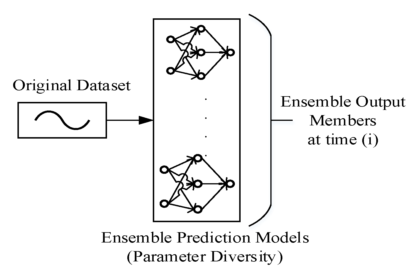
In the parameter diversity method, the ensemble predictor models differ from each other by having different parameter settings (e.g., different training algorithms, structure, activation function, or even prediction models) [23,24]. Figure 3 illustrates an ensemble prediction model that implements the parameter diversity method. In contrast, Figure 4 shows the data diversity method, where a different dataset for each ensemble predictor is used. The diversity in a dataset can be accomplished by having multiple observations for a certain event. Alternatively, data diversity can be achieved by processing the original dataset in a way that generates multiple subsets. The latter alternative is known as perturbed observations, which will be discussed in the following subsection.

2.3. Perturbed Observations

The main objective of this method is to generate several unique observations out of the original observation. The generated observations are created to cover the uncertainties, which may occur in the original dataset, leading to errors in the output predictions, as mentioned earlier. Perturbed observations ensemble models generate an ensemble of parallel forecasts for each data cycle, and the networks will differ from each other by having different input data. In each data cycle, a set of unique observations of multi-step-ahead predictions will be received from each model that is used in the ensemble network model. These observations are called ensemble members, which are used to calculate the final forecasted value in deterministic or probabilistic nowcasting forms. For instance, the observations can be generated by randomly adding a bias, as done in [25], where the process of obtaining the bias value is explained in [26].

Furthermore, the forecasting performance can be further improved by utilizing the bootstrapping method to handle data and model uncertainties. However, the ensemble network is a computationally intensive method, as it utilizes a large number of ensemble members running in parallel to forecast an event (e.g., 100 × 100 NARX models [27]). Moreover, the bootstrap method uses the MSE that resulted from the first batch ensemble networks in order to train the second batch of ensemble networks, which is impractical when attempting to provide multi-step-ahead forecasting.

3. Proposed Model and Methodology

As discussed earlier, perturbed ensemble networks approach can be used to improve the accuracy of a prediction model. In this study, the perturbed observations method is used to obtain multiple observation sets, which are used to train a number of NARX networks. This approach is inspired by the bootstrapping method [27,28,29,30,31]. The proposed approach will boost the performance of each ensemble neural network, leading to an improvement in the overall model’s accuracy. The reader is reminded that we are mainly interested in wind speed nowcasting (i.e., short-term prediction of wind speed).

3.1. Training Procedure

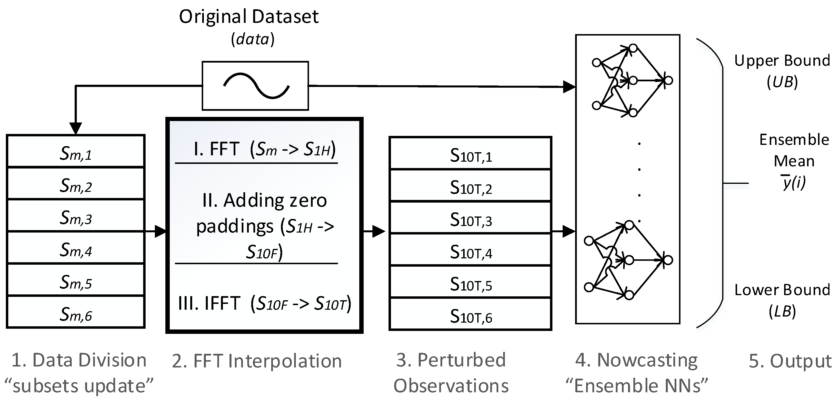
Figure 5 illustrates the proposed procedure for training the model. The procedure consists of four steps, which are described as follows:

• Data division: The measurements need to be fed to the network. These measurements are recorded periodically, where it is assumed that the measurements are recorded once every 10 min (i.e., in 10-minute intervals). This assumption is realistic and is compatible with actual datasets, including the one used in this work (to be discussed later). Henceforth, the measured data is referred to as the original dataset. Consider the dataset $data$, which is a collection of $n$ samples, such as $data=\left\{dat{a}_1,dat{a}_2,\cdots ,dat{a}_n\right\}$. The dataset is divided into several sub-datasets of 1-hour intervals each, as shown in Equation (3):

  $$\begin{gathered} S_{m,k}=\left\{dat{a}_k,dat{a}_{k+m},dat{a}_{k+2m},\cdots ,dat{a}_{n-m+k}\right\}; \\ \left\{k\in \mathbb{N}:1\le k\le m\right\} \end{gathered}$$

  (3)

  where $S_{m,k}$ are the subsets that are obtained from original dataset $data$, and $m$ is the number of perturbed ensemble networks. The subsets are formed by distributing the original data points sequentially, such that each 10-minute step point will be fed into a different subset.
• FFT interpolation: This step generates a number of subsets from the original dataset, resulting in the construction of perturbed observations for ensemble networks. In other words, fast Fourier transform (FFT) interpolation is applied to the subsets that were obtained from the previous step in order to generate six new subsets, where each subset consists of 10-minute interval measurements (i.e., perturbed observations).
  The subsets $S_m$ of length N are transformed from the time domain to $S_{1H}$ in the frequency domain using FFT, as expressed in Equation (4):

  $$\begin{gathered} S_{1H}\left(k\right)={{\displaystyle \sum }}_{j=1}^n{S}_{\text{m}}\left(j\right)W_n^{\left(j-1\right)\left(k-1\right)}; \\ {W}_n=e^{-2\pi /n} \end{gathered}$$

  (4)
  Then, zero paddings will be applied to increase the length of$S_{1H}$, from N to$L=N+M\left(N-1\right)$, where $M$ is the number of data points that will be added between every two known points in the subsets. This study uses $M=5$. Therefore, there is a need to estimate the 5-point missing data between every two known points in 1-hour subsets,$S_{1H}$, to extract datasets $S_{10F}$ with length $L$.
  Then, inverse FFT is applied to the frequency domain signals $S_{10F}$ to transform them back to time domain$S_{10T}$. This can be represented mathematically as follows:

  $$\begin{gathered} S_{10T}\left(j\right)=\frac{1}{n}{{\displaystyle \sum }}_{k=1}^n{S}_{10F}\left(k\right)W_n^{-\left(j-1\right)\left(k-1\right)}; \\ {W}_n=e^{-2\pi /n} \end{gathered}$$

  (5)
  $S_{10T}$ represents the 10-minute interval datasets in the time domain, which basically constitute the perturbed observations.
• Perturbed observations: The previous step has produced six perturbed, 10-minute interval observations. These are fed to the ensemble neural networks for training.
• Training ensemble neural networks: The ensemble network consists of 7 NARX neural networks, where six ensemble networks were trained using the perturbed observations and one network was trained using the original dataset.

3.2. Nowcasting Procedure

A similar procedure to the training was also developed for nowcasting, as shown in Figure 6.

The steps are listed below:

• Data division: Every 10 min, the subsets are updated with a new data point from the original observation dataset.
• FFT interpolation: The perturbed observations are constructed from the subsets, as described previously. This will result in restoring six new subsets of 10-minute intervals.
• Perturbed observations: Six perturbed observations were obtained, each of which is a 10-minute interval. These are fed to the ensemble neural networks.
• Nowcasting: The NARX networks that were trained in the previous section are used to perform multi-step-ahead nowcasting.
• Output: Both deterministic and probabilistic nowcasting can be derived from the output of the model. The deterministic nowcasting can support the power dispatching systems to estimate the amount of the future output power from the wind farm. In contrast, the probabilistic nowcasting provides additional information about the worst case scenarios (e.g., the minimum expected output power), which can help in decision making when it comes to making commitments to the electrical grid.

The deterministic output is calculated by taking the average of the outputs of the ensemble networks:

$$\overline{y}\left(i\right)=\frac{1}{n}{\displaystyle \sum }_{k=1}^n{\tilde{y}}_k\left(i\right)$$

(6)

where $\overline{y}\left(i\right)$ is the output of the ensemble networks at time $i$. The ensemble members ${\tilde{y}}_k\left(i\right)$ are the output from each NARX in the ensemble model, and $n$ is the number of ensemble NARX networks.

On the other hand, the probabilistic nowcasting information was obtained by constructing a prediction interval (PI). The PI provides the range, which contains the upper bound “$UB$” and the lower bound “$LB$” of the nowcasted value. This range was obtained with a 95% confidence level, which the nowcasted value is estimated to fall in. The upper and lower bounds are calculated for each nowcasted value as follows:

$$UB\left(i\right)=\overline{y}\left(i\right)+{\mathrm{t}}_{1-\mathsf{\alpha }}·STD\left(i\right)·\sqrt{1+\frac{1}{n}}$$

(7)

$$LB\left(i\right)=\overline{y}\left(i\right)-{\mathrm{t}}_{1-\mathsf{\alpha }}·STD\left(i\right)·\sqrt{1+\frac{1}{n}}$$

(8)

where $LB\left(i\right)$ and $UB\left(i\right)$ represent the lower and upper bounds of the PI, respectively. The parameter ${\mathrm{t}}_{1-\propto }$ is the critical value probability distribution of the confidence level (1−α). $STD\left(i\right)$ is the standard deviation of the ensemble members, which is calculated using Equation (9):

$$STD\left(i\right)=\sqrt{\sigma {\left(i\right)}^2}=\frac{1}{n-1}{\displaystyle \sum }_{k=1}^n{\left(\overline{y}\left(i\right)-{\tilde{y}}_k\left(i\right)\right)}^2$$

(9)

3.3. Performance Evaluation of the Model’s Output

The performance of the deterministic nowcasting can be measured using the normalized root mean square error (nRMSE) and the Correlation Coefficient (R) [32]. These two metrics are used to express the discrepancy between the targeted value and the predicted output of the model. Equation (11) is used to express the nRMSE:

$$\mathrm{nRMSE}=\frac{1}{T}\sqrt{\frac{1}{N}{\displaystyle \sum }_{i=1}^N{\left(\overline{y}\left(i\right)-y\left(i\right)\right)}^2}$$

(10)

where $N$ is the number of predicted samples and $T$ is the range of the target observations and is expressed as follows:

$$T=WindSpee{d}_{MAX}-WindSpee{d}_{MIN}$$

(11)

Similarly, the correlation coefficient can be expressed as follows:

$$R=\frac{N{{\displaystyle \sum }}^{\text{}}{\left(\overline{y}\left(i\right)-y\left(i\right)\right)}^2-\left({{\displaystyle \sum }}^{\text{}}\overline{y}\left(i\right)\right)\left({{\displaystyle \sum }}^{\text{}}y\left(i\right)\right)}{\sqrt{N{{\displaystyle \sum }}^{\text{}}\overline{y}{\left(i\right)}^2-{\left({{\displaystyle \sum }}^{\text{}}\overline{y}\left(i\right)\right)}^2}\sqrt{N{{\displaystyle \sum }}^{\text{}}y{\left(i\right)}^2-{\left({{\displaystyle \sum }}^{\text{}}y\left(i\right)\right)}^2}}$$

(12)

Likewise, the probabilistic nowcasting of the ensemble models is evaluated in terms of reliability and sharpness using the prediction interval coverage probability (PICP) and the prediction interval normalized average width (PINAW). PICP is used to obtain the percentage of the targeted values that are covered by the PI. In contrast, PINAW provides information about the width of the interval [33,34]. The reliability (PICP) and sharpness (PINAW) are defined in Equations (13) and (14), respectively.

$$\mathrm{PICP}=\frac{1}{N}{{\displaystyle \sum }}^{\text{}}{C}_i;C_i=\{\begin{array}{c}1,y\left(i\right)\in \mathrm{PI}\\ 0,y\left(i\right)\notin \mathrm{PI}\end{array}$$

(13)

$$\mathrm{PINAW}=\frac{1}{N·r}{{\displaystyle \sum }}^{\text{}}\left(UB\left(i\right)-LB\left(i\right)\right)$$

(14)

where the coverage coefficient $C_i$ is equal to 1 if the predicted value is covered by the $\mathrm{PI}$ at a time $i$ (i.e., within [$UB\left(i\right),LB\left(i\right)]$bounds), and 0 otherwise.

3.4. Estimation of Wind Farm Power Output

The kinetic energy content of an air mass is proportional to its speed and mass. When a flowing air mass (wind) hits the blades of a wind turbine, it transfers part of its kinetic energy to the wind turbine and causes it to rotate. The reduction in the kinetic energy of the air mass is exhibited as a reduction of its speed and consequently pressure, immediately after the encountering the wind turbine blades. The difference between the air mass pressure and the atmosphere pressure decays as it moves away from the wind turbine, and it becomes negligible at sufficiently long distance from the turbine. Therefore, in a wind farm, the wind speed for downstream wind turbines may be affected by upstream wind turbines. This is referred to as the wake effect of the upstream wind turbine. Several models have been proposed to mimic the wake effect with different levels of accuracy and for use in certain applications [35,36,37,38,39]. A simple yet widely accepted model is the Jensen wake model developed by Jensen [35] and expanded by Katic et al. [36]. In the Jensen model, the decaying wake effect is modeled by a linear expansion of the affected area by the wind turbine wake for which the momentum remains constant [35]. 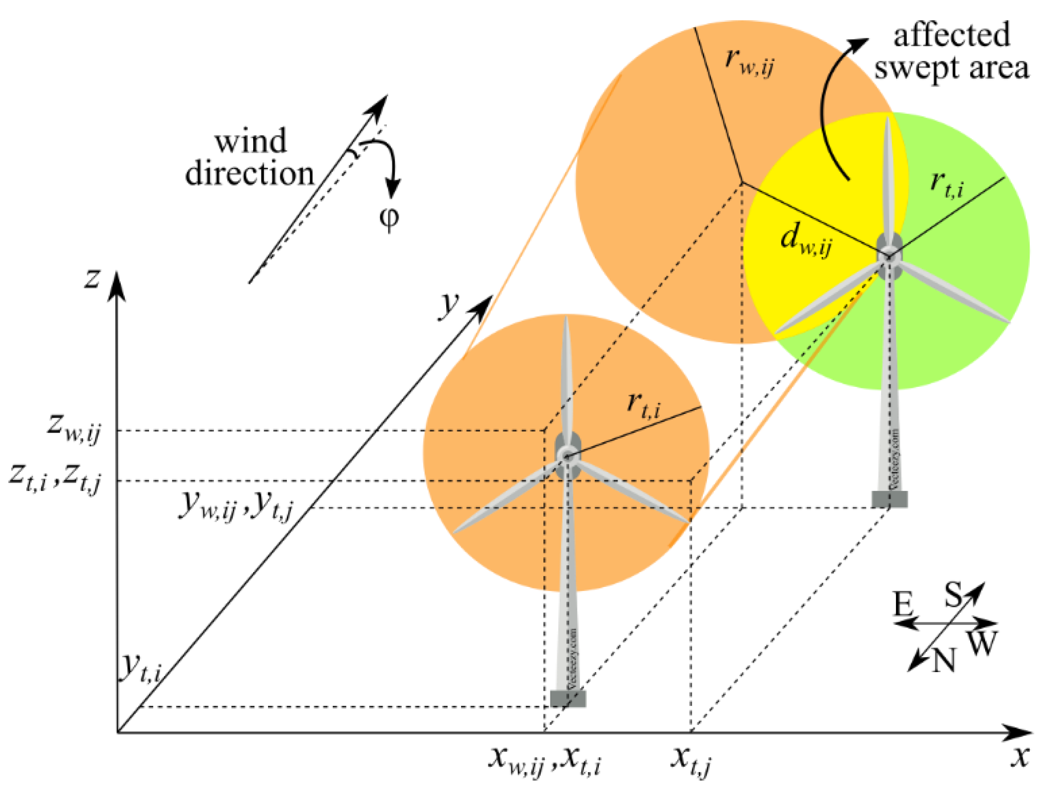Figure 7 shows two hypothetical turbines in a wind farm. Part of the swept area of wind turbine $j$ is under the wake effect of wind turbine $i$ when the wind direction is from north to south ($\theta =0$) and the wind flow angle is $\phi$.

Based on the Jensen model for a wind farm, the wind speed for wind turbine $j$ can be calculated by superimposing the wake effect of all other wind turbines $i$ [40]:

$$v_{t,j}=v_f\left(1-\sqrt{{\displaystyle \sum }_{\begin{array}{c}i=1\\ i\ne j\end{array}}^I{b}_i{a}_i^2{\psi }_{w,ij}^2}\right){\psi }_{h,j}$$

(15)

where $i$, $j$ $\in \left\{1,2,\dots ,I\right\}$ and $b$ is a binary parameter representing the status of the wind turbine (where 1 and 0 correspond to when the wind turbine is in or out of service, respectively). The other parameters are expressed in the Equations (16)–(19).

$$a_i=1-\sqrt[3]{{\left(1-0.5C_{T,i}\left(v_{t,i}\right)\right)}^2}$$

(16)

$${\psi }_{w,ij}=\frac{S_{w,ij}}{\pi r_{t,j}^2{\left(1+\frac{{\alpha }_i\left(y_{t,j}-y_{t,i}\right)}{r_{t,j}}\right)}^2}$$

(17)

$${\psi }_{h,j}=\left(\frac{log\frac{z_{t,j}}{\rho }}{log\frac{z_f}{\rho }}\right)$$

(18)

$${\alpha }_i=\frac{0.5}{log\frac{z_i}{\rho }}$$

(19)

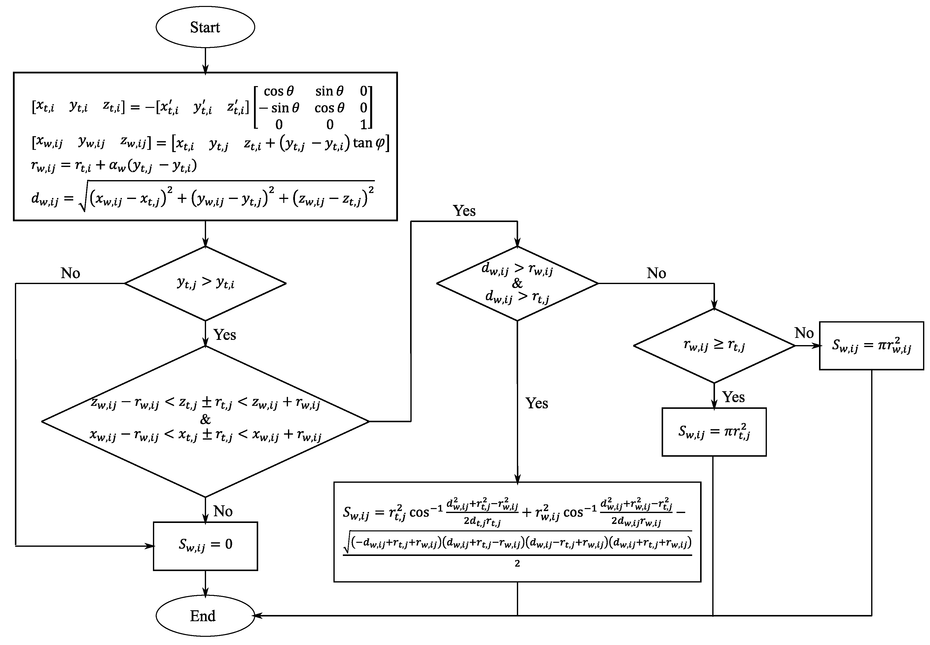
The affected wind turbine swept area $S_{w,ij}$ is calculated using the algorithm shown in Figure 8, where ($x_t^{\prime }$, $y_t^{\prime }$), $z_t^{\prime }$, and $r_t$ are the locus, height, and radius of the wind turbine, respectively. The thrust coefficient $C_T$ is found by interpolating over the thrust coefficient-wind speed characteristic of the wind turbine.

Similarly, the power generated by each wind turbine $P_{t,j}$ is estimated by interpolating over the power-wind speed characteristic of the wind turbine. These values are used to calculate the power output of the wind farm. It should be noted that with this formulation it is essential to carry out the calculation of wind speed for every turbine in ascending order of $y_t$. Therefore, the estimated power is calculated as follows:

$$P={\displaystyle \sum }_{i=1}^I{b}_i{P}_{t,i}\left(v_{t,i}\right)$$

(20)

Equation (20) will be used in our simulations to estimate the generated power from a wind farm given the wind speed that was predicted using our proposed model.

4. Model Simulations

The wind speed nowcasting model was implemented and validated in MATLAB (2014b, MathWorks, Natick, MA, USA). As for the dataset, the authors used measured parameters from the "Dhofar Wind Project" in Harweel, Sultanate of Oman (See Figure 9). The dataset includes measurements of temperature, humidity, pressure, wind speed, etc. These measurements were recorded at different heights (e.g., 79 meters, 60 meters, 42 meters, etc.) during a time span from November 2013 to October 2015.

For this study, the average wind speed measurements at an 80 meters height were used. In addition, the temperature and pressure values at a 76 meters height were used as exogenous inputs for the NARX network. Moreover, the data cleaning process was performed by removing duplicated data, which constituted less than 0.5% of the whole dataset. Nearest neighbor interpolation was used to handle some of the unrecorded measurements, where the latter constituted around 2% of the whole dataset.

A subset of the dataset (from November 2013 to December 2014) was used to train the nowcasting model, while the rest of the data were used to validate the model’s accuracy. The validation was done for four seasons, namely, winter (Jan–Feb, 2015), spring (Mar–May, 2015), summer (Jun–Aug, 2015), and autumn (Sep–Oct, 2015).

In order to quantify the improvement gain of using ensemble networks, the deterministic and probabilistic outputs were evaluated separately. First, the wind speed predictions were obtained by applying the persistence method, while nowcasting was trained and performed using a single NARX network. The results from both methods were used as a benchmark, as will be shown later, to compare the deterministic outputs of proposed model. The parameters of the single-network NARX were tuned until optimal performance was obtained. A summary of these parameters is shown in

Table 1. Single-network NARX parameter set.

Network Parameters	NARX
Number of Layers	2 (default)
Delays	Feedback delay = 6 steps Input delay = 6 steps
Hidden Layer Neurons	10 (default)
Inputs	Wind speed at 80 m Temperature and pressure at 76 m
Nowcasting	Wind speed at 80 m
Training Algorithm	Levenberg–Marquardt
Data Division Function	Divide by blocks
Performance Goal (MSE)	NARX, wind speed (≤0.05 m/s)
Training Epoch	1000 (default)

.

Then, the ten ensemble NARX networks were trained with same original dataset and nowcasting was performed in order to evaluate the improvement, which can be gained by perturbing the input dataset. Finally, the probability nowcasting results were compared to the output of the 10-ensemble networks, as well as the 100-ensemble bootstrapping method (to be discussed in the following section).

5. Results and Discussion

5.1. Performance in terms of Accuracy and Execution Time

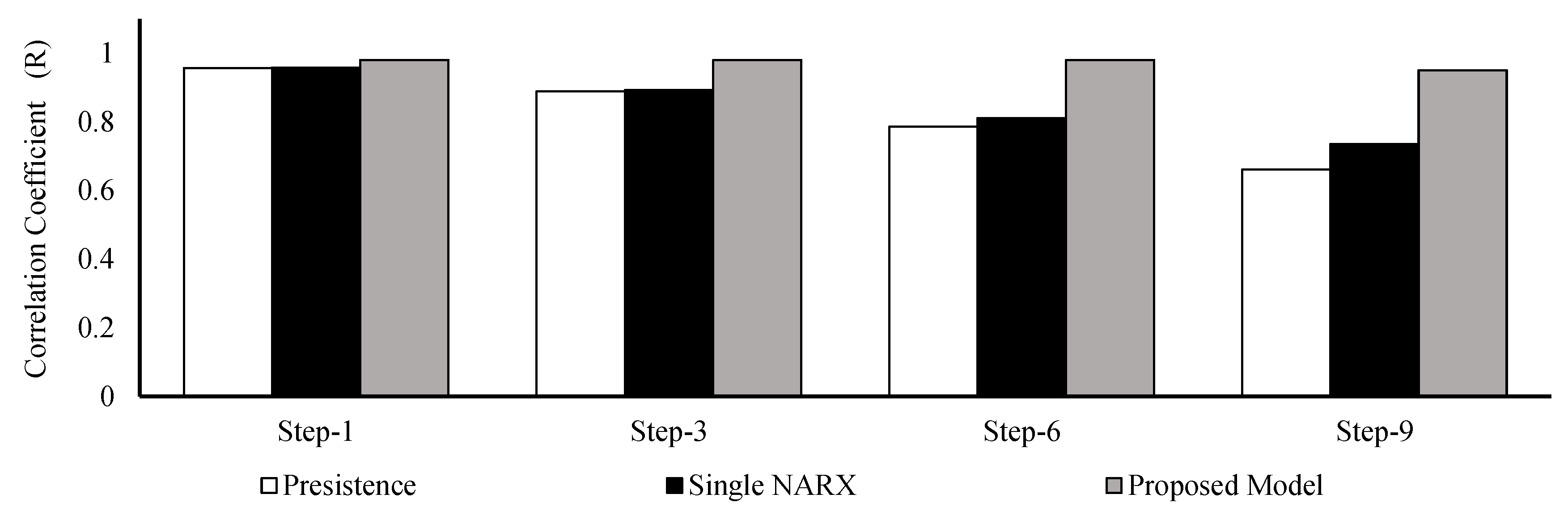
The deterministic nowcasting output was obtained by taking the average of the seven-ensemble members, where each member represents a NARX network output. Figure 10 shows the correlation coefficient (R) between the target values and the deterministic outputs. The figure shows a comparison between the proposed ensemble NARX, single-network NARX, and persistence models, using 500-step samples. The proposed model outperformed both the single-network NARX and the persistence model. The average performance of the proposed model has improved by 3% (from 95% to 98%) when compared to the single-network NARX model. What is more important is that the proposed model has improved the correlation of not only for the one-step-ahead nowcasting (i.e., 10-minute-ahead forecasting) but for all 9 steps (i.e., up to 90-minute-ahead forecasting).

Additionally, it is obvious from Figure 10 that the correlation between the target and the nowcasted output decreases as the prediction time steps expand along the horizon. For instance, the degradation in correlation between the 1- to 9-step predictions with the persistence model were the worst (30.9%), whereas the single-network NARX scored 23.25%. However, the proposed model was successful in maintaining the correlation by limiting the reduction by 3.06%.

Next, the performance of the proposed model was assessed by investigating the nRMSE. Figure 11 shows the evaluation of 500-step samples in terms of the nRMSE for the proposed model, in comparison to the single-network NARX and the persistence model. For one-step nowcasting, the proposed model performed better than the other two models by obtaining nRMSE of 0.024 m/s, whereas it was 0.0315 (0.0319) m/s for single-network NARX (persistence). This improvement is observed for all 9-step-ahead nowcasting.

Furthermore, it is expected that the accuracy of any prediction model will decrease as the prediction steps are increased. This is clearly visible in the case of the persistence and single-network NARX (See Figure 11), where the increase in nRMSE between steps 1 to 9 was 64% and 59.3%, respectively. In contrast, the proposed model has limited this growth to 43.15%, which is translated into an improvement of 20.9% compared to the persistence model.

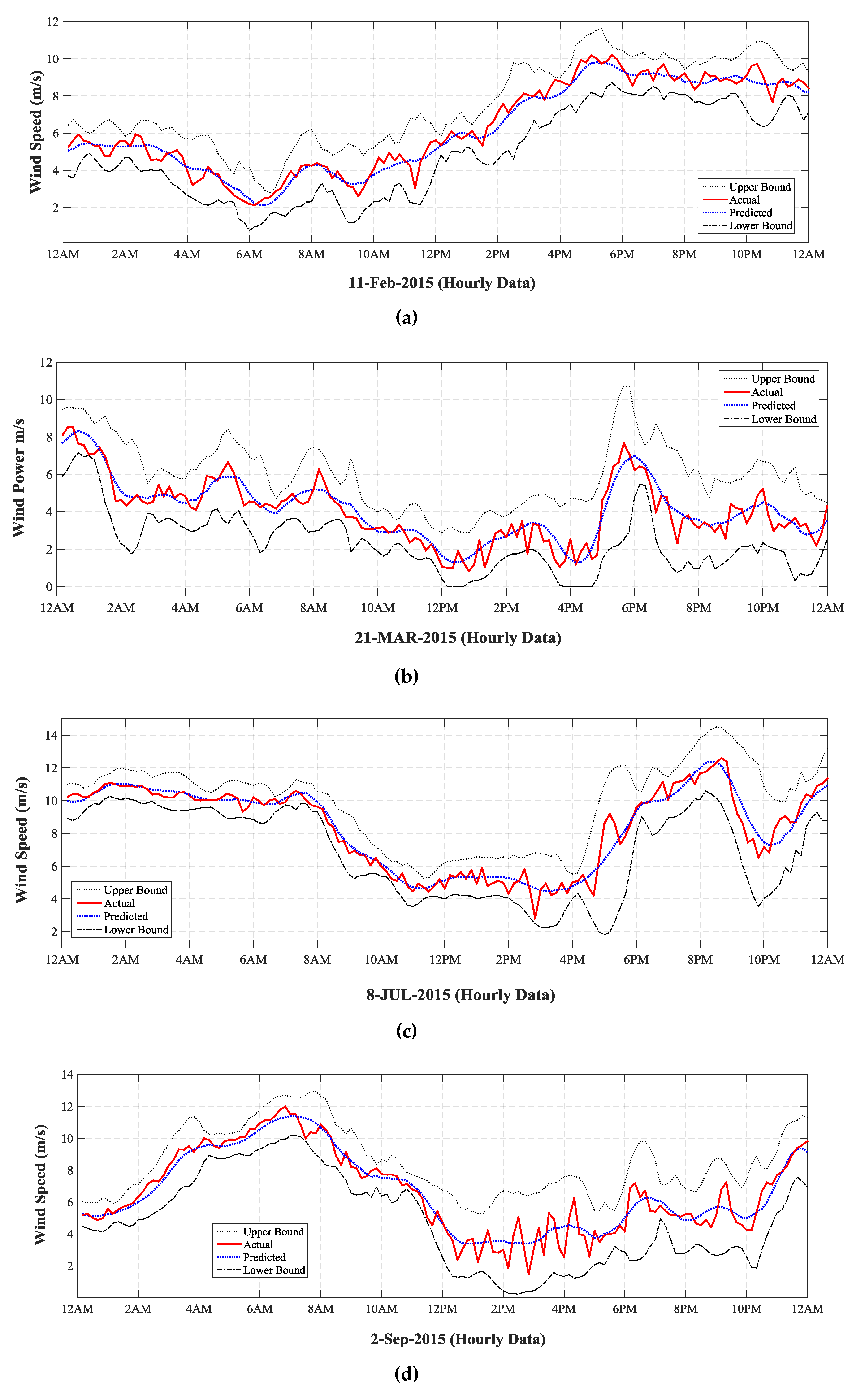
As discussed earlier, the probabilistic nowcasting is calculated using Equations (7)–(9). Figure 12 shows the 1-hour-ahead (i.e., 6-step-ahead) nowcasting output from the proposed model at different seasons. The curves in the figure represent the deterministic output from the ensemble model and the probabilistic lower/upper bounds, which were obtained at a 95% confidence level. The actual measurements were plotted in order to visualize the correlation with the deterministic output. The figure shows that the average PICP at 1-hour predictions for the ensemble NARX models was 99.7% for 500-steps samples. This means that 99.7% of the targeted values of wind speed dataset were covered under the predicted interval with a confidence of 95%. The good news is that even for 1.5-hour-ahead prediction (not shown in figure), the PICP is relatively high (97.3%).

The probabilistic nowcasting of the proposed 7-perturbed ensemble network was benchmarked against a 10-ensemble NARX network without perturbations and the model proposed by Anwar et al. [27]. To perform the evaluation, the RMSE and the PICP values at a 95% confidence level for the proposed model were calculated as 3-step-ahead (30-minute) predictions. Figure 13 shows the PICP evaluation for the proposed model compared to the benchmarks. It is observed that increasing the number of ensemble members from 10 to 100 has a positive impact on improving PICP. Anwar et al. [27] used 100-ensemble neural networks to improve the PICP by 14.2% when compared to the 10-ensemble neural network. In comparison, our proposed model uses a smaller number of networks while improving the PICP by 17.8% when compared to the 10-ensemble neural network.

Table 2. Prediction interval normalized average width (PINAW) for proposed model at different time steps (each step is 10 min).

Nowcasted Steps	PINAW (%)
1-step	12.11
3-step	13.66
6-step	17.29
9-step	21.42

shows the sharpness of the predicted interval, also known as the PINAW. In order to quantify the measure of sharpness, the nowcasted wind speed is used to estimate the generated power from the wind farm. This will be discussed in the following subsection.

The proposed model not only improves the prediction accuracy, but it is also less computationally intensive compared to the other contenders.

Table 3. A comparison of nowcasting execution time of proposed model vs. benchmarks.

Model	Time (s)/Sample
Bootstrap (100 NARX)	12.41
Ensemble (10 NARX)	0.77
Proposed Ensemble (7 NARX)	0.50

compares the execution time between the proposed model and the benchmarks. The execution time was obtained by running MATLAB simulations on a dual-core i5-7200U CPU operating at 2.50 GHz, with a total of 8 GB of physical memory. The table shows that the proposed model is one order of magnitude more computationally efficient compared to the bootstrap model. This is crucial, since these prediction models are expected to run continuously all day long, where real-time performance is favored.

5.2. Generated Power Estimation

Until now, the evaluation of the proposed model was restricted to measuring the correlation and error performance. However, integrating renewable energy sources such as wind into the electrical grid requires knowledge of the estimated energy that can be harvested during any time interval. This estimated knowledge is important for power dispatching utilities in order to make commitments to the grid. Therefore, it is essential to estimate the generated power from a wind farm using the wind speed that was predicted by the proposed model. This allows the assessment of the reliability of the model if it were to be integrated into a renewable energy management system.

To estimate the generated power, a 32.5 MW wind farm at Harweel, Oman, was modeled using a three-dimensional multi-speed and direction wake model [40], as discussed earlier. The Harweel wind farm layout, wind turbine characteristic [41], and the forecasted wind speed $v_f$ at height $z_f$ were used to estimate the power output (See Equation (20)). To focus solely on the wind speed forecasting, it was assumed that the wind direction was from north to south (i.e., $\theta =0\mathrm{rad}$, $\phi =0\mathrm{rad}$, and $b=1$) and the surface roughness length $\rho$ was 0.0005 m [42].

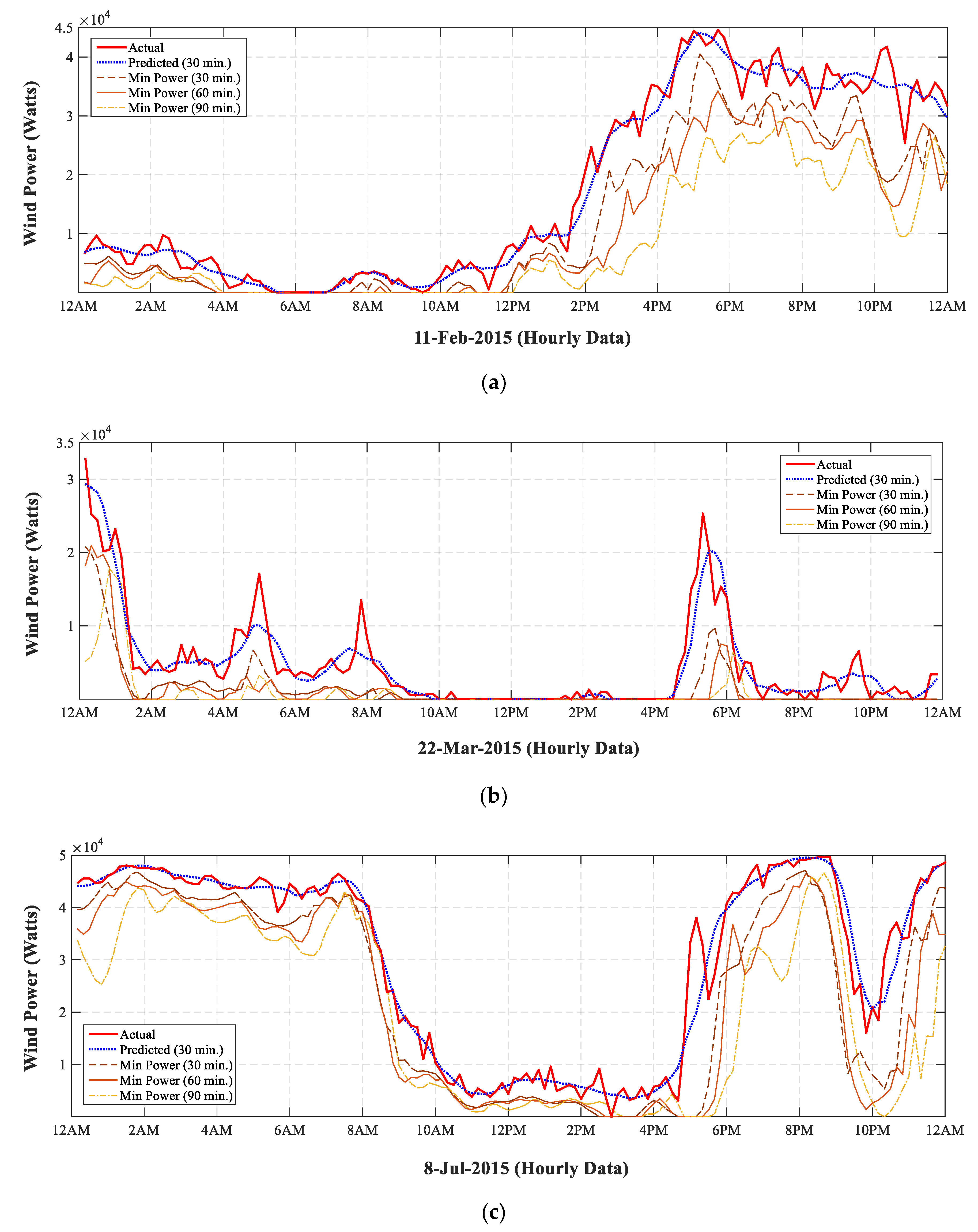
Figure 14 plots the actual generated power against the deterministic power prediction at 30 min ahead. In addition, the plot shows the minimum power output expectations at 1.5-hours, 1-hour, and 30-minutes ahead with a confidence of 95%. Providing expected minimum power output values every 10 min helps power dispatching systems to make the right decision when making commitments. For example, Figure 14a shows the estimated power on the 11th of February 2015. It is observed that the predicted wind speed, during the time from 4 AM to 12 PM, on that particular day, yielded lower power. However, an improvement is detected between 12 PM to 12 AM on that same day. These predictions are in fact in line with the actual wind activity, which will greatly help dispatch utilities in making commitments with lower risk.

6. Conclusions and Future Work

This study has proposed a novel method for predicting wind speed using ensemble networks fed with perturbed observations. The study used 7-ensemble NARX networks with perturbed observations. Actual measurements from a wind mast dedicated to a wind farm power plant were used in the simulations of the proposed model. The effectiveness of the proposed model was mainly attributed to introducing perturbed observations that were constructed from the original dataset using FFT interpolation. This resulted in multiple subsets for ensemble networks combined with NARX neural networks. The proposed perturbed ensemble NARX model outperformed the persistence and single-network NARX models in terms of the correlation between the targeted and predicted values and the error performance (nRMSE). In addition, the probabilistic nowcasting produced by the proposed model will help in minimizing risks while making commitments to the electrical grid.

The proposed ensemble model used a smaller number of networks while improving the PICP by 17.8% compared to 10-ensemble neural networks. Furthermore, the proposed model is superior in terms of the computational efficiency compared to the bootstrap method, where the latter requires hundreds of networks to run, while the former requires less than ten networks. As a result, the proposed model has a much faster execution time, and therefore, is more suitable for real-time applications.

The work done in this study has focused on predictions for a single wind farm. However, minor modifications are required when considering larger farm sizes, provided that relevant measurements are available. In fact, several works have indicated that increasing the farm area or grouping multi-farms together will help in reducing prediction errors [43,44,45]. Furthermore, the work presented in this paper can be further extended by considering the effect of wind direction on the potential harvested power from a wind farm.

References

- Manieniyan, V.; Thambidurai, M.; Selvakumar, R. Study on energy crisis and the future of fossil fuels. Proc. SHEE 2009, 10, 2234–3689. [Google Scholar]
- Lei, M.; Shiyan, L.; Chuanwen, J.; Hongling, L.; Yan, Z. A review on the forecasting of wind speed and generated power. Renew. Sustain. Energy Rev. 2009, 13, 915–920. [Google Scholar] [CrossRef]
- Soman, S.S.; Zareipour, H.; Malik, O.; Mandal, P. A Review of Wind Power and Wind Speed Forecasting Methods with Different Time Horizons. In Proceedings of the North American power symposium (NAPS), Arlington, TX, USA, 26–28 September 2010; pp. 1–8. [Google Scholar]
- Authority for Electricity Regulation, Oman. Study on Renewable Energy Resources, Oman; Authority for Electricity Regulation: Muscat, Oman, 2008. [Google Scholar]
- Krishna, V.B.; Wadman, W.S.; Kim, Y. NowCasting: Accurate and Precise Short-Term Wind Power Prediction using Hyperlocal Wind Forecasts. In Proceedings of the Ninth International Conference on Future Energy Systems, Karlsruhe, Germany, 12–15 June 2018; pp. 63–74. [Google Scholar]
- Galmarini, S.; Bianconi, R.; Bellasio, R.; Graziani, G. Forecasting the consequences of accidental releases of radionuclides in the atmosphere from ensemble dispersion modelling. J Environ Radioact. 2001, 57, 203–219. [Google Scholar] [CrossRef]
- Zhao, X.; Wang, S.; Li, T. Review of evaluation criteria and main methods of wind power forecasting. Energy Procedia 2011, 12, 761–769. [Google Scholar] [CrossRef]
- Wu, Y.-K.; Hong, J.-S. A Literature Review of Wind Forecasting Technology in the World. In Proceedings of the Power Tech, Lausanne, Switzerland, 1–5 July 2007; pp. 504–509. [Google Scholar]
- Potter, C.W.; Negnevitsky, M. Very short-term wind forecasting for Tasmanian power generation. IEEE Trans. Power Syst. 2006, 21, 965–972. [Google Scholar] [CrossRef]
- Candy, B.; English, S.J.; Keogh, S.J. A Comparison of the impact of QuikScat and WindSat wind vector products on met office analyses and forecasts. IEEE Trans. Geosci. Remote Sens. 2009, 47, 1632–1640. [Google Scholar] [CrossRef]
- Hatalis, K.; Alnajjab, B.; Kishore, S.; Lamadrid, A. Adaptive Particle Swarm Optimization Learning in a Time Delayed Recurrent Neural Network for Multi-Step Prediction. In Proceedings of the Foundations of Computational Intelligence (FOCI), Orlando, FL, USA, 9–12 December 2014; pp. 84–91. [Google Scholar]
- De Gooijer, J.G.; Hyndman, R.J. 25 years of time series forecasting. Int. J. Forecast. 2006, 22, 443–473. [Google Scholar] [CrossRef]
- Solomatine, D.; See, L.M.; Abrahart, R. Data-Driven Modelling: Concepts, Approaches and Experiences. In Practical Hydroinformatics; Springer: Berlin/Heidelberg, Germany, 2009; pp. 17–30. [Google Scholar]
- Gao, Y.; Er, M.J. NARMAX time series model prediction: Feedforward and recurrent fuzzy neural network approaches. Fuzzy Sets Syst. 2005, 150, 331–350. [Google Scholar] [CrossRef]
- Cadenas, E.; Rivera, W. Wind speed forecasting in the south coast of Oaxaca, Mexico. Renew. Energy 2007, 32, 2116–2128. [Google Scholar] [CrossRef]
- Cadenas, E.; Rivera, W.; Campos-Amezcua, R.; Cadenas, R. Wind speed forecasting using the NARX model, case: La Mata, Oaxaca, México. Neural Comput. Appl. 2016, 27, 2417–2428. [Google Scholar] [CrossRef]
- MathWorks. Nonlinear Autoregressive Neural Network. Available online: https://www.mathworks.com/help/nnet/ref/narnet.html?searchHighlight=NAR&s_tid=doc_srchtitle (accessed on 18 February 2018).
- Di Piazza, A.; Di Piazza, M.; Vitale, G. Estimation and forecast of wind power generation by FTDNN and NARX-net based models for energy management purpose in smart grids. Algorithms 2014, 8, 10. [Google Scholar] [CrossRef]
- MathWorks. Design Time Series NARX Feedback Neural Networks. Available online: https://www.mathworks.com/help/nnet/ug/design-time-series-narx-feedback-neural-networks.html?searchHighlight=NARX&s_tid=doc_srchtitle (accessed on 18 February 2018).
- Opitz, D.; Maclin, R. Popular ensemble methods: An empirical study. J. Artif. Intell. Res. 1999, 11, 169–198. [Google Scholar] [CrossRef]
- Ecmwf. int. Quantifying Forecast Uncertainty; European Centre for Medium-Range Weather Forecasts: Berkshire, UK, 2018. [Google Scholar]
- Al-Yahyai, S.; Charabi, Y.; Al-Badi, A.; Gastli, A. Nested ensemble NWP approach for wind energy assessment. Renew. Energy 2012, 37, 150–160. [Google Scholar] [CrossRef]
- Zhang, G.P.; Berardi, V. Time series forecasting with neural network ensembles: An application for exchange rate prediction. J. Operational Res. Soc. 2001, 52, 652–664. [Google Scholar] [CrossRef]
- Nagahamulla, H.; Ratnayake, U.; Ratnaweera, A. Optimizing member selection for Neural Network Ensembles Using Genetic Algorithms. In Proceedings of the IEEE International Conference on Information and Automation for Sustainability (ICIAfS), Galle, Sri Lanka, 16–19 December 2016; pp. 1–5. [Google Scholar]
- Hamill, T.M.; Snyder, C.; Morss, R.E. A comparison of probabilistic forecasts from bred, singular-vector, and perturbed observation ensembles. Monthly Weather Rev. 2000, 128, 1835–1851. [Google Scholar] [CrossRef]
- Schubert, S.D.; Suarez, M. Dynamical predictability in a simple general circulation model: Average error growth. J. Atmospheric Sci. 1989, 46, 353–370. [Google Scholar] [CrossRef]
- Anwar, M.B.; El Moursi, M.S.; Xiao, W. Novel Power Smoothing and Generation Scheduling Strategies for a Hybrid Wind and Marine Current Turbine System. IEEE Trans. Power Syst. 2017, 32, 1315–1326. [Google Scholar] [CrossRef]
- Ssekulima, E.B. Power Dispatch Strategies for Enhanced Grid Integration of Hybrid Wind-PV Power Plants; Masder Institute of Science and Technology: Masdar City, UAE, 2016. [Google Scholar]
- Breiman, L. Bagging predictors. Mach. Learn. 1996, 24, 123–140. [Google Scholar] [CrossRef]
- Wan, C.; Xu, Z.; Pinson, P.; Dong, Z.Y.; Wong, K.P. Probabilistic forecasting of wind power generation using extreme learning machine. IEEE Trans. Power Syst. 2014, 29, 1033–1044. [Google Scholar] [CrossRef]
- Chaouachi, A.; Kamel, R.M.; Ichikawa, R.; Hayashi, H.; Nagasaka, K. Neural network ensemble-based solar power generation short-term forecasting. World Acad. Sci. Eng. Technol. 2009, 54, 54–59. [Google Scholar] [CrossRef]
- Saberivahidaval, M.; Hajjam, S. Comparison between performances of different neural networks for wind speed forecasting in P. ayam airport, I ran. Environ. Progress Sustain. Energy 2015, 34, 1191–1196. [Google Scholar] [CrossRef]
- Zhang, W.; Quan, H.; Srinivasan, D. Prediction Interval Construction for Electric Load and Wind Power via Machine Learning. In Proceedings of the IEEE Innovative Smart Grid Technologies-Asia (ISGT Asia), Singapore, 22–25 May 2018; pp. 716–721. [Google Scholar]
- Quan, H.; Srinivasan, D.; Khosravi, A. Uncertainty handling using neural network-based prediction intervals for electrical load forecasting. Energy 2014, 73, 916–925. [Google Scholar] [CrossRef]
- Jensen, N.O. A Note on Wind Generator Interaction; Risø National Laboratory: Roskilde, Denmark, 1983. [Google Scholar]
- Katic, I.; Højstrup, J.; Jensen, N.O. A Simple Model for Cluster Efficiency. In Proceedings of the European Wind Energy Association Conference and Exhibition, Rome, Italy, 6–8 October 1986. [Google Scholar]
- Larsen, G.C. A simple Wake Calculation Procedure; Risø National Laboratory Risø-M-2760: Roskilde, Denmark, 1988. [Google Scholar]
- Ainslie, J.F. Calculating the flowfield in the wake of wind turbines. J. Wind Eng. Ind. Aerodyn. 1988, 27, 213–224. [Google Scholar] [CrossRef]
- Larsen, G.C.; Aagaard, H.M.; Bingöl, F.; Mann, J.; Ott, S.; Sørensen, J.N.; Okulov, V.; Troldborg, N.; Nielsen, N.M.; Thomsen, K. Dynamic Wake Meandering Modeling; Risø National Laboratory: Roskilde, Denmark, 2007. [Google Scholar]
- Chowdhury, S.; Zhang, J.; Messac, A.; Castillo, L. Unrestricted wind farm layout optimization (UWFLO): Investigating key factors influencing the maximum power generation. Renew. Energy 2012, 38, 16–30. [Google Scholar] [CrossRef]
- General Electric Company. Technical Documentation Wind Turbine Generator Systems 3.8-130—50/60 Hz; General Electric Company: Boston, MA, USA, 2018. [Google Scholar]
- Hansen, F.V. Surface Roughness Lengths; ARMY RESEARCH LAB WHITE SANDS MISSILE RANGE NM: Adelphi, MD, USA, 1993. [Google Scholar]
- Wang, X.; Guo, P.; Huang, X. A review of wind power forecasting models. Energy Procedia 2011, 12, 770–778. [Google Scholar] [CrossRef]
- Foley, A.M.; Leahy, P.G.; Marvuglia, A.; McKeogh, E.J. Current methods and advances in forecasting of wind power generation. Renew. Energy 2012, 37, 1–8. [Google Scholar] [CrossRef]
- Madsen, H.; Pinson, P.; Kariniotakis, G.; Nielsen, H.A.; Nielsen, T.S. Standardizing the performance evaluation of short-term wind power prediction models. Wind Eng. 2005, 29, 475–489. [Google Scholar] [CrossRef]
Figure 1.
Structure of the series-parallel nonlinear auto-regressive with exogenous input (NARX) network “open-loop”. and represent the dataset of an event to be forecasted (i.e., wind speed) and the predicted value, respectively. The input and feedback delays are d and f, respectively. The input X represents the exogenous inputs to the model (e.g., temperature, pressure, etc.).
Figure 2.
Structure of the parallel NARX network “closed-loop”. The network has a feedback link from the output layer, where the predicted output is looped back to the input layer in order to perform multi-step-ahead forecasting.
Figure 3.
Parameter diversity ensemble forecasting diagram, where the networks that are used in ensemble model are be different from each other (i.e., different parameters are used for each one) while using the same dataset to train all networks. Time (i) represents the predicted time steps.
Figure 4.
Data diversity ensemble forecasting diagram, where different datasets (perturbed observations) are used to train each network in the ensemble model, without changing the structure of the networks (i.e., parameters, configurations, etc.). Time (i) represents the predicted time steps.
Figure 5.
Proposed training procedure. A total of 7 ensemble network were used: Six ensemble networks were trained using the six perturbed datasets that were obtained from fast Fourier transform (FFT) interpolation and one with the original dataset.
Figure 6.
Proposed nowcasting procedure. The deterministic (ensemble mean) and the probabilistic (upper and lower bounds) values are obtained from the output of each member in the ensemble network.
Figure 7.
Wake effect of wind turbine on turbine .
Figure 8.
Flowchart describing the processing for calculating the affected swept area of wind turbine .
Figure 9.
Location of the Dhofar Wind Project in Harweel, Sultanate of Oman [Google Maps].
Figure 10.
Correlation coefficient for the proposed ensemble NARX model vs. single-network NARX and persistence model at different time horizons.
Figure 11.
Normalized root mean square error (nRMSE) for the proposed ensemble NARX model vs. the single-network NARX and persistence model at different time horizons.
Figure 12.
1-hour-ahead probabilistic nowcasting using 7-perturbed ensemble NARX model: (a) Winter, (b) spring, (c) summer, and (d) autumn.
Figure 13.
Benchmarking the proposed model, in terms of prediction interval coverage probability (PICP) (%), at 3-step-ahead predictions.
Figure 14.
Actual generated power against estimated wind output power. The plots show a sample of four days in the year 2015: (a) 11th February, (b) 22nd March, (c) 8th July, and (d) 2nd September.