A Numerical Investigation of the Influence of Geometric Parameters on the Performance of a Multi-Channel Confluent Water Supply

Abstract

Transportation efficiency is a problem of particular interest in multi-channel confluent water supply engineering. Transportation efficiency depends not only on the system control strategy but also on the pressure loss (pressure difference between the inlet and outlet) and pressure drop (amplitude of outlet pressure fluctuations) of its structure. In this article, sensitivity analyses of the pressure loss and pressure drop to changes in multi-channel confluent water supply geometry are presented. An experimental set-up was established to validate computational fluid dynamic (CFD) predictions and obtain the boundary conditions for two-channel synchronous switching. The influences of the geometric structure varies by the clustered pipe diameter (40 mm < Dc < 80 mm), main pipe diameter (30 mm < Do < 80 mm), channel pitch (60 mm < L < 400 mm) and number of channels (2 ≤ n ≤ 4); those variables were investigated with the help of CFD simulations. The results showed that configuration “C” can be considered a costless method of decreasing pressure loss (β_C(2.05) < β_A(2.42) < β_B(2.64)) and that the different configurations are insensitive to pressure drop. The variations of the influence of channel pitch and clustered pipe diameter on pressure loss have extremes at L/d = 5 and Dc/d = 2.5, respectively, but the effect on pressure drop is not obvious. The main pipe diameter and the inlet velocity have more significant influences on efficiency. The results can be used to choose the proper geometry of multi-channel confluent water supply to enable energy savings.

1. Introduction

The multi-channel confluent supply (MCCS) structure has been widely used in a variety of devices, such as fixed fire facilities, urban domestic water, nuclear power plants and pumping stations. The MCCS structures may cause additional pressure loss and pressure drop (see Section 2.2) in the system due to their structural designs and operating conditions, respectively. However, pressure loss and pressure drop affect the efficiency of the system, and minimizing them is a current focus-area for researchers and designers. In the past, many investigations have been performed for improving efficiency in multi-channel confluent water supply systems. The authors in [1], for example, describe a new control strategy for variable-speed controlled parallel pumps (“pump-controlled” systems), which significantly improves energy efficiency compared with traditional control. In [2], a new kind of “pump-valve-controlled” strategy for a parallel-pumps water supply system was developed, and the model was optimized using a genetic algorithm. In his work, the model was verified by experiments and did indeed improve energy efficiency. Other authors have focused on the hydraulic transient of the parallel pumps system; for example, the sensitivity of the transient conditions during runaway operation was investigated to improve the efficiency of the power plant, as in [3,4]. They have even analyzed the differences of operational time for a pump-valve system to decrease the transient pressure, as in [5]. The main causes of system losses identified in past studies are centrifugal pumps, electric motors and controlled valves, but even a little improvement in energy reduction may have a major influence on reducing carbon emissions; every aspect of the confluent supply system should be studied, and that may have a positive effect on improving efficiency. According to [6], an inefficient piping system design accounts for approximately 40–50% of pumping system losses. Therefore, reducing pressure loss and pressure drop caused by pipe water flow can significantly improve system efficiency.

The MCCS structure is composed of pipes and T-shaped tees. Andrew M. Bluestein presents the turbulent flow field for a sharp 90 degree elbow and a plugged, T-shaped junction by experiment and computation, and the conclusion shows that a pugged T-shaped structure creates less pressure loss than a sharp elbow [7]. It is mainly reasoned that the MCCS structure consists of a T-shaped rather than elbow-shaped. The MCCS structure is used both for fixed and mobile situations. It is well known that mobile applications have stricter space requirements than fixed designs. Generally, the loss of energy is composed of resistance along the path and local resistance in the pipeline structure. Therefore, the friction coefficient of the pipe (resistance along the path) and the flow channel structure (local resistance) are the energy loss research objects, but the research focus differs by different applications. For instance, in the field of fire protection, the MCCS structure is very common, especially in mobile applications (see Figure 1). The energy loss of the fire hose is mainly caused by resistance along the path. However, the cause of energy loss in the MCCS structure is local resistance, and the problem of the lack of space is more critical in the mobile application, which leads to a more prominent role for local resistance, and higher energy loss. In addition, the switching process of the water tanker can lead to pressure fluctuations at the MCCS structure outlet, which also factors into energy loss.

Furthermore, the MCCS structure in the field of fire protection can be described as several parallel channels that combine at a manifold and then flow out. In order to obtain the minimum energy loss, it is necessary to analyze the sensitivity of the geometric parameters of the MCCS structure to pressure loss and pressure drop. At the present time, few studies address MCCS structure, but many researchers have studied the application of similar structures, such as flow distribution devices [8,9], heat exchangers [10,11], and thermal solar collectors [12,13]. The different structures depend on the applications in the relevant equipment. For example, the flow distribution device needs a good uniform flow distribution, the heat exchangers require not only uniformity but also minimum total pressure loss. Therefore, the MCCS structure applied in a fire protection water supply needs to satisfy a continuous, steady and economical flow. More specifically, the pressure loss of the structure itself and the pressure drop caused by water tanker switching should be investigated.

Previous studies feature two main research methods: computational fluid dynamic (CFD) analysis and experimental measurements. In [14], the pressure losses of a 90 degree elbow were investigated by the two analyses, and the results show good agreement, and in [15], the pressure losses in 90 degree elbow considering the geometry were studied both with numerical analysis and experimental. In [7], the authors studied the pressure losses of the turbulent flow field for a sharp 90 degree elbow and a plugged tee junction by experiment and simulation.

The above literature analyzed the pressure loss of the individual elbow or junction. However, it also has a strong influence on the total pressure loss when the structure is composed of an elbow and tee junction, multijunctions or multielbows, especially when the distance between each is small. As shown in [16] for the case of multiple-elbow paths, the total pressure loss cannot be calculated simply as the sum of the single losses. When the reciprocal distance between the elbows is greater than five times the channel diameter, the elbows have less of an effect on each other, and when the distance becomes higher than 13 times the channel diameter, the elbows do not affect each other. Additionally, in [17,18], the local pressure losses of elbow and T-junction close-couple pipes were investigated with the help of numerical and experimental study, and based on the research results, drag reduction schemes were proposed and validated.

Many researchers have focused on the engineering application of the elbows and T-junctions under the premise of basic study. For example, in [10], the efficiency of the heat exchangers was investigated by the change of multi-pipe exchanger geometry with the help of experimental and CFD study approaches. In [12], to optimize solar collector efficiency, the flow characteristics with uniformity and pressure loss as indicators were analyzed by changing the riser tubes’ Reynolds number and the diameter of each riser tube by numerical and experimental approaches. Since the indicators of energy efficiency are different when the application changes; for instance, in [19] the indicator of a high efficiency fluid packaging device is the flow distribution uniformity, but in [13] the solar collector indicators are not only flow performance but the thermal performance. Furthermore, appropriate evaluation indicators can improve the accuracy of performance evaluation [20]. Especially in the transmission of dangerous products, such as gas pipelines [21], the selection of indicators needs to be considered comprehensively. Therefore, two MCCS structure indicators are used to measure energy efficiency of a fire protection water supply: the pressure loss of the structure itself and the pressure drop caused by water tanker switching.

This paper is organized into three sections. The first section presents the experimental setup and the processing method of the original experimental data; the second section introduces the different geometrical structures and detailed dimensions. The CFD analysis description is reported and the accuracy of the analysis model is validated by experimental results in that same section. The next section discusses the sensitivities of various geometrical parameters, such as the clustered pipe and outlet pipe diameters, the pitch between channel pipes and the number of channels, etc., using CFD simulation. A physical interpretation is presented on the basis of the CFD simulation results. The results are expected to be useful for reducing pressure loss and pressure drop for MCCS structure energy savings.

2. Experiment

2.1. Experimental Setup

The experimental investigations of the MCCS models on a reduced scale were carried out based on a similarity criterion—the equality of the Euler number. A schematic of the experimental setup is shown in Figure 2. The water passes through different channels supplied to the test section, and each channel has a centrifugal pump (5) to provide hydraulic power. It is known that the increase of water is gradually reduced rather than increased exponentially as the number of parallel pumps increases. Therefore, the number of centrifugal pumps was set to four in the test setup. Manually regulating the frequency converter (3) leads to the variation of centrifugal pump speed, which in turn affects the change of flow rate in the channel. An air-vent valve (13) was installed between the air compressor (14) and the pneumatic valve (9), which can adjust the opening and closing time of the pneumatic valve. The switching sequence of the pneumatic valve is controlled by a data acquisition (DAQ) card (15). A check valve (7) was installed near the outlet of the centrifugal pump to prevent the backflow of water from being closed by the valve. The remaining piping is connected by unplasticized polyvinyl chloride (UPVC) pipes.

The pressure and flow rate of the test section are measured using the pressure transducer (11) and flowmeter (10) with operating ranges that match the values in the individual sections. In particular, the flowmeter (10) is located at a distance further than 20 times the pipe diameter from the nearest valve, the pressure transducer (11) before and after the valve is located at a distance of 6 times of pipe diameter to ensure the accuracy of the flow and pressure acquisition. An electric control valve (12) was installed to adjust the resistance characteristics of the main pipe. That is, the pressure at the outlet of the test section. The date of the test section is recorded by the DAQ card (15) and calculated by a LabVIEW program (LabVIEW 2018, National Instruments, Austin, TX, USA) on the analysis recorder (16). The DAQ card consists of input module NI9203, output module NI9266 and compact DAQ chassis cDAQ-9185 manufactured by National Instruments (USA). The characteristics of the test setup device are shown in

Table 1. Main characteristics of the test setup device.

Device	Model	Range	Accuracy
Pressure transducer	PT21	0–0.6 MPa	0.5% FS
Flowmeter	LWGY-20	0.8–8 m3/h	0.5% FS
Flowmeter	LWGY-40	2–20 m3/h	0.5% FS
DAQ input module	NI9203	8 channels	/
DAQ output module	NI9266	8 channels	/
Compact DAQ	cDAQ-9185	4 slots	/
Centrifugal pump	KSL32-160	1.5 kW	/
Frequency converter Channel pipe	JF1800G DN20	0–50 Hz /	0.5% FS /
Main pipe	DN40	/	/

.

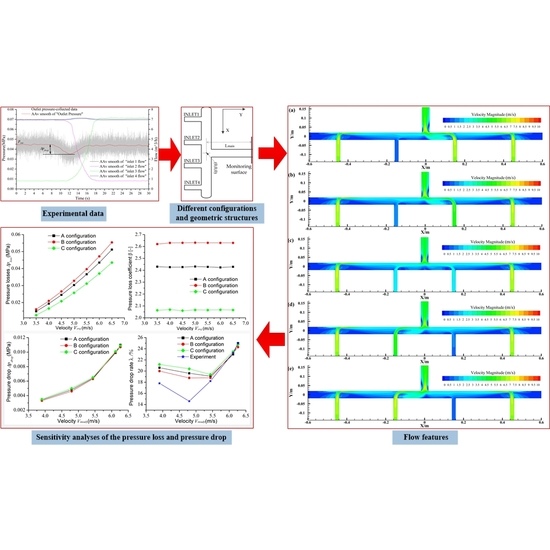
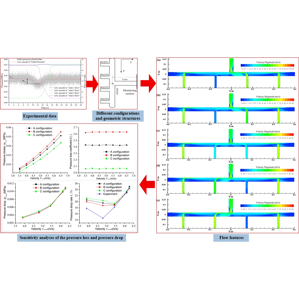
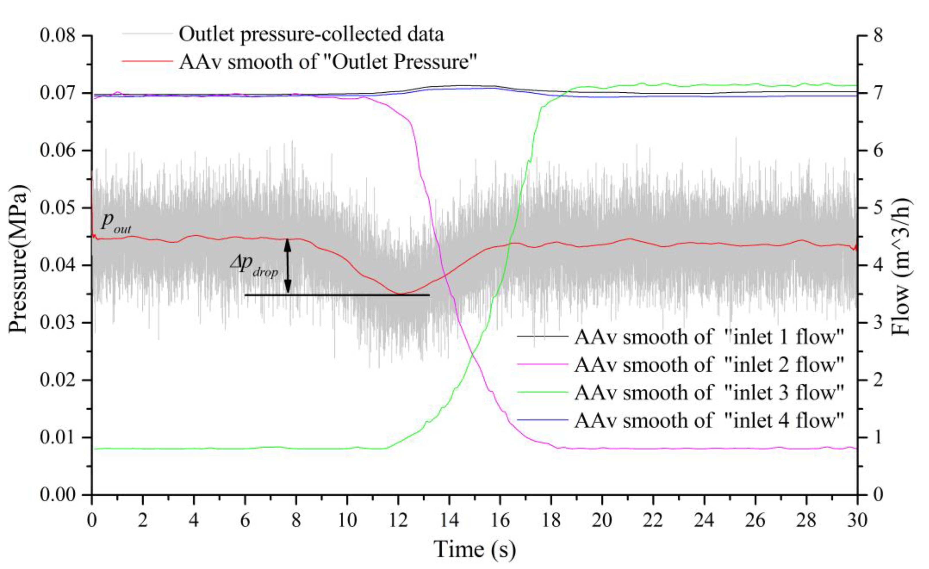
2.2. Experimental Data

In the present study, the pressure loss and pressure drop needed to be obtained from the test setup under different conditions. Pressure loss was an indirect measure because two independent pressure transducers were applied. The two transducers were located at point B in the channel pipe and point C in the main pipe. The pressure drop was measured by an independent pressure transducer located at point C in the main pipe. The inlet velocity of the channel could be calculated based on the data measured by the flowmeter located at point A in the channel pipe. The tests were performed at the channel pipe velocity ranging from 3.5 m/s to 6.5 m/s obtained by ranging the motor frequency from 29.2 Hz to 50 Hz. The Reynolds number based on the hydraulic diameter (d = 0.02 m) ranged from 77,317 to 143,568. The pressure and flowmeter transducer signals are collected using a DAQ card and processed by the LabVIEW program. Then, the data collected are processed by adjacent-averaging (AAv). To reduce measurement errors and improve the reliability of test results, all the experiments were performed three times and the average values were calculated. A set of data similar to the averages in these three sets of data was found for the simulation. Figure 3 shows the data measured for a typical, two-channel synchronous switching process under three-channel parallel operation. The flow at the inlet can be used as a boundary condition for the simulation model by the “profile” function of the ANSYS Fluent 17.0 software.

3. Geometries and Numerical Solutions

In this section, the geometric structure of the MCCS is described, based on the engineering application. In what follows, the governing equations for continuity, momentum and transport are described and solved given the boundary conditions. Finally, the simulation model is verified by experimentation.

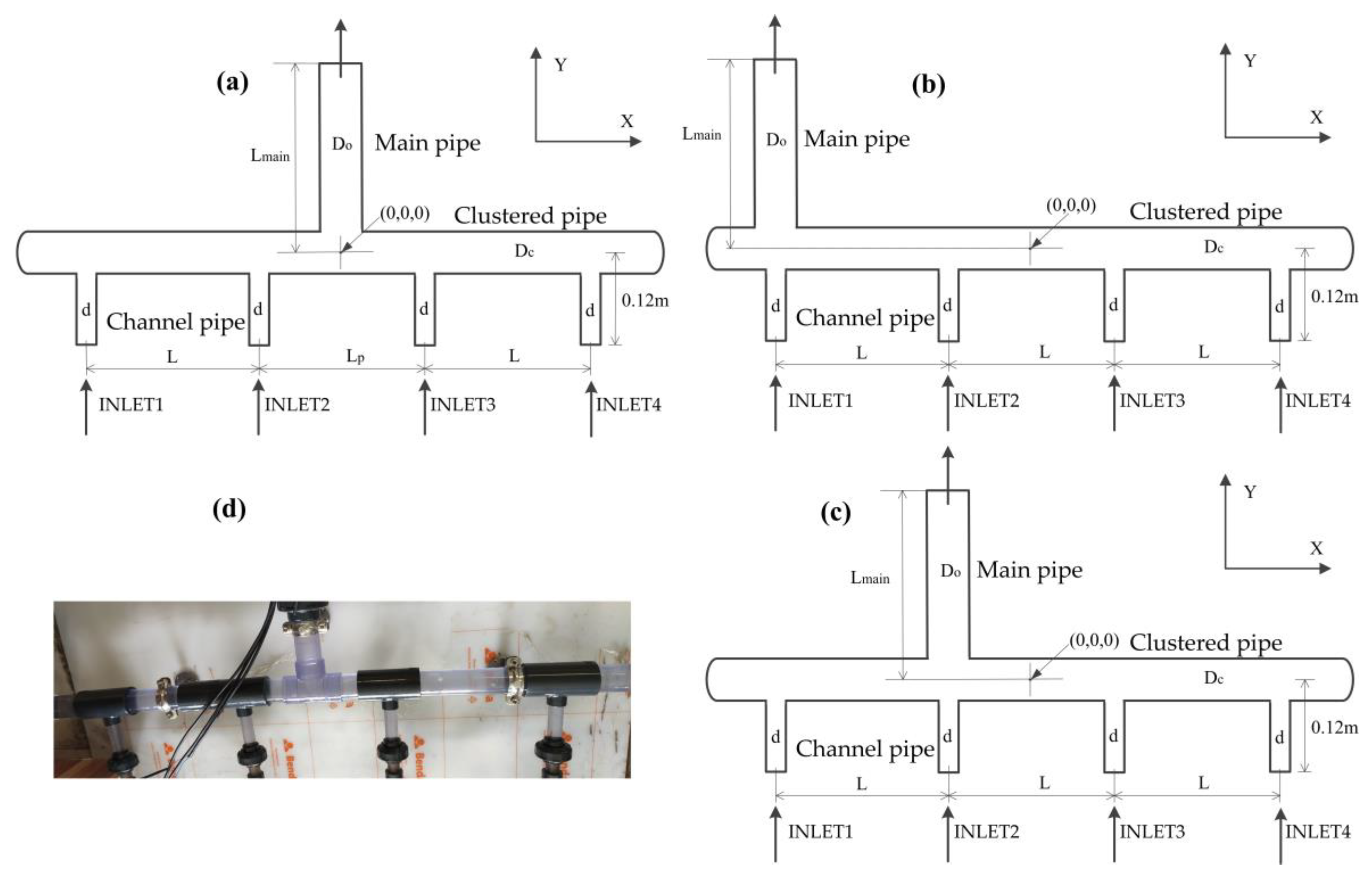
3.1. Geometries’ Structures

The MCCS structure is a combined manifold consisting of several channel pipes, a clustered pipe and a main pipe. According to reference [7], a pugged tee junction creates less pressure loss than a sharp 90 degree elbow in a turbulent flow field. Therefore, the form of the channel pipe and clustered pipe is a T-connection. It is known that the increase of water is gradually reduced rather than exponentially increased as the number of parallel pumps increases. Therefore, the number of channel pipes was initially set to four. In this paper, three different geometric structures are considered, as shown in Figure 4. Initially, the structure of configuration “A” was chosen, due to it being more common in industrial applications and simple to manufacture. The detailed size of configuration “A” and its modified versions (with the main pipe at the center of the clustered pipe) are presented in

Table 2. Design details of configuration “A”.

Configuration “A”	Dc /mm	Do /mm	Lp /mm	L /mm	Configuration “A”	Dc /mm	Do /mm	Lp /mm	L /mm
A1	40	40	300	300	A9	40	40	400	300
A2	50	40	300	300	A10	40	40	200	300
A3	60	40	300	300	A11	40	40	100	300
A4	80	30	300	300	A12	40	40	60	300
A5	80	40	300	300	A13	40	40	400	400
A6	80	50	300	300	A14	40	40	200	200
A7	80	60	300	300	A15	40	40	100	100
A8	80	80	300	300	A16	40	40	60	60

. The detailed configuration was reformed by varying the diameters of the clustered pipe, the diameters of main pipe and the distance between channel pipes.

The configurations “B” and “C” were obtained by moving the location of the main pipe compared to the configuration “A” The distances between the channel pipes were equal in configurations “B” and “C” Besides, the other details of configurations “B” and “C” are also considered in

Table 3. Design details of configurations “B” and “C”.

Configuration “B”	Dc /mm	Do /mm	L /mm	Configuration “C”	Dc /mm	Do /mm	L /mm
B1	40	40	300	C1	40	40	300
B2	50	40	300	C2	50	40	300
B3	60	40	300	C3	60	40	300
B4	80	30	300	C4	80	30	300
B5	80	40	300	C5	80	40	300
B6	80	50	300	C6	80	50	300
B7	80	60	300	C7	80	60	300
B8	80	80	300	C8	80	80	300
B9	40	40	400	C9	40	40	400
B10	40	40	200	C10	40	40	200
B11	40	40	100	C11	40	40	100
B12	40	40	60	C12	40	40	60

.

3.2. Governing Equations

The continuity equation and the momentum conservation equation are written as [22]:

$$\frac{\partial \rho }{\partial t}+\frac{\partial \left(\rho u_j\right)}{\partial x_j}=0,$$

(1)

$$\frac{\partial \left(\rho u_i\right)}{\partial t}+\frac{\partial \left(\rho u_i{u}_j\right)}{\partial x_j}=-\frac{\partial p}{\partial x_i}+\frac{\partial }{\partial x_j}\left(\mu \frac{\partial u_i}{\partial x_j}\right).$$

(2)

The modelled transport equations for k and ε in the realizable k-ε model can be expressed as follows [23]:

$$\frac{\partial \left(\rho k\right)}{\partial t}+\frac{\partial \left(\rho k{u}_j\right)}{\partial x_j}=\frac{\partial }{\partial x_j}\left[\left(\mu +\frac{{\mu }_t}{{\sigma }_k}\right)\frac{\partial k}{\partial x_j}\right]+G_k-\rho \epsilon +S_k,$$

(3)

$$\frac{\partial \left(\rho \epsilon \right)}{\partial t}+\frac{\partial \left(\rho \epsilon u_j\right)}{\partial x_j}=\frac{\partial }{\partial x_j}\left[\left(\mu +\frac{{\mu }_t}{{\sigma }_{\epsilon }}\right)\frac{\partial \epsilon }{\partial x_j}\right]+\rho C_{1}S\epsilon -\rho C_2\frac{{\epsilon }^2}{k+\sqrt{v\epsilon }}+S_{\epsilon },$$

(4)

where

$$C_1=\max \left[0.43,\frac{\eta }{\mu +5}\right],\eta =S\frac{k}{\epsilon },S=\sqrt{2S_{ij}{S}_{ij}},{\mu }_t=\rho C_{\mu }\frac{k^2}{\epsilon },S_{ij}=\frac{1}{2}\left(\frac{\partial u_j}{\partial x_i}+\frac{\partial u_i}{\partial x_j}\right).$$

(5)

In the realizable k-ε model, C_μ is no longer constant, which is given in Equation (5). Besides, the details of other parameters, such as S_k, and S_ε, are referred to in reference [8,24].

$$C_{\mu }=\frac{1}{4.04+\sqrt{6}\frac{k\sqrt{S_{ij}{S}_{ij}+{\left({\mathsf{\Omega }}_{ij}-3{\epsilon }_{ijk}{\omega }_k\right)}^2}}{\epsilon }\cos \varphi },$$

(6)

where

$$\varphi =\frac{1}{3}{\cos }^{-1}\left(\sqrt{6}\frac{S_{ij}{S}_{jk}{S}_{ki}}{{\left(S_{ij}{S}_{ij}\right)}^{3/2}}\right).$$

(7)

3.3. Simulation Details

In this article, room temperature water is used as the fluid in the simulation. The simulation model is based on the following assumptions. First, the working fluid (water) is considered a Newtonian fluid. Second, it is considered to be single-phase flow because of the neglect of air inside the pipe. Third, it is considered to be incompressible flow because of the neglect of density change. Fourth, heat transfer is not considered.

3.4. Solution Method

For the boundary conditions, at the inlet and outlet, velocity-inlet and pressure-out are set, respectively. The hydraulic diameter and turbulence intensity at the outlet and inlet are prescribed for the model. The internal pipe diameters are used for the hydraulic diameter regardless of inlet and outlet, while the turbulence intensity is set to 5%. The no slip wall was chosen for the pipe wall and the value of the roughness height of the pipe wall was set to 0.0005 m. The realizable k-ε model and standard wall functions were chosen because of the high accuracy of backflow and rotation in simulation. The governing equations are solved for steady and transient state conditions using commercial software ANSYS Fluent (Fluent 17.0, ANSYS, Pittsburgh, PA, USA). The SIMPLEC algorithm is used to couple the pressure and velocity fields. Moreover, the second-order, upwind, discrete scheme was adopted to satisfy the requirements for precision and steady state. Finally, the residuals were set to 1 × 10⁻⁴ to obtain relatively accurate solutions.

In particular, it is necessary to expand the computational domain of the simulation analysis to obtain the pressure drop under switching conditions, as shown in Figure 5. The extended section simulates the load, so that the numerical simulation has the same resistance as the actual resistance. The pressure drop caused by two-channel synchronous switching is obtained on the monitoring surface by transient analysis, using the experimental data as the velocity-inlet, and the atmospheric pressure as the pressure-outlet.

3.5. Grid Independence

To obtain a highly efficient grid for use in the simulations, the steps were as follows. First, base geometry discretization was performed with ANSYS Meshing. The tetrahedral elements and hexahedral elements were used in the computational mesh. The y+ for the mesh was set to approximately 30; the maximum number of inflation layers was set to 6; and the growth rate was set to 1.2. Second, in order to establish grid independence and validate the model, the experimental and simulated fluids were compared in terms of the total pressure loss for models with different meshes, as shown in

Table 4. Mesh sensitivity analysis for configuration “A1”.

Relevance	Refined Size	Grid Number	△ploss.sim	△ploss.exp	SE/%
100	1.5 mm	2,482,014	0.0392	0.0429	8.6247
100	1.8 mm	1,656,966	0.0404	0.0429	5.8275
100	2 mm	1,329,794	0.0400	0.0429	6.7599
50	2 mm	1,214,846	0.0398	0.0429	7.2261
35	2 mm	1,169,411	0.0390	0.0429	9.0909
0	2 mm	1,093,832	0.0387	0.0429	9.7902
0	3 mm	465,797	0.0371	0.0429	13.5198
100	/	535,951	0.0372	0.0429	13.2867
50	/	384,365	0.0376	0.0429	12.3543

. The different grids are employed by the change of the “relevance” parameter and the size of the refined mesh at the junction. Since one of the most important purposes of the study is to investigate the total pressure loss of the MCCS, the evaluation criteria for grid independence and model validation are based on the SE value in the simulation results with different meshes and the experiments. The results for configuration “A1” are shown in Table 4. It can be seen that as the number of mesh elements increases, the results do not change significantly. Similarly, the grid cells’ change test was performed for configurations “B” “C” and the other modified designs. Therefore, the mesh with the relevance center of 100 and refined size of 2 mm was accepted. Meanwhile, the present CFD modelwais able to predict the total pressure loss within an 8% deviation from the simulations and experimental measurements. Thus, the simulation model was proven feasible.

The total pressure loss differences (SE) with different meshes are calculated with Equation (10) under the same boundary conditions.

$$p_{in}=\left(p_1+p_2+\cdots +p_n\right)/n,$$

(8)

$$\Delta p_{loss}=p_{in}-p_{out},$$

(9)

$$SE=\frac{\Delta p_{loss.\exp }-\Delta p_{loss.\mathrm{sim}}}{\Delta p_{loss.\exp }}\times 100\%.$$

(10)

3.6. Model Validation

Experimental tests of the test section pressure and flow were investigated, which made it possible to validate the simulation model built by ANSYS Fluent (Fluent 17.0, ANSYS, Pittsburgh, PA, USA). The present Fluent model was validated based on pressure loss and pressure drop. The details of the test conditions were set to an inlet velocity ranging from 3.5 m/s to 6.5 m/s and different numbers of channel pipes. Additionally, the switching time of the two-channel synchronous switching process under three-channel parallel operation was set to 10 s. The pressure loss of the structure itself from the experiment and the simulation are shown in Figure 6a. The pressure drop caused by synchronous switching is presented in Figure 6b. The simulation results present an increasing trend of pressure loss and pressure drop with the inlet velocity, which are slightly different from the trends of the experimental results. Nevertheless, the deviation of pressure loss was smaller than 12%; the deviation of pressure drop decreased from 31 to 2% with increasing velocity; and the experimental and numerical trends were consistent. Thus, the simulation model was reliably validated and was used for analysis of pressure loss, pressure drop and flow features, as described in the following sections.

4. Results and Discussion

It was the objective of this paper to study the energy losses of the MCCS structure in water supply. The energy loss mainly depends on the pressure loss of the structure itself and the pressure drop caused by different working conditions. In this paper, the reason for the pressure drop is a two-channel synchronous switching process in a three-channel parallel operation. Furthermore, the influence of certain MCCS structure parameters and other parameters that affect the energy loss were investigated by simulation. In particular, the inlet velocity (i.e., the inlet flow) of the switching channel during transient analysis was obtained in experiments (see Figure 3). More specifically, in order to analyze the causes of pressure loss and pressure drop, the major flow features of the MCCS structure were investigated using the mean velocity contours in the simulation model.

4.1. The Influence of Clustered Pipe Diameter

An influence of clustered pipe diameter on the pressure loss and pressure drop was investigated by simulation. The results are presented in Figure 7 in the form: pressure loss or pressure drop as a function of clustered pipe diameter Dc/d.

The influence of clustered pipe diameter on pressure loss for all configurations was investigated by increasing the clustered pipe diameter from 40 to 80 mm while the rest of the considered variables remained constant. The inlet velocity was set to 6 m/s and the diameter of the channel pipe (d) was set to 20 mm; meanwhile, the Dc/d changed from 2 to 4. Operation with four parallel channels was considered representative for further investigations. It can be observed from Figure 7a that the total pressure loss for all configurations decreases gradually with increasing clustered pipe diameter; tends to stabilize; and then, increases slightly. According to [25], total pressure loss is composed of friction loss and local loss. The friction loss mainly depends on the friction factor, which is basically unchanged for the same clustered pipe configuration. The flow space at the intersection of the channel pipe and the clustered pipe increases with the increasing of the diameter of clustered pipe for the same configuration. This leads to a reduction in local loss caused by a change in the velocity direction. When the diameter of the clustered pipe increases to a certain extent, such as in configuration “A” the flow of water entering the clustered pipe is the entering jet, and the biggest change in the velocity gradient is not the wall of clustered pipe, and there is no sharp change in the velocity direction, as shown in Figure 8. This leads to almost no big change in local loss, and the change in total pressure loss is determined by the friction loss; that is, the total pressure loss increases slightly in a stable condition based on the Darcy formula.

The total pressure loss for configuration “A” is always larger than for “C” Velocity contours for the configurations “A” and “C” (see Figure 9) can explain this phenomenon. Compared with configuration “A” the location of the main pipe is altered in configuration “C” so that the main pipe and channel pipe are placed in inline. This causes a reduction in local loss caused by a sharp change in the velocity direction.

What is interesting in Figure 7a is the abnormal change in pressure loss for configuration “B” The total pressure loss of configuration “B” is greater than configuration “A” when Dc/d = 2, but tends toward configuration “C” at Dc/d > 2.5. This is due to the dominating influence of local losses over total pressure loss when Dc/d = 2. However, the friction loss plays a major role in total pressure loss when Dc/d = 4.

The influence of clustered pipe diameter on pressure drop was investigated by increasing the clustered pipe diameter from 40 to 80 mm (that is, Dc/d obtained changes from 2 to 4). The time of the switching was set to 10 s. The inlet velocity boundary conditions of the switching channel can be obtained in experiment and then used in transient analysis with the “profile” function. It can be seen from Figure 7b that the pressure drop for all configurations decreased gradually with increasing clustered pipe diameter, and tended to stabilize. The curves for different configurations were almost the same; that is, different configurations are not sensitive to the effects of pressure drop. To illustrate the cause of the pressure drop, flow features were investigated using the mean velocity contours in the simulation model. Considering configuration “A” of Dc/d = 2 as an example, the predicted flow fields during the switching process are shown in Figure 10. It can be observed that the velocity contours at the main pipe changes dramatically, and lead to a pressure drop at the main pipe. The velocity is well distributed in each channel pipe, but the flow patterns are poor and asymmetrical in the clustered pipe, especially in the region between X = −0.16 m and X = 0.16 m. The velocity contours near the channel pipe, which is not involved in switching, do not change much during the switching process.

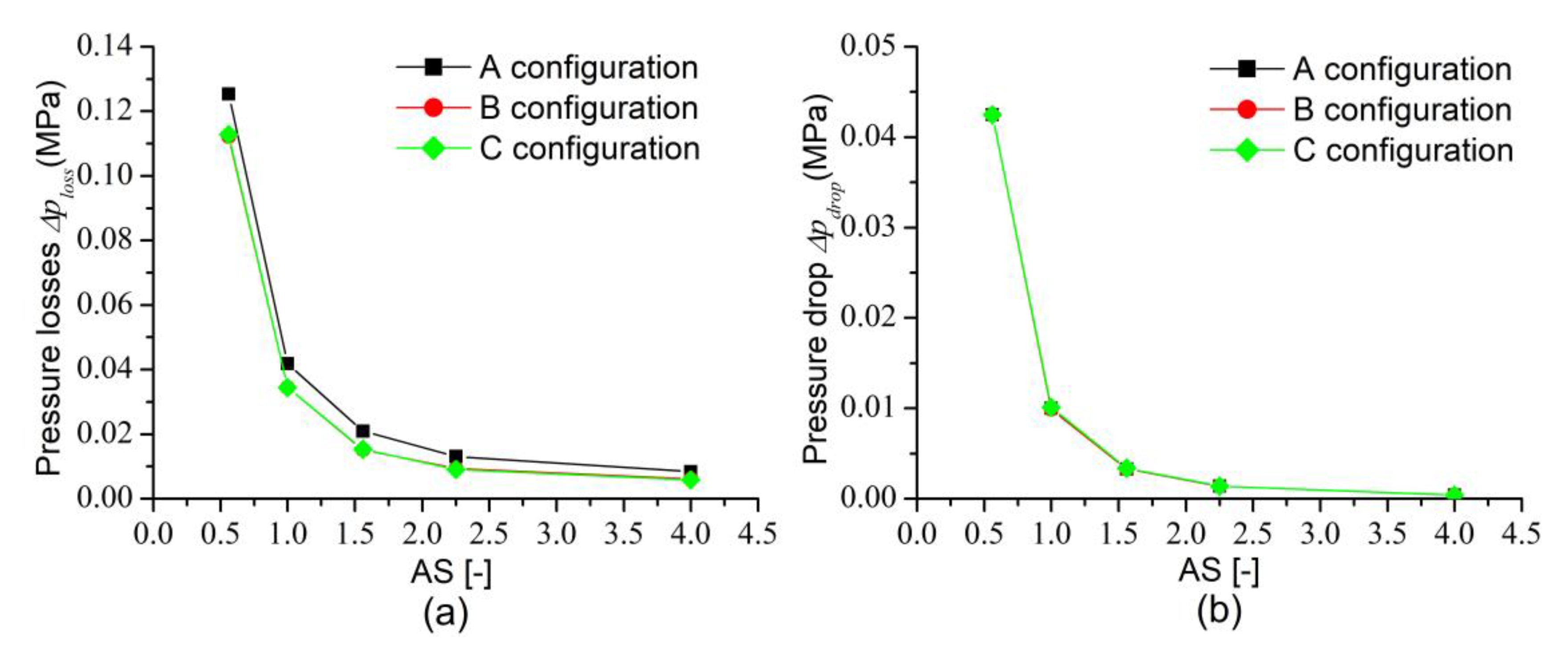
4.2. The Influence of Main Pipe Diameter

To analyze the influence of the main pipe diameter on pressure loss and pressure drop, the main pipe diameter was changed from 30 to 80 mm while maintaining other parameters. The clustered pipe diameter was set to 80 mm, the channel pipe diameter (d) was set to 20 mm and the pitch between channels was kept at 300 mm. The dimensionless parameter AS (D_o²/(4 × d²)) was used at this point, which represents the ratio of the cross-sectional area of the main pipe to the total cross-sectional area of the channel pipes. The results are presented in Figure 11 in the forms: pressure loss and pressure drop as functions of cross-sectional area ratio AS.

Figure 11a shows a comparison of the total pressure loss for configurations “A” “B” and “C” for different main pipe diameters. Total pressure loss is always significantly greater for “A” configuration than for the configurations “B” and “C” It was noticed that the total pressure loss for all configurations decreases with increasing main pipe diameter. However, it is different for the gradient of total pressure loss reduction in different ranges. Notably, the total pressure loss changes sharply when AS < 1. It is known that the diameter of the outlet pipe is inversely proportional to velocity based on the continuity equation. The argument is further proven in Figure 12. This leads to the reduction of total pressure loss with increasing AS. Furthermore, the friction loss is not only related to velocity, but also inversely proportional to the pipe diameter. Thus, the gradient of total pressure loss changes more greatly when AS < 1 than when AS > 1.

Figure 11b shows a comparison of the pressure drop for configurations “A” “B” and “C” with different main pipe diameters. Pressure drops are inversely proportional to the main pipe diameter. Furthermore, the results show that a change in pressure drop is negligible for the different configurations. According to the mathematical analysis and simulation calculations, it can be concluded that the pressure of outlet increases with increasing AS (diameter of main pipe). Therefore, it is necessary to evaluate the variation of the pressure drop value from another dimension; that is, the ratio of pressure drop to outlet pressure. The percentages of pressure drop to outlet pressure for different AS values are presented in

Table 5. Percentage of pressure drop to outlet pressure for different AS values.

AS	0.5625	1	1.56	2.25	4
△pdrop/pout	21.8%	22.8%	23.6%	25.9%	36%

. The presented values show that the magnitude of the decrease in outlet pressure is reduced, but the ratio of the outlet pressure is increased with increasing the diameter of main pipe.

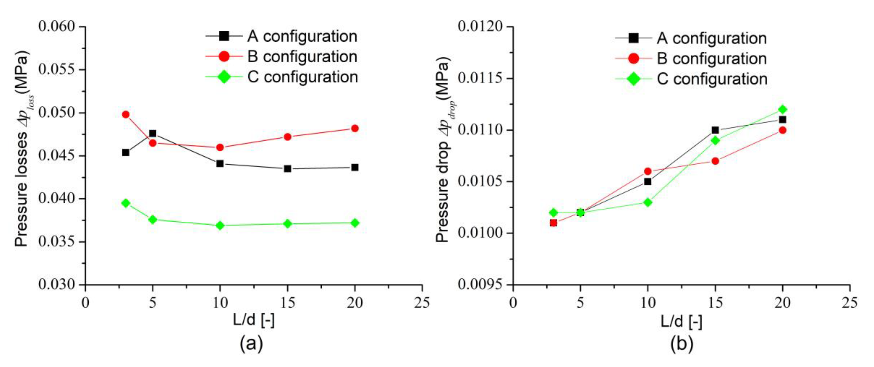
4.3. The Influence of Pitch

The pitches between channels were set to 60, 100, 200, 300 and 400 mm, respectively, while the channel pipe diameter (d) was set to 20 mm. The clustered pipe diameter was set to 40 mm and the main pipe diameter was set to 40 mm. Besides, by varying the configuration, corresponding curves of pressure loss and pressure drop were obtained, as shown in Figure 13a,b respectively. The results are presented in a form: pressure loss or pressure drop as a function of L/d.

A comparison of the total pressure losses for configurations “A” “B” and “C” for different channel pitches was investigated by simulation. As it is illustrated in Figure 13a, the total pressure loss for configurations “B” and “C” first decreased with a large gradient, and then increased with a small gradient with increasing pitch of the channel, and configuration “A” increases first and then decreases. It was noticed that when L was more than 10d, the total pressure loss rankings from high to low were “B” configuration, “A” configuration and “C” configuration. That is because the friction loss plays a major role with increasing pitch of channels. We know that the paths of water flow from the inlet to the outlet for configurations “A” “B” and “C” were 4L, 6L and 4L, respectively. At the same time, in the preceding paragraphs, it was discerned that the arrangement of the “C” configuration is smaller than the “A” configuration for local loss. It was also seen that when the L is less than 10d, the law of the total pressure loss for configurations “A” “B” and “C” is weakly applicable. This is due to the water flow in different channels pipes effecting each other when the pitch is small. From Figure 14, it can be observed that the number of vortex structures decreases with increasing the channel pitch. This means that local losses caused by the change of velocity direction decrease with increasing channel pitch.

In case of the pitch between channels is non-equidistant, the variation of total pressure loss is shown in

Table 6. Influence of non-equidistant channels for configuration “A”.

Lp/d	3	5	10	15	20
△ploss/MPa	0.0426	0.0486	0.0442	0.0435	0.0436
△pdrop/MPa	0.0104	0.0103	0.011	0.011	0.0111

. Take the example of configuration “A” the pitch Lp changes from 3d to 20d while maintaining other parameters. The results shown that the change of the total pressure loss maintains the same trend compared to the equal pitch configuration.

A comparison of the pressure drop for configurations “A” “B” and “C” for different channel pitches was investigated, as shown in Figure 13b. The pressure drop for all configurations increases gradually with increasing channel pitch. The curves for different configurations are almost the same, that is, different configurations are not sensitive to the effects of pressure drop.

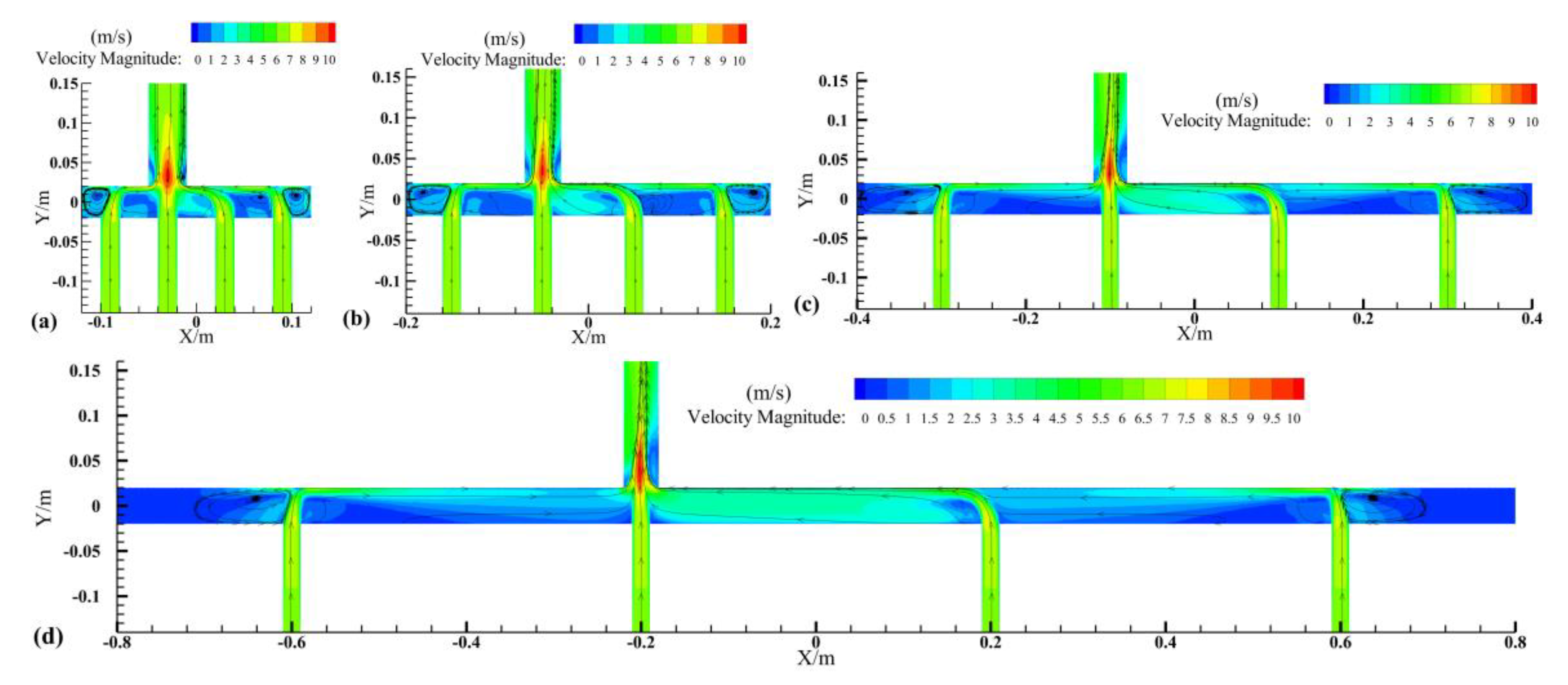
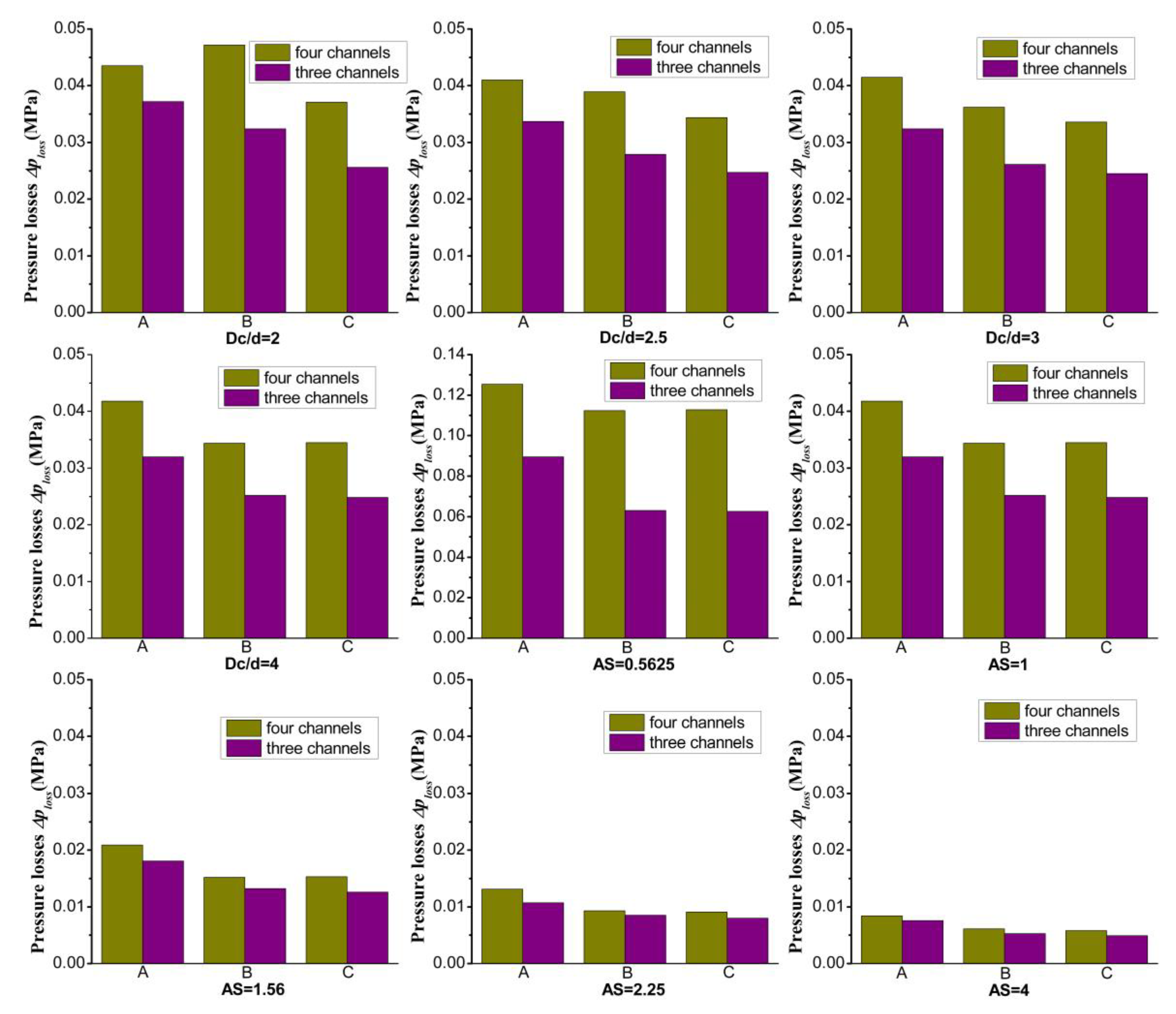
4.4. The Influence of the Number of Channels

The channel pipe diameter was set to 20 mm, the pitch between channels was set to 300 mm, and the inlet velocity was set to 6 m/s. The numbers of channels were set to four and three respectively. By varying the clustered pipe diameter and the main pipe diameter, a histogram of the relationships among configurations “A” “B” and “C” with different numbers of channels, were obtained, as shown in Figure 15.

The histogram of total pressure loss obtained with different number of channels all show a similar trend: that the loss with four channels is greater than with three channels. It is also can be seen that the influences of different geometric parameters on the total pressure loss are the same. However, there is a special case that the total pressure loss for the configuration “B” is the biggest with four-channel operation at Dc/d = 2. In this paper, the switching conditions require three channels of supply and one channel for standby. Therefore, it is necessary to consider the difference of total pressure loss caused by different channel combinations. The total pressure loss of configurations “A” “B” and “C” with different channel combination under three parallel channel operation are presented in

Table 7. Pressure losses of “A” “B” and “C” configurations with different channel combinations under three parallel channel operations.

Configuration	“A”		“B”				“C”
Channel	123/234	124/134	123	124	134	234	123	124	134	234
△ploss/MPa	0.0372	0.0365	0.0324	0.0326	0.034	0.0507	0.0256	0.0257	0.0372	0.0324

. The values presented show that smaller pressure loss occurs when the inlet channel and outlet pipe are in line. On the contrary, the total pressure loss is large when the distance between inlet channels and the outlet pipe is long. For example, the total pressure loss of the channel 234 combination of configuration “B” is 49.5% bigger than the channel 123 combination of configuration “C” This suggests that the combination of different channels should be fully considered.

4.5. The Influence of Inlet Velocity

The influence of inlet velocity for the total pressure loss was investigated by increasing the inlet velocity from 3.5 m/s to 6.5 m/s for all configurations. The influence of inlet stability velocity for the pressure drop was investigated by increasing the motor frequency from 29.2 Hz to 50 Hz for all configurations. Besides, the parameters of Dc/d, AS and L were set to 2, 1 and 300 mm, respectively. The results are shown in the Figure 16 and Figure 17, respectively.

To analyze the results more intuitively and accurately, the data of the simulation are expressed in dimensional and dimensionless forms. The energy losses of the MCCS structure presented in a dimensionless form are expressed as the pressure loss coefficient and pressure drop rate.

Pressure loss coefficient β and pressure drop rate λ are defined by the following Equations:

$$\beta =\frac{2\cdot \Delta p_{loss}}{\rho \cdot v_{avg}^2},$$

(11)

$$\lambda =\frac{\Delta p_{drop}}{p_{out}}.$$

(12)

It can be seen in Figure 16a that the total pressure loss for all configurations increases with increasing inlet velocity. This is considered to be the result when the channel flow collides directly with the wall of the clustered pipe resulting in a great loss of the energy. And the larger the inlet velocity is, the greater the total pressure loss is. Furthermore, the order of the total pressure loss from high to low is configuration “B” “A” and “C” due to the influence of the structure. The analyses done in Figure 16b show that for a typical inlet velocity, the change in pressure loss coefficient is negligible. However, it is obvious that the configuration “C” has the least impact on total pressure loss.

It can be seen in Figure 17a that the pressure drop increases as the inlet stability velocity goes from 3.5 m/s to 6.5 m/s, for all the configurations considered. Furthermore, the influence of the configuration is mixed with the effect of the velocity; it is not possible to define a clear influence of the configuration. Therefore, the pressure drop rate was introduced to analyze the pressure drop, as shown in Figure 17b. From the images above, it is evident that there exists one extreme point, denoted at 5.5 m/s. When the inlet stability velocity is less than 5.5 m/s, the arrangement of configuration “B” is optimal rather than configurations “A” and “C” When the inlet stability velocity is greater than 5.5 m/s, the influence of the arrangement of the configuration on the pressure drop is negligible. A similar conclusion is obtained by analyzing the experimental results, as shown in Figure 17b. This suggests that a decrease in the inlet velocity has more influence on the decrease in energy loss.

5. Conclusions

In this paper, the performance of the MCCS structure was investigated numerically to analyze the influence of its geometric parameters on the pressure loss of the structure itself and the pressure drop caused by synchronous switching. The results show that:

• The configuration “C” can be considered a costless method of decreasing total pressure loss in a multi-channel, confluent supply structure. For pressure drop, different configurations are insensitive to their effects.
• An increase of clustered pipe diameter results in the pressure loss decreasing sharply first, and then increasing slightly. Increasing the pitch between channels can result in the same trend of pressure loss. For pressure drop, it is decreased with increasing clustered pipe diameter, but the trend is the opposite for channel pitch.
• Increasing the main pipe diameter will reduce the pressure loss and the pressure drop. The gradient of change in AS < 1 is significantly larger than in AS > 1. However, in engineering applications, the main pipe diameter cannot be increased without limits. According to the evaluation criteria of the pressure drop rate, the ratio of the pressure drop to the outlet pressure increases with increasing main pipe diameter, which is unfavorable to energy savings.
• It was found that the pressure loss of four channels is greater than three channels. However, the combination of different channels should be fully considered in switching conditions. That is, the main pipe and channel pipe should be placed in inline in order to reduce the pressure loss.

The results presented in this work can help with designing a multi-channel, confluent supply geometrical structure from an energy-efficiency standpoint. In addition, for the operator, a suitable velocity (flow rate) can further reduce energy loss. It should be stated that the conclusions from the case study are from numerical simulations reflecting ideal scenarios. In practical applications, different pipe materials and the differences in processing technology may cause more or less pressure changes. Nevertheless, the numerical simulations’ analysis expresses the correct trends of pressure drop and pressure loss. In this research, the switching of two channels is assumed to be synchronous. This is due to the pressure drop being relatively large during synchronous switching, and it is more intuitive when comparing the influence laws of different geometric factors. Of course, the next step of this research will be to analyze the variation of pressure drop under different influencing factors (non-structural geometric factors).

References

1. Viholainen, J.; Tamminen, J.; Ahonen, T.; Ahola, J.; Vakkilainen, E.; Soukka, R. Energy-efficient control strategy for variable speed-driven parallel pumping systems. Energy Effic. 2013, 6, 495–509. [Google Scholar] [CrossRef]
2. Wu, P.; Lai, Z.; Wu, D.; Wang, L. Optimization Research of Parallel Pump System for Improving Energy Efficiency. J. Water Resour. Plan. Manag. 2014, 141, 1–8. [Google Scholar] [CrossRef]
3. Rezghi, A.; Riasi, A. The interaction effect of hydraulic transient conditions of two parallel pump-turbine units in a pumped-storage power plant with considering “S-shaped” instability region: Numerical simulation. Renew. Energy 2018, 118, 896–908. [Google Scholar] [CrossRef]
4. Rezghi, A.; Riasi, A. Sensitivity analysis of transient flow of two parallel pump-turbines operating at runaway. Renew. Energy 2016, 86, 611–622. [Google Scholar] [CrossRef]
5. Wan, W.; Li, F. Sensitivity Analysis of Operational Time Differences for a Pump–Valve System on a Water Hammer Response. J. Press. Vessel Technol. 2015, 138, 011303. [Google Scholar] [CrossRef]
6. Arun Shankar, V.K.; Umashankar, S.; Paramasivam, S.; Hanigovszki, N. A comprehensive review on energy efficiency enhancement initiatives in centrifugal pumping system. Appl. Energy 2016, 181, 495–513. [Google Scholar] [CrossRef]
7. Bluestein, A.M.; Helenbrook, B.T.; Venters, R.; Ahmadi, G.; Bohl, D. Turbulent Flow Through a Ducted Elbow and Plugged Tee Geometry: An Experimental and Numerical Study. J. Fluids Eng. 2019, 141, 081101. [Google Scholar] [CrossRef]
8. Gandhi, M.S.; Ganguli, A.A.; Joshi, J.B.; Vijayan, P.K. CFD simulation for steam distribution in header and tube assemblies. Chem. Eng. Res. Des. 2012, 90, 487–506. [Google Scholar] [CrossRef]
9. Liu, H.; Li, P.; Wang, K. The flow downstream of a bifurcation of a flow channel for uniform flow distribution via cascade flow channel bifurcations. Appl. Therm. Eng. 2015, 81, 114–127. [Google Scholar] [CrossRef]
10. Amanowicz, Ł. Influence of geometrical parameters on the flow characteristics of multi-pipe earth-to-air heat exchangers—Experimental and CFD investigations Łukasz. Appl. Energy 2018, 226, 34. [Google Scholar] [CrossRef]
11. Zhou, J.; Sun, Z.; Ding, M.; Bian, H.; Zhang, N.; Meng, Z. CFD simulation for flow distribution in manifolds of central-type compact parallel flow heat exchangers. Appl. Therm. Eng. 2017, 126, 670–677. [Google Scholar] [CrossRef]
12. Karvounis, P.; Koubogiannis, D.; Hontzopoulos, E.; Hatziapostolou, A. Numerical and experimental study of flow characteristics in solar collector manifolds. Energies 2019, 12, 1431. [Google Scholar] [CrossRef]
13. García-Guendulain, J.M.; Riesco-Avila, J.M.; Elizalde-Blancas, F.; Belman-Flores, J.M.; Serrano-Arellano, J. Numerical study on the effect of distribution plates in the manifolds on the flow distribution and thermal performance of a flat plate solar collector. Energies 2018, 11, 1077. [Google Scholar] [CrossRef]
14. López-López, J.C.; Salinas-Vázquez, M.; Verma, M.P.; Vicente y Rodríguez, W.; Galindo-Garcia, I.F. Computational fluid dynamic modeling to determine the resistance coefficient of a saturated steam flow in 90° elbows for high Reynolds number. J. Fluids Eng. 2019, 141, 111103. [Google Scholar] [CrossRef]
15. Zardin, B.; Cillo, G.; Rinaldini, C.A.; Mattarelli, E.; Borghi, M. Pressure losses in hydraulic manifolds. Energies 2017, 10, 310. [Google Scholar] [CrossRef]
16. Zardin, B.; Cillo, G.; Borghi, M.; D’Adamo, A.; Fontanesi, S. Pressure losses in multiple-elbow paths and in V-bends of hydraulic manifolds. Energies 2017, 10, 60788. [Google Scholar] [CrossRef]
17. Li, A.; Chen, X.; Chen, L. Numerical investigations on effects of seven drag reduction components in elbow and T-junction close-coupled pipes. Build. Serv. Eng. Res. Technol. 2015, 36, 295–310. [Google Scholar] [CrossRef]
18. Li, A.; Chen, X.; Chen, L.; Gao, R. Study on local drag reduction effects of wedge-shaped components in elbow and T-junction close-coupled pipes. Build. Simul. 2014, 7, 175–184. [Google Scholar] [CrossRef]
19. Liu, H.; Li, P. Even distribution/dividing of single-phase fluids by symmetric bifurcation of flow channels. Int. J. Heat Fluid Flow 2013, 40, 165–179. [Google Scholar] [CrossRef]
20. Rak, J.R.; Pietrucha-Urbanik, K. An approach to determine risk indices for drinking water-study investigation. Sustainability 2019, 11, 3189. [Google Scholar] [CrossRef]
21. Urbanik, M.; Tchórzewska-Cieślak, B.; Pietrucha-Urbanik, K. Analysis of the Safety of Functioning Gas Pipelines in Terms of the Occurrence of Failures. Energies 2019, 12, 3228. [Google Scholar] [CrossRef]
22. Ferziger, J.H.; Peric, M. Computational Methods for Fluid Dynamics; Sprigner: Berlin, Germany, 1999. [Google Scholar]
23. Shih, T.H.; Liou, W.W.; Shabbir, A.; Yang, Z.; Zhu, J. A new κ-ε eddy viscosity model for high reynolds number turbulent flows. Comput. Fluids 1995, 24, 227–238. [Google Scholar] [CrossRef]
24. Liu, X.; Yue, S.; Lu, L.; Gao, W.; Li, J. Experimental and numerical studies on flow and turbulence characteristics of impinging stream reactors with dynamic inlet velocity variation. Energies 2018, 11, 1717. [Google Scholar] [CrossRef] [Green Version]
25. Idelchik, I.E. Handbook of Hydraulic Resistance, 2nd ed.; Hemisphere Publishing: Washington, DC, USA, 1986. [Google Scholar]
Figure 1. Mobile application of a multi-channel confluent supply (MCCS) structure in the field of fire protection.
Energies 12 04354 g001
Figure 2. Schematic of the test setup and connections: (1) water tank; (2) hand valve; (3) frequency converter; (4) vacuum meter; (5) centrifugal pump; (6) pressure gage; (7) check valve; (8) ball valve; (9) pneumatic valve; (10) flowmeter; (11) pressure transducer; (12) electric control valve; (13) air-vent valve; (14) air compressor; (15) DAQ Card; (16) analysis recorder.
Energies 12 04354 g002
Figure 3. Measurement data for a typical operation.
Energies 12 04354 g003
Figure 4. Different schema of the structure: (a) configuration “A”; (b) configuration “B”; (c) configuration “C”; (d) physical objects of configuration “A”.
Energies 12 04354 g004
Figure 5. The computational domain of the simulation study.
Energies 12 04354 g005
Figure 6. Comparison of experimental and numerical investigations: (a) pressure loss; (b) pressure drop.
Energies 12 04354 g006
Figure 7. Influence of clustered pipe diameter on: (a) pressure loss; (b) pressure drop.
Energies 12 04354 g007
Figure 8. Velocity magnitude contours for configuration “A” cases: (a) Dc/d = 2; (b) Dc/d = 2.5; (c) Dc/d = 4.
Energies 12 04354 g008
Figure 9. Velocity magnitude contours for Dc/d = 3 cases: (a) configuration “A”; (b) configuration “C”.
Energies 12 04354 g009
Figure 10. Velocity magnitude contours at the various times: (a) 10 s; (b) 13 s; (c) 15 s; (d) 17 s; (e) 20 s.
Energies 12 04354 g010
Figure 11. Influence of main pipe diameter on: (a) pressure loss; (b) pressure drop.
Energies 12 04354 g011
Figure 12. Velocity magnitude contours for configuration “C” cases: (a) AS = 0.5625; (b) AS = 4.
Energies 12 04354 g012
Figure 13. Influence of channels pitch on: (a) pressure loss; (b) pressure drop.
Energies 12 04354 g013
Figure 14. Velocity magnitude contours for configuration “C” cases: (a) L = 3d; (b) L = 5d; (c) L = 10d; (d) L = 20d.
Energies 12 04354 g014
Figure 15. Influence of number of channels on the total pressure loss.
Energies 12 04354 g015
Figure 16. Influence of inlet velocity on the total pressure loss: (a) pressure losses; (b) pressure loss coefficient.
Energies 12 04354 g016
Figure 17. Influence of inlet stability velocity on the pressure drop: (a) pressure drop; (b) pressure drop rate.
Energies 12 04354 g017