Forecasting Oil Price Using Web-based Sentiment Analysis


Abstract
: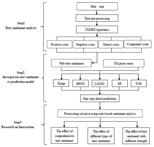
1. Introduction
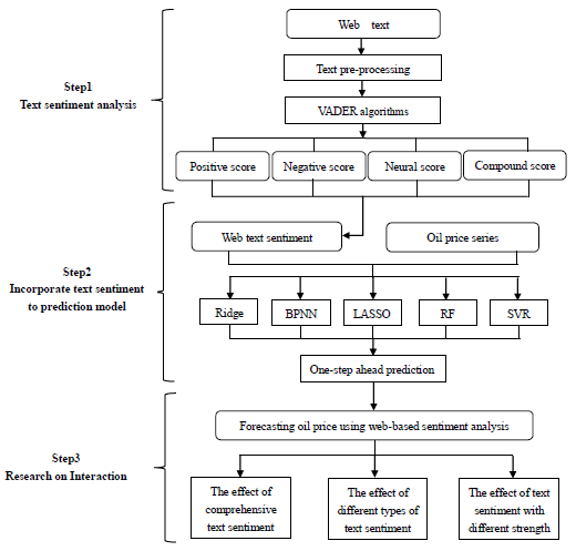
2. Materials and Methods
2.1. Web Text Pre-Processing
2.2. Web Text Sentiment
| Algorithm 1. VADER sentiment algorithms. | |
| Input: Text to be analysed, tendency rules, emotional dictionary. | |
| Output: , , , and | |
| Step 1. Calculate the emphasised weights in the sentence according to the tendency rule. | |
| Step 2. Calculate using the formula below for using Equation (1). | |
| (1) | |
| where indicates an article, indicates vocabulary, indicates vocabulary score, is a symbol function, emphasises weight, and dictionary information is used to measure vocabulary with emphasis in the article. For example, “very” and “extremely” can enlarge the value of . is a normalisation function, which is mapped onto to a real number on . | |
| Step 3. Calculate the sum scores including , , and by using Equation (2). | |
| (2) | |
| Step 4. Include the emphasis weight to get the modified sum score including , , and by using Equation (3). | |
| (3) | |
| Step 5. Calculate the total score, , using Equation (4). | |
| (4) | |
| Step 6. Calculate the final score based on the total score using Equation (5). | |
| (5) | |
2.3. Oil price Forecasting Model
3. Empirical Analysis
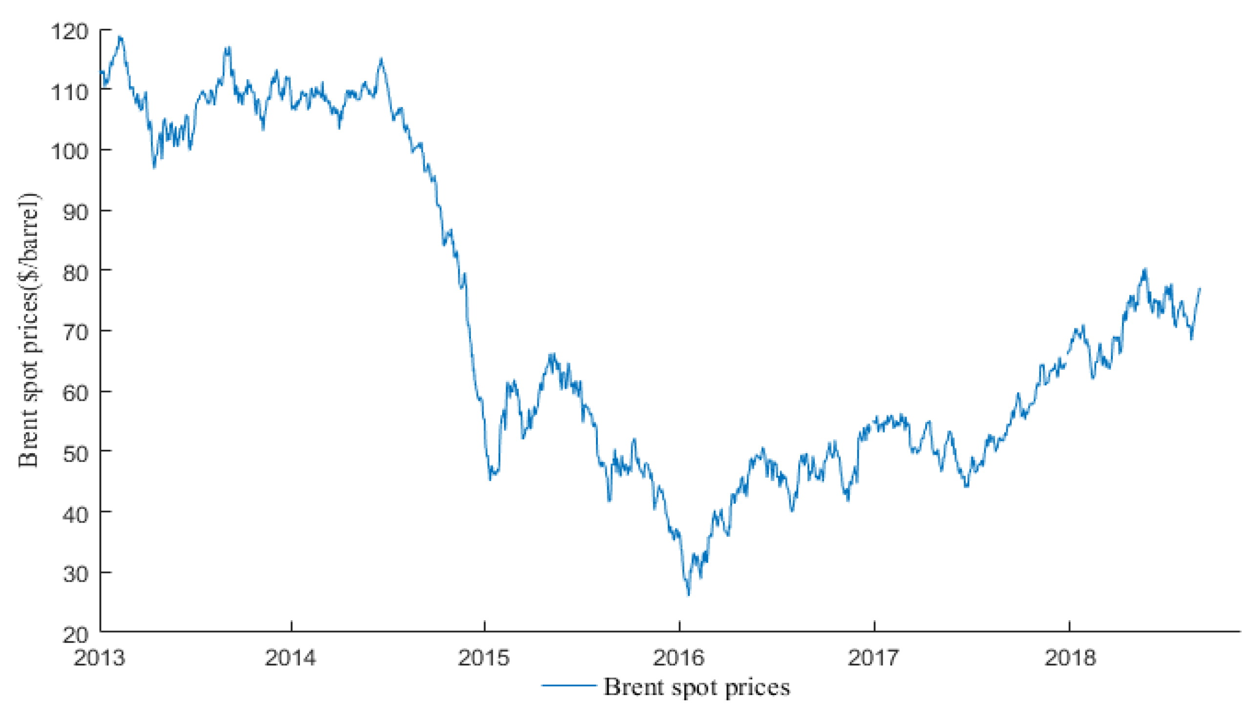
3.1. Data Sources
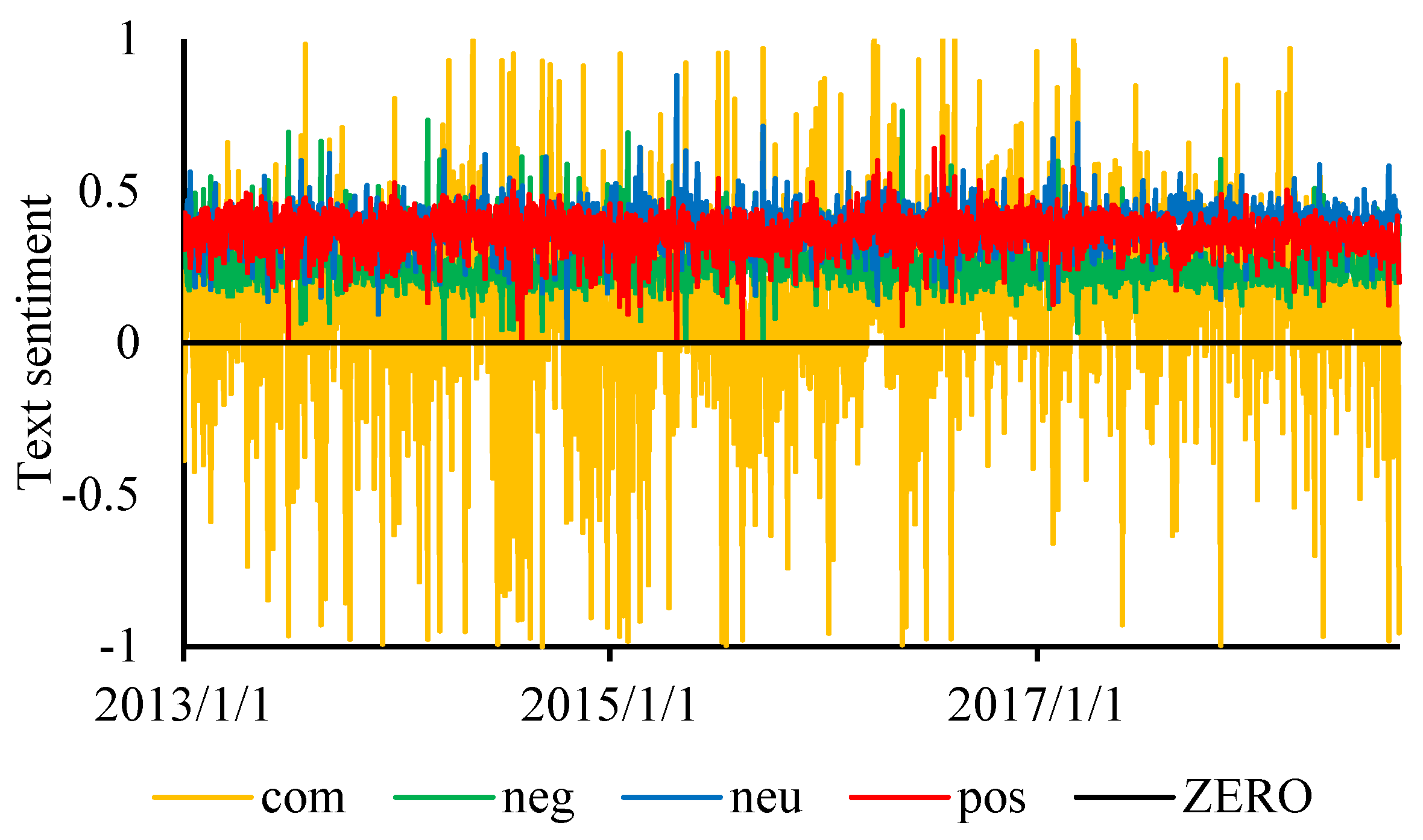
3.2. Text Sentiment Analysis
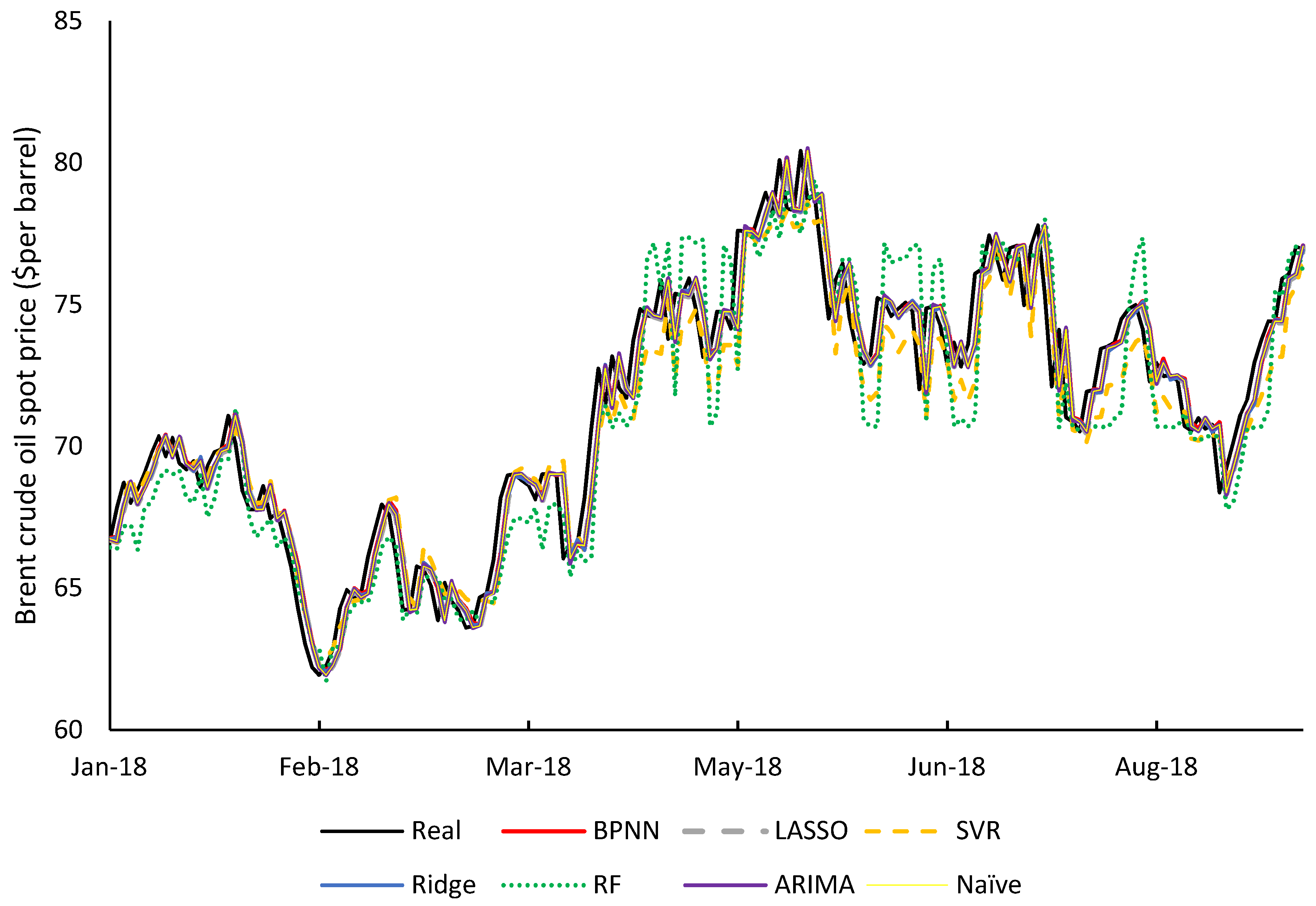
3.3. Choice of Oil Price Forecasting Model
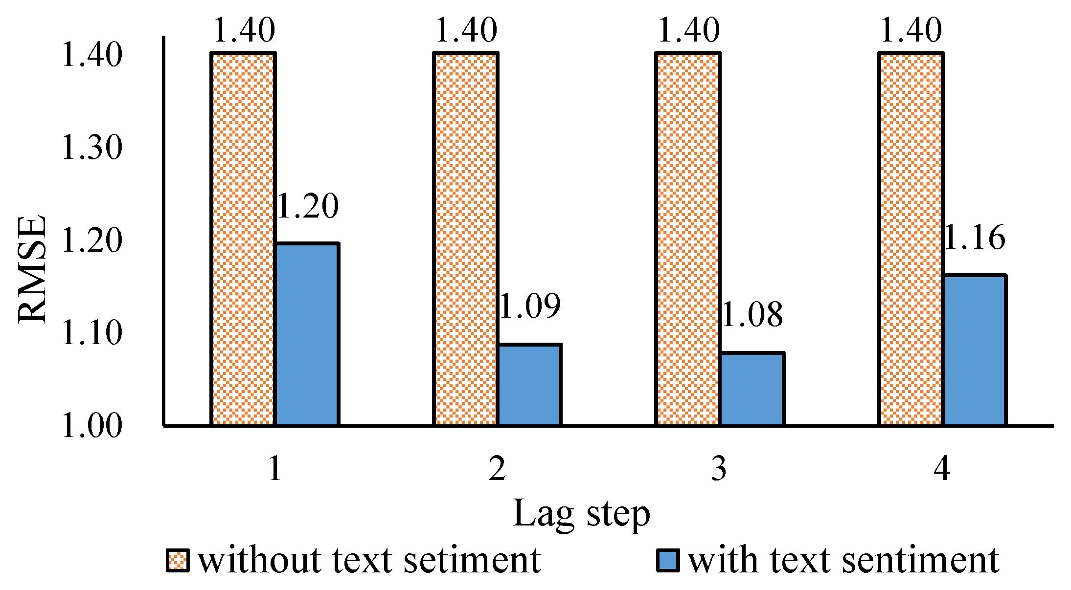
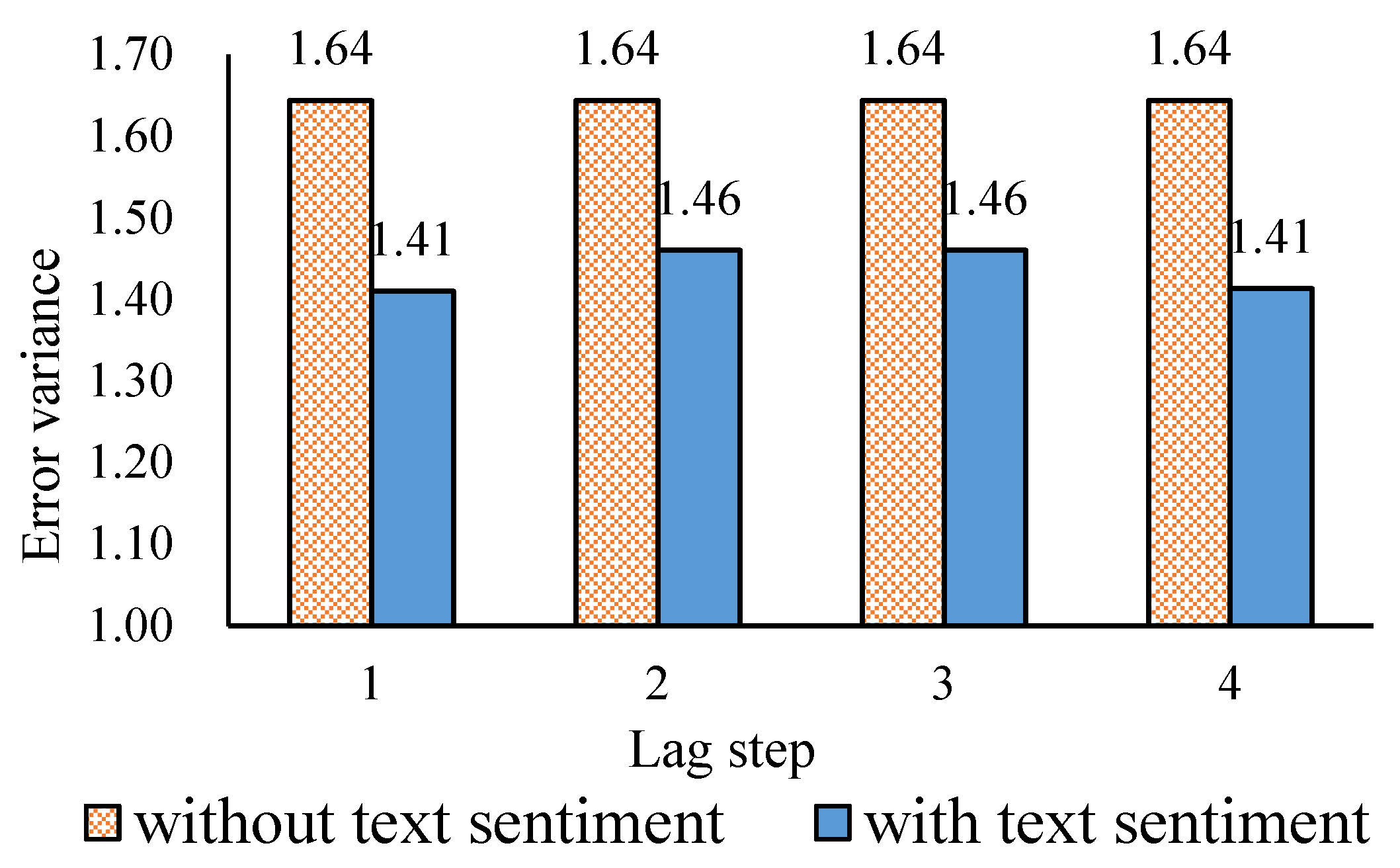
3.4. The Effect of Comprehensive Text Sentiment
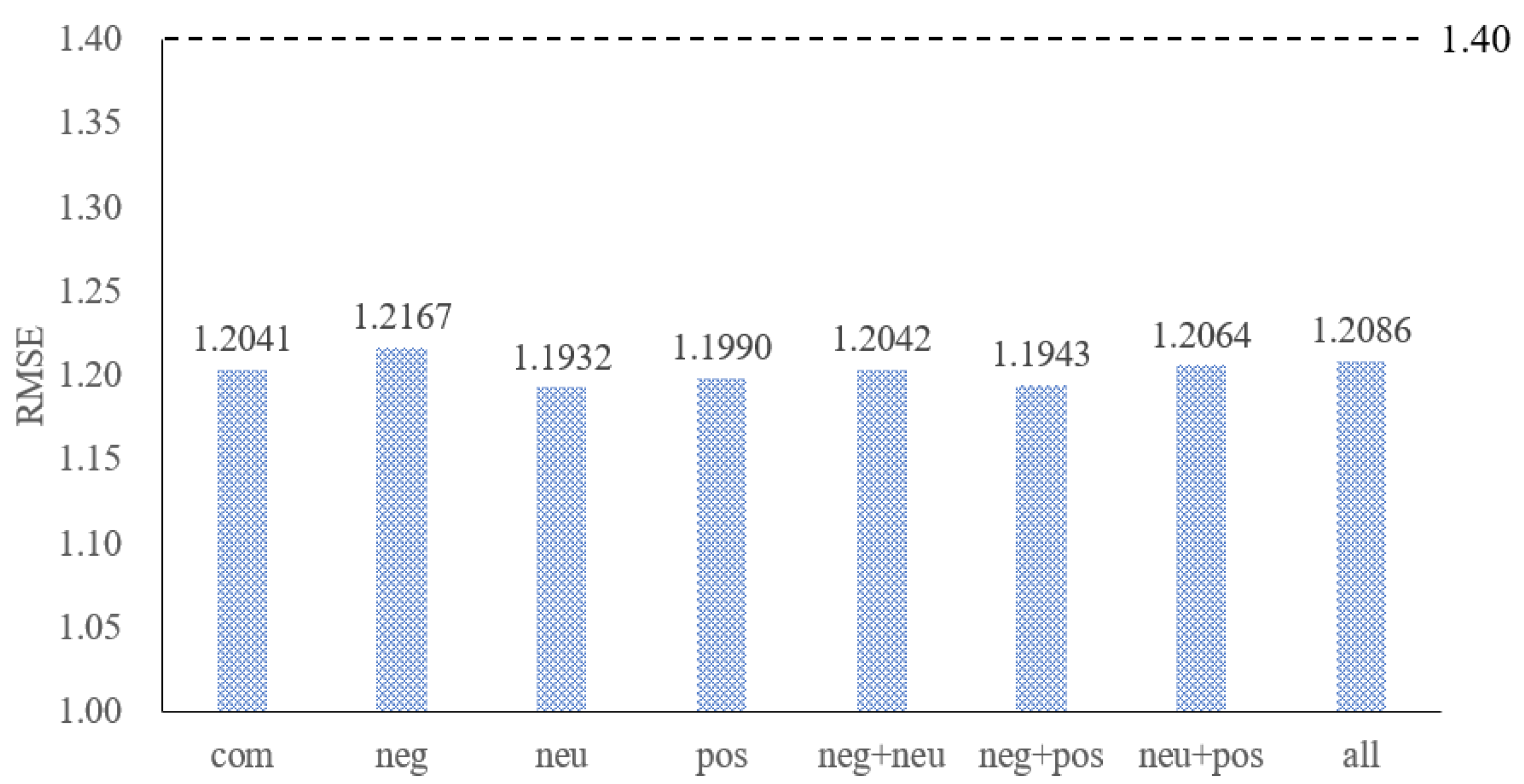
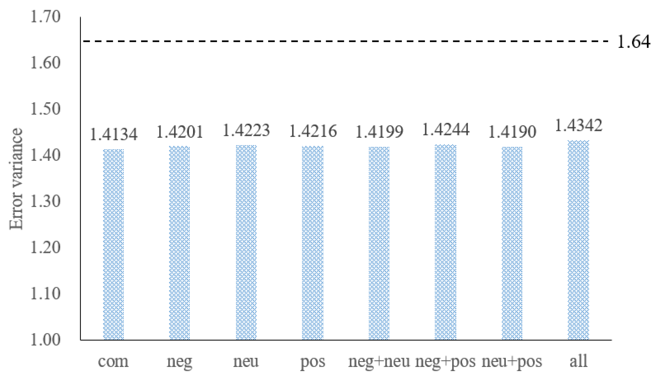
3.5. The Effect of Different Types of Text Sentiment
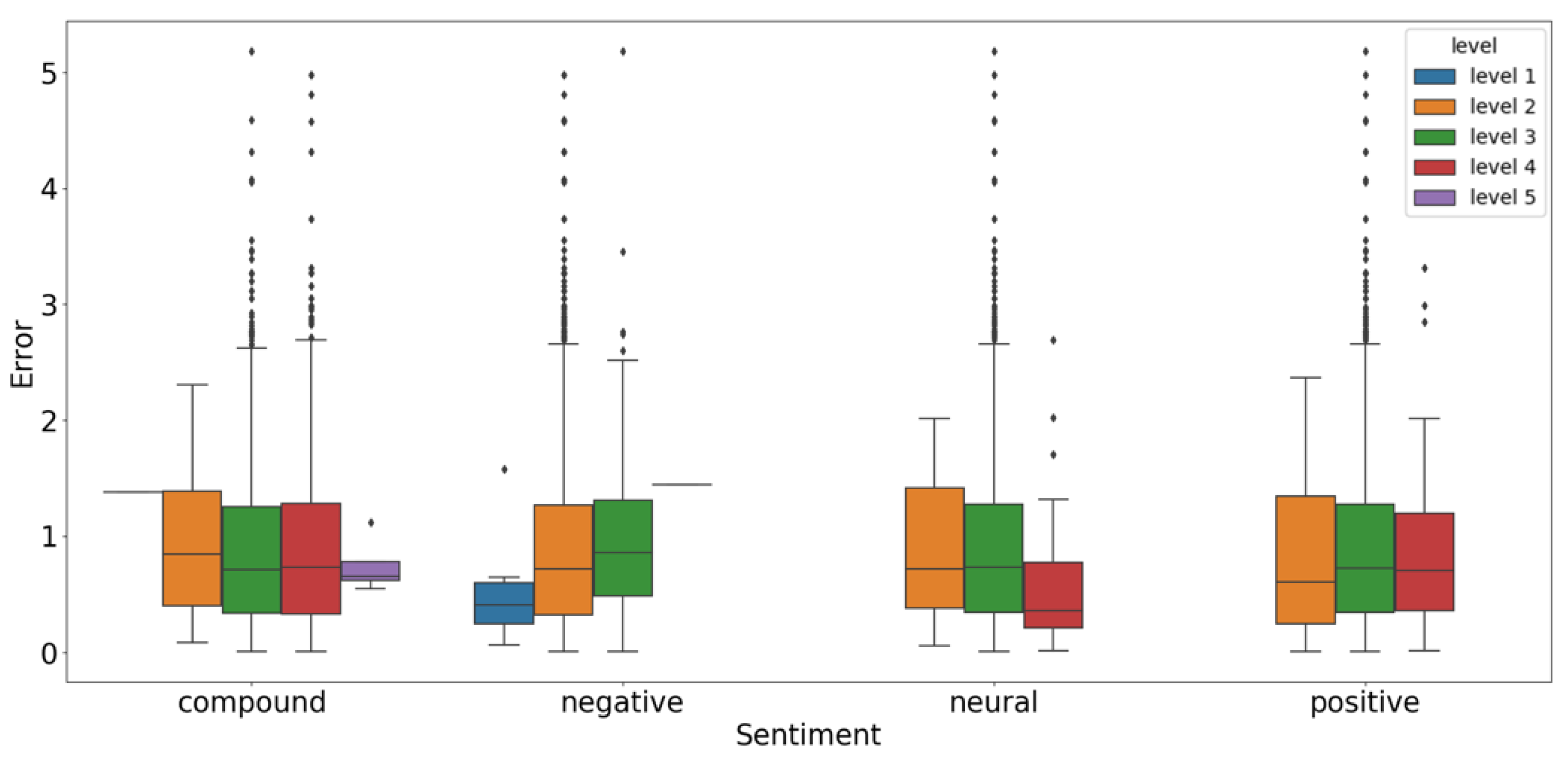
3.6. The Effect of Text Sentiment with Different Strength
4. Conclusions
Author Contributions
Funding
Acknowledgments
Conflicts of Interest
References
- Vo, D.H.; Vu, T.N.; McAleer, M. Modeling the Relationship between Crude Oil and Agricultural Commodity Prices. Energies 2019, 12, 1344. [Google Scholar] [CrossRef]
- Tule, M.K.; Ndako, U.B.; Onipede, S.F. Oil price shocks and volatility spillovers in the Nigerian sovereign bond market. Rev. Financ. Econ 2017, 35, 57–65. [Google Scholar] [CrossRef]
- Panas, E.; Ninni, V. Are oil markets chaotic? A non-linear dynamic analysis. Energy Econ. 2004, 22, 549–568. [Google Scholar] [CrossRef]
- Adrangi, B.; Chatrath, A.; Dhanda, K.K.; Raffiee, K. Chaos in oil prices? Evidence from futures markets. Energy Econ. 2001, 23, 405–425. [Google Scholar] [CrossRef]
- Zhao, L.T.; Liu, K.; Duan, X.L.; Li, M.F. Oil Price Risk Evaluation Using a Novel Hybrid Model Based on Time-varying Long Memory. Energy Econ. 2019, 81, 71–78. [Google Scholar] [CrossRef]
- Kayalar, D.E.; Küçüközmen, C.C.; Selcuk-Kestel, A.S. The impact of crude oil prices on financial market indicators: Copula approach. Energy Econ. 2017, 61, 162–173. [Google Scholar] [CrossRef]
- Hong, M.; Ramchander, S.; Wang, T.; Yang, D. Influential Factors in Crude Oil Price Forecasting. Energy Econ. 2017, 68, 77–88. [Google Scholar]
- Zhao, L.T.; Wang, Y.; Guo, S.Q.; Zeng, G.R. A novel method based on numerical fitting for oil price trend forecasting. Appl. Energy 2018, 220, 154–163. [Google Scholar] [CrossRef]
- Naser, H. Estimating and forecasting the real prices of crude oil: A data rich model using a dynamic model averaging (DMA) approach. Energy Econ. 2016, 56, 75–87. [Google Scholar] [CrossRef]
- Gabralla, L.A.; Jammazi, R.; Abraham, A. Oil price prediction using ensemble machine learning. In Proceedings of the International Conference on Computing, Electrical and Electronic Engineering (ICCEEE), Khartoum, Sudan, 26–28 August 2013; pp. 674–679. [Google Scholar]
- Wang, M.; Zhao, L.; Du, R.; Wang, C.; Chen, L.; Tian, L. A novel hybrid method of forecasting crude oil prices using complex network science and artificial intelligence algorithms. Appl. Energy 2018, 220, 480–495. [Google Scholar] [CrossRef]
- Yu, L.; Wei, D.; Ling, T. A novel decomposition ensemble model with extended extreme learning machine for crude oil price forecasting. Eng. Appl. Artif. Intell. 2016, 47, 110–121. [Google Scholar] [CrossRef]
- Huang, S.; An, H.; Huang, X.; Wang, Y. Do all sectors respond to oil price shocks simultaneously? Appl. Energy 2018, 227, 393–402. [Google Scholar] [CrossRef]
- Ji, Q.; Guo, J.F. Oil price volatility and oil-related events: An Internet concern study perspective. Appl. Energy 2015, 137, 256–264. [Google Scholar] [CrossRef]
- Lee, H.; Surdeanu, M.; MacCartney, B.; Jurafsky, D. On the Importance of Text Analysis for Stock Price Prediction. In Proceedings of the Ninth International Conference on Language Resources and Evaluation, Reykjavik, Iceland, 26–31 May 2014; pp. 1170–1175. [Google Scholar]
- Kumar, B.S.; Ravi, V. A survey of the applications of text mining in financial domain. Knowl. Based Syst. 2016, 114, 128–147. [Google Scholar] [CrossRef]
- Fung, G.P.C.; Yu, J.X.; Lam, W. News sensitive stock trend prediction. In Proceedings of the Pacific-Asia Conference on Knowledge Discovery and Data Mining, Taipei, Taiwan, 6–8 May 2002; pp. 481–493. [Google Scholar]
- Liu, L.; Wu, J.; Li, P.; Li, Q. A social-media-based approach to predicting stock comovement. Expert Syst. Appl. 2015, 42, 3893–3901. [Google Scholar] [CrossRef]
- Junqué de Fortuny, E.; De Smedt, T.; Martens, D.; Daelemans, W. Evaluating and understanding text-based stock price prediction models. Inf. Process. Manag. 2014, 50, 426–441. [Google Scholar] [CrossRef]
- Yao, T.; Zhang, Y.J.; Ma, C.Q. How does investor attention affect international crude oil prices? Appl. Energy 2017, 205, 336–344. [Google Scholar] [CrossRef]
- Wang, J.; Athanasopoulos, G.; Hyndman, R.J.; Wang, S. Crude oil price forecasting based on internet concern using an extreme learning machine. Int. J. Forecast. 2018, 34, 665–677. [Google Scholar] [CrossRef]
- Nassirtoussi, A.K.; Aghabozorgi, S.; Wah, T.Y.; Ngo, D.C.L. Text mining for market prediction: A systematic review. Expert Syst. Appl. 2014, 41, 7653–7670. [Google Scholar] [CrossRef]
- Chen, W.; Cai, Y.; Lai, K.; Xie, H. A Topic-Based Sentiment Analysis Model to Predict Stock Market Price Movement Using Weibo Mood. In Web Intelligence; IOS Press: Amsterdam, The Netherlands, 2016; pp. 287–300. [Google Scholar]
- Nguyen, T.H.; Shirai, K.; Velcin, J. Sentiment analysis on social media for stock movement prediction. Expert Syst. Appl. 2015, 42, 9603–9611. [Google Scholar] [CrossRef]
- Tetlock, P.C. Giving content to investor sentiment: The role of media in the stock market. J. Financ. 2007, 62, 1139–1168. [Google Scholar] [CrossRef]
- Ho, K.Y.; Shi, Y.; Zhang, Z. How does news sentiment impact asset volatility? Evidence from long memory and regime-switching approaches. N. Am. J. Econ. Financ. 2013, 26, 436–456. [Google Scholar] [CrossRef]
- Li, J.; Xu, Z.; Xu, H.; Tang, L.; Yu, L. Forecasting Oil Price Trends with Sentiment of Online News Articles. Asia Pac. J. Oper. Res. 2016, 91, 1081–1087. [Google Scholar] [CrossRef]
- Yu, L.; Wang, S.; Lai, K.K. A Rough-Set-Refined Text Mining Approach for Crude Oil Market Tendency Forecasting. Int. J. Knowl. Syst. Sci. 2005, 2, 33–46. [Google Scholar]
- Wex, F.; Widder, N.; Liebmann, M.; Neumann, D. Early warning of impending oil crises using the predictive power of online news stories. In Proceedings of the 46th Hawaii International Conference on System Sciences, Wailea, Maui, HI, USA, 7–10 January 2013; pp. 1512–1521. [Google Scholar]
- Li, X.; Shang, W.; Wang, S. Text-based crude oil price forecasting: A deep learning approach. Int. J. Forecast. 2018, 35, 1548–1560. [Google Scholar] [CrossRef]
- Hutto, C.J.; Gilbert, E. VADER: A Parsimonious Rule-Based Model for Sentiment Analysis of Social Media Text. In Proceedings of the Eighth International Conference on Weblogs and Social Media, Ann Arbor, MI, USA, 1–4 June 2014. [Google Scholar]
- Song, K.; Feng, S.; Gao, W.; Wang, D.; Chen, L.; Zhang, C. Build Emotion Lexicon from Microblogs by Combining Effects of Seed Words and Emoticons in a Heterogeneous Graph. In Proceedings of the 26th ACM Conference on Hypertext & Social Media, Guzelyurt, Turkey, 1–4 September 2015; pp. 283–292. [Google Scholar]
- Song, K.; Shi, F.; Wei, G.; Wang, D.; Ge, Y.; Wong, K.F. Personalized Sentiment Classification Based on Latent Individuality of Microblog Users. In Proceedings of the Twenty-Fourth International Joint Conference on Artificial Intelligence, Buenos Aires, Argentina, 25–31 July 2015; pp. 2277–2283. [Google Scholar]
- Soleymani, M.; Garcia, D.; Jou, B.; Schuller, B.; Chang, S.F. A Survey of Multimodal Sentiment Analysis. Image Vision Comput. 2017, 65, 3–14. [Google Scholar] [CrossRef]
- Ling, T.; Yao, W.; Yu, L. A non-iterative decomposition-ensemble learning paradigm using RVFL network for crude oil price forecasting. Appl. Soft Comput. 2017, 70, 1097–1108. [Google Scholar]
- Haworth, J.; Shawe-Taylor, J.; Cheng, T.; Wang, J. Local online kernel ridge regression for forecasting of urban travel times. Transp. Res. Part C 2014, 46, 151–178. [Google Scholar] [CrossRef]
- Jie, W.; Ren, G.; Liu, J.; Hu, Q.; Yu, D. Ultra-short-term wind speed prediction based on multi-scale predictability analysis. Clust. Comput. 2016, 19, 741–755. [Google Scholar]
- Feng, M.; Jing, L.; Wahab, M.I.M.; Zhang, Y. Forecasting the aggregate oil price volatility in a data-rich environment. Econ. Model. 2018, 72, 320–332. [Google Scholar]
- Ludwig, N.; Feuerriegel, S.; Neumann, D. Putting Big Data analytics to work: Feature selection for forecasting electricity prices using the LASSO and random forests. J. Decis. Syst. 2015, 24, 19–36. [Google Scholar] [CrossRef]
- Yu, L.; Xu, H.; Ling, T. LSSVR ensemble learning with uncertain parameters for crude oil price forecasting. Bibliometrics 2017, 56, 692–701. [Google Scholar] [CrossRef]
- Xie, W.; Yu, L.; Xu, S.; Wang, S. A New Method for Crude Oil Price Forecasting Based on Support Vector Machines. In International Conference on Computational Science; Springer: Berlin/Heidelberg, Germany, 2006; pp. 444–451. [Google Scholar]
- Shi, S.; Liu, W.; Jin, M. Stock price forecasting using a hybrid ARMA and BP neural network and Markov model. In Proceedings of the 14th International Conference on Communication Technology, Chengdu, China, 9–11 November 2012; pp. 981–985. [Google Scholar]
- Yi, B.; Liu, W. Research on Prediction Methods of Residential Real Estate Price Based on Improved BPNN. In Proceedings of the International Conference on Smart Grid and Electrical Automation (ICSGEA), Zhangjiajie, China, 11–12 August 2016. [Google Scholar]
- Booth, A.; Gerding, E.; Mcgroarty, F. Automated trading with performance weighted random forests and seasonality. Expert Syst. Appl. 2014, 41, 3651–3661. [Google Scholar] [CrossRef]
- Wang, J.; Wang, J. Forecasting energy market indices with recurrent neural networks: Case study of crude oil price fluctuations. Energy 2016, 102, 365–374. [Google Scholar] [CrossRef]
- Zhao, L.T.; Zeng, G.R.; He, L.Y.; Meng, Y. Forecasting Short-Term Oil Price with a Generalised Pattern Matching Model Based on Empirical Genetic Algorithm. Comput. Econ. 2018. [Google Scholar] [CrossRef]


| Variable Name | Remark |
|---|---|
| The comprehensive text sentiment score calculated by text sentiment analysis | |
| The negativeext sentiment score calculated by text sentiment analysis | |
| The neutral text sentiment score obtained by text sentiment analysis | |
| The positive texsentiment score calculated by text sentiment analysis |
| Variable Name | Remark |
|---|---|
| The web text comprehensive sentiment at the given time t | |
| The web text negative sentiment at the given time t | |
| The web text neutral sentiment at the given time t | |
| The web text positive sentiment at the given time t |
| Model | Advantages | Disadvantages | Reference |
|---|---|---|---|
| Ridge | Highly interpretable, High stability, Fast calculation, Solve multi-collinearity problems. | Linear model, Biased estimation, Unable to parse complex relationships, Predicted performance is limited, Easy to produce overfitting. | Ling et al. [35]; Haworth et al. [36]; Jie et al. [37]. |
| LASSO | Highly interpretable, Irrelevant feature screening, The case of overfitting is handled. | Linear model, Unable to parse complex relationships, Biased estimation, Predicted performance is limited, Loss function is not continuously steerable. | Hong et al. [7]; Feng et al. [38]; Ludwig et al. [39]. |
| SVR | Non-linear, The kernel function is flexible, Control the appearance of extreme errors. | Sensitive to parameters, Large number of hyperparameters. | Wang et al. [11]; Yu et al. [40]; Xie et al. [41]. |
| BPNN | Non-linear, The model structure is flexible, Strong ability to mine relationships, Fewer constraints, High prediction accuracy. | Data volume requirements, Easy to over-fit, Low interpretability. | Wang et al. [11]; Shi et al. [42]; Yi and Liu [43] |
| RF | Highly non-linear, High stability, Highly interpretable, High precision. | The number of hyperparameters is large, Data volume requirements, Easy to over-fit, Long training time. | Ludwig et al. [39]; Booth et al. [44] |
| Statistics | Amount | Mean | Maximum | Minimum | Standard Deviation |
|---|---|---|---|---|---|
| Value | 1447 | 71.38 | 118.90 | 26.01 | 26.39 |
| Title | Content |
|---|---|
| Websites | Reuters, UPI |
| Search terms | oil price, oil market, petroleum, gas, gasoline, benzine, diesel, fuel, Paraffin, kerosene, coal oil, OPEC WTI Brent, fossil, Mobil, Royal Dutch, Shell Group of Companies, Total, Chevron, Gazprom, Phillips |
| Amount | 107,298 documents (a total of 38,075,959 words) |
| Date | 1 January 2013–31 August 2018 |
| Algorithm. | RMSE | MAPE | EV |
|---|---|---|---|
| BPNN | 1.1872 | 1.2691 | 1.4090 |
| NAIVE | 1.1936 | 1.2796 | 1.4213 |
| LASSO | 1.1944 | 1.2841 | 1.4179 |
| Ridge | 1.1960 | 1.2812 | 1.4264 |
| ARIMA | 1.1971 | 1.2836 | 1.4298 |
| SVR | 1.4223 | 1.5364 | 1.7599 |
| RF | 1.8774 | 2.0564 | 3.2743 |
| Sentiment | Level | Support | Mean Error | Variance of Error | Error > 2 | Error > 3 | Error > 4 | Error > 5 |
|---|---|---|---|---|---|---|---|---|
| Compound | 1 | 1 | 1.3793 | 0.0000 | 0.00% | 0.00% | 0.00% | 0.00% |
| 2 | 24 | 0.8933 | 0.3653 | 4.17% | 0.00% | 0.00% | 0.00% | |
| 3 | 766 | 0.9145 | 0.6045 | 9.79% | 1.96% | 0.65% | 0.13% | |
| 4 | 652 | 0.8847 | 0.5573 | 7.98% | 1.53% | 0.61% | 0.00% | |
| 5 | 4 | 0.7440 | 0.0492 | 0.00% | 0.00% | 0.00% | 0.00% | |
| Negative | 1 | 6 | 0.5512 | 0.2442 | 0.00% | 0.00% | 0.00% | 0.00% |
| 2 | 1347 | 0.8935 | 0.5701 | 8.76% | 1.71% | 0.59% | 0.00% | |
| 3 | 93 | 1.0193 | 0.6909 | 10.75% | 2.15% | 1.08% | 1.08% | |
| 4 | 1 | 1.4458 | 0.0000 | 0.00% | 0.00% | 0.00% | 0.00% | |
| 5 | 0 | - | - | - | - | - | - | |
| Neutral | 1 | 0 | - | - | - | - | - | - |
| 2 | 17 | 0.8880 | 0.3646 | 5.88% | 0.00% | 0.00% | 0.00% | |
| 3 | 1402 | 0.9064 | 0.5820 | 8.92% | 1.78% | 0.64% | 0.07% | |
| 4 | 28 | 0.6177 | 0.4144 | 7.14% | 0.00% | 0.00% | 0.00% | |
| 5 | 0 | - | - | - | - | - | - | |
| Positive | 1 | 0 | - | - | - | - | - | - |
| 2 | 40 | 0.7981 | 0.4419 | 7.50% | 0.00% | 0.00% | 0.00% | |
| 3 | 1336 | 0.9065 | 0.5878 | 9.06% | 1.80% | 0.67% | 0.07% | |
| 4 | 71 | 0.8470 | 0.4568 | 5.63% | 1.41% | 0.00% | 0.00% | |
| 5 | 0 | - | - | - | - | - | - |
© 2019 by the authors. Licensee MDPI, Basel, Switzerland. This article is an open access article distributed under the terms and conditions of the Creative Commons Attribution (CC BY) license (http://creativecommons.org/licenses/by/4.0/).
Share and Cite
Zhao, L.-T.; Zeng, G.-R.; Wang, W.-J.; Zhang, Z.-G. Forecasting Oil Price Using Web-based Sentiment Analysis. Energies 2019, 12, 4291. https://doi.org/10.3390/en12224291
Zhao L-T, Zeng G-R, Wang W-J, Zhang Z-G. Forecasting Oil Price Using Web-based Sentiment Analysis. Energies. 2019; 12(22):4291. https://doi.org/10.3390/en12224291
Chicago/Turabian StyleZhao, Lu-Tao, Guan-Rong Zeng, Wen-Jing Wang, and Zhi-Gang Zhang. 2019. "Forecasting Oil Price Using Web-based Sentiment Analysis" Energies 12, no. 22: 4291. https://doi.org/10.3390/en12224291
APA StyleZhao, L.-T., Zeng, G.-R., Wang, W.-J., & Zhang, Z.-G. (2019). Forecasting Oil Price Using Web-based Sentiment Analysis. Energies, 12(22), 4291. https://doi.org/10.3390/en12224291