An Enhanced Method to Assess MPC Performance Based on Multi-Step Slow Feature Analysis

Abstract

Due to the wide application of model predictive control (MPC) in industrial processes, the assessment of MPC performance is essential to ensure product quality and improve energy efficiency. Recently, the slow feature analysis (SFA) algorithm has been successfully applied to assess the performance of MPC. However, the disadvantage of the traditional SFA-based predictable index is that it can only extract one-step predictable information in the monitored variables. In order to better mine the predictable information contained in the monitored variables with large lag, an enhanced method to assess MPC performance based on multi-step SFA (MSSFA) is proposed. Based on the relationship between the slowness of slow features (SFs) and data predictability, an MSSFA model SFA(τ) is built through extending the temporal derivatives of the SFs from one step to multiple steps to extract multi-step predictable information in the monitored variables, which is used to construct a multi-step predictable index. Then, the predictable information in the SFs is further extracted for enhancing the multi-step predictable index to improve its sensitivity to performance changes. The effectiveness of the proposed method has been verified through two process simulation examples.

1. Introduction

Model Predictive Control (MPC) is a mature technology that has been widely implemented for advanced control of many processes, such as oil refining, chemical, advanced manufacturing, energy, environment, aerospace, medicine [1,2]. At each control interval an MPC algorithm computes the future control actions by minimizing an objective function over a finite prediction horizon according to the historical information and future response of the process model [3]. This type of control algorithm has the ability to handle multiple interacting variables, constraints, large delay and complex dynamic processes [4].

MPC with good performance can achieve more efficient raw material and energy usage per unit of product [5]. Studies have shown that it is very common to quote energy savings of 1–4% through implementation of advanced control and other process control technologies [6]. However, in the investigated plants over the 600,000 loops, up to 75% of the control loops are not providing benefits due to the poor control performance [7]. In industrial applications, MPC performance will gradually decrease over time due to various factors such as sensor failure and equipment wear, etc. [8], which can lead to a decline in product quality and an increase in energy consumption [5]. Thus, it is important to assess the MPC performance and maintain its performance in an optimal state.

In recent years, performance assessment techniques have received extensive attention and rapid development in different industrial fields, such as the processing industry [9], energy and power fields [10,11]. Among them, the control performance assessment (CPA) technique for MPC in the process industry is an important branch and the number of CPM tools installed in the industrial process is increasing [12]. Over the past three decades, various CPA methods or benchmarks for MPC have been proposed and developed. Among these methods, model-based CPA benchmarks were first proposed for evaluating MPC performance, such as generalized-minimum variance control benchmark [13] and linear-quadratic Gaussian benchmark [14]. Both benchmarks give a theoretical performance bound with respect to the system output variance and the controller output variance, which helps to focus on product quality and actuator wear. In addition, Julien et al. proposed two performance curves, an old-controller-new-model performance curve and a new-controller-new-model performance curve to assess the potential improvement performance of MPC [15]. However, model-based benchmarks typically require a complete plant model to calculate performance index. Although the process model can be estimated from closed-loop data in some cases, this method usually requires a lot of cost and time [16] and requires the additional information such as the knowledge of the time delay or an external excitation signal to create a sufficient signal-to-noise ratio [5]. Therefore, user-specified CPA benchmarks were proposed to get rid of the dependence on the plant model. By comparing the actual MPC performance with the expected performance or design performance specified by the field engineer, the expectation-case performance index and design-case performance index were presented separately [17,18]. Similar to the knowledge-based system, user-specified benchmarks also require extensive knowledge and experience from the field engineer, which limits their range of applications.

Due to the development of sensor measurement and control technology, data-driven multivariate statistical methods, such as principle component analysis (PCA) [19,20] and partial least squares (PLS) [21,22], have been introduced into the CPA field and have been used to assess the MPC performance. The data-driven CPA methods assess the performance by deepening the performance information contained in the monitored variables. They have the advantages of simple implementation and wide application range, and have received more and more attention from researchers and engineers [23]. Zhang and Li [24] combine a PCA model and an autoregressive moving average filter to monitor MPC performance. Zhao et al. [25] developed multiple PLS models for performance monitoring of processes with multiple operating modes. Through utilizing historical output data, a statistical covariance-based index was proposed by Yu and Qin [26,27]. Then, Tian et al. improved this index and proposed an improved covariance index based on 2-norm [3]. In order to discover abnormal changes in the distribution features of covariance matrices, a dissimilarity analysis based method [28] and a hypothesis test based method [29] were proposed by Li et al. and Yan et al., respectively. Wu [30] established performance monitoring index based on Kullback–Leibler divergence. Xu et al. [31,32] use distance similarity factor-based on mahalanobis distance to assess MPC performance.

However, above traditional CPA methods only considered the steady state information of the process data without deeper mining of the temporal dynamic information therein. In order to solve this problem, Shang et al. [33,34] proposed a method based on slow feature analysis (SFA) to monitor control performance in both of the steady state and temporal dynamic dimensions. This method was successfully applied to batch processes monitoring [35], as well as soft sensor modeling [36]. Zhao et al. [37] proposed a fine-scale assessment method of glycemic control performance by analyzing the temporal changing speed of the monitored data. By analyzing the process dynamics directly related to closed-loop control from quality-relevant view for industrial processes, Qin and Zhao [38] proposed a fine-scale monitoring method of process performance status. Although the SFA-based CPA method has the ability to monitor changes in control performance, it does not point the direction of performance changes, that is, whether the control performance is getting better or worse [34]. For the purpose of overcoming this shortcoming, an SFA-based predictable index was presented by Shang et al. [39]. The SFA-based predictable index assesses MPC performance on the basis of the relationship between the slowness of slow features (SFs) and the predictability of monitored variables. In industrial applications, MPC is usually applied to large time-delay systems, so that relevant temporal predictable information also exists between SFs with different step intervals. For example, if a process has two sample time delays, then the compensation control action will not take effect on the output until two steps later, which prevents the complete compensation of the predictable content of the output in time. However, due to the limitation of the traditional SFA model structure, the predictable index only extracts predictable information between adjacent points of SFs, that is, it essentially only extracts one-step predictability in monitored variables but ignores the multi-step predictable information.

In order to extract the multi-step predictable information in monitored variables to overcome the shortcomings of the traditional SFA-based performance assessment method, a multi-step SFA (MSSFA) is proposed to assess MPC performance, which can be used to construct the multi-step predictable index. Firstly, by extending the temporal derivatives of the SFs from one step to multiple steps, an MSSFA model SFA(τ) is built and the corresponding multi-step predictable index In(τ) is constructed. Then, the SFs of SFA(τ) can be formulated as a prediction model similar to autoregressive (AR). This prediction model is used to predict SFs and the prediction error can be obtained. Thirdly, a new MSSFA model SFA_e(τ_e) with the prediction error as input is developed and the corresponding multi-step predictable index In_e(τ) is built to extract the predictable information in prediction error. Finally, by incorporating In(τ) and In_e(τ), an enhanced multi-step predictable index In_pre(τ) is finally established. Considering the time-delay system that is common in industrial processes, the proposed method can effectively extract multi-step predictable information in data for assessment of MPC performance.

The rest of this article is organized as follows. Firstly, the traditional SFA-based predictable index is briefly reviewed. Subsequently, the multi-step predictable index for MPC performance assessment is introduced. Afterward, simulation studies and discussions are given. Finally, the conclusions are presented.

2. Traditional SFA-Based Predictable Index for MPC Performance Assessment

2.1. The Basic Principle of Traditional SFA

Formally, the mathematical principle of the SFA algorithm can be stated as follows: given an m-dimensional stochastic and ergodic time series $\mathit{x}(t)={[x_1(t),\cdots ,x_m(t)]}^{\mathrm{T}}$, the slow feature $s_j(t)$ is extracted from $\mathit{x}(t)$ by using a feature function $g_j(\mathit{x})(j=1,\cdots ,m)$ as below:

$$s_j(t)=g_j(\mathit{x}(t)),$$

(1)

where the output signal $s_j(t)$ varies as slowly as possible by minimizing the average squared temporal variation:

$${\displaystyle \underset{g_j(•)}{\min }}\Delta (s_j)={\displaystyle \underset{g_j(•)}{\min }}{\langle {\dot{s}}_j^2\rangle }_t$$

(2)

under the constraints:

$${\langle s_j(t)\rangle }_t=0,$$

(3)

$${\langle s_j^2(t)\rangle }_t=1,$$

(4)

$$\forall i\ne j,{\langle s_i(t)s_j(t)\rangle }_t=0,$$

(5)

where $\Delta (\cdot )$ is defined as slowness of a time series. The symbol ${\langle \cdot \rangle }_t$ stands for an expectation with respect to time. ${\dot{s}}_j(t)$ denotes the temporal derivative of $s_j(t)$. For discrete time series, ${\dot{s}}_j(t)$ can be calculated as:

$${\dot{s}}_j(t)=s_j(t)-s_j(t-1).$$

(6)

The role of constraints Equation (3) and Equation (4) is to ensure zero mean and unit variance for each SF and to avoid the trivial solution. The goal of constraint in Equation (5) is to make SFs independent of each other. Descending order of ${\left\{s_j\right\}}_{j=1}^m$ is adopted, so that $s_1$ is the slowest SF, and $s_2$ is the second slowest SF, etc.

For linear SFA algorithm, SFs can be computed as:

$$s_j(t)={\mathit{w}}_j^{\mathrm{T}}\mathit{x}(t)={\displaystyle \sum _{i=1}^m{w}_{ji}}{x}_i(t),$$

(7)

where ${\mathit{w}}_j(j=1,\cdots ,m)$ is the feature vector of $s_j(t)$. The original input data is normalized in the data preprocessing stage, substitute Equation (7) into Equation (1) and Equation (4) to yield:

$$\Delta (s_j)={\langle {\dot{s}}_j^{}{(t)}^2\rangle }_t={\mathit{w}}_j^{\mathrm{T}}{\langle \dot{\mathit{x}}(t)\dot{\mathit{x}}{(t)}^{\mathrm{T}}\rangle }_t{\mathit{w}}_j^{}={\mathit{w}}_j^{\mathrm{T}}\mathit{A}{\mathit{w}}_j^{},$$

(8)

$${\langle s_j^2(t)\rangle }_t={\mathit{w}}_j^{\mathrm{T}}{\langle \mathit{x}(t)\mathit{x}{(t)}^{\mathrm{T}}\rangle }_t{\mathit{w}}_j^{}={\mathit{w}}_j^{\mathrm{T}}\mathit{B}{\mathit{w}}_j^{}=1,$$

(9)

where $\mathit{A}={\langle \dot{\mathit{x}}(t)\dot{\mathit{x}}{(t)}^{\mathrm{T}}\rangle }_t$, $\mathit{B}={\langle \mathit{x}(t)\mathit{x}{(t)}^{\mathrm{T}}\rangle }_t$. According to Equation (8) and Equation (9), the optimal objective function in Equation (2) of SFA can be rewritten as:

$${\displaystyle \underset{w_j}{\min }}\Delta (s_j)={\displaystyle \underset{w_j}{\min }}\frac{{\langle {\dot{s}}_j^{}{(t)}^2\rangle }_t}{{\langle s_j^2\rangle }_t}={\displaystyle \underset{w_j}{\min }}\frac{{\mathit{w}}_j^{\mathrm{T}}\mathit{A}{\mathit{w}}_j^{}}{{\mathit{w}}_j^{\mathrm{T}}\mathit{B}{\mathit{w}}_j^{}}.$$

(10)

From Equation (10), it can be seen that solving the objective function in Equation (2) is equivalent to solving the following generalized eigenvalue problem [33]:

$$\mathit{A}\mathit{W}=\mathit{B}\mathit{W}\mathbf{\Omega },$$

(11)

where $\mathit{W}={[{\mathit{w}}_1,\cdots ,{\mathit{w}}_m]}^{\mathrm{T}}$, $\mathbf{\Omega }=\mathrm{diag}\{{\omega }_1,\cdots ,{\omega }_m\}$, ${\omega }_j$ is the generalized eigenvalue and ${\omega }_1<{\omega }_2<\cdots <{\omega }_m$. The generalized eigenvalue can be used as a measure of slowness:

$$\Delta (s_j)=\frac{{\mathit{w}}_j^{\mathrm{T}}\mathit{A}{\mathit{w}}_j^{}}{{\mathit{w}}_j^{\mathrm{T}}\mathit{B}{\mathit{w}}_j^{}}=\frac{{\mathit{w}}_j^{\mathrm{T}}{\mathit{\omega }}_j\mathit{B}{\mathit{w}}_j^{}}{{\mathit{w}}_j^{\mathrm{T}}\mathit{B}{\mathit{w}}_j^{}}={\omega }_j.$$

(12)

The smallest eigenvalue corresponds to the slowest SF.

2.2. Predictable Index Based on Traditional SFA

As pointed out in [40], if a closed-loop output is highly predictable, then one should design a better controller to compensate for the predictable content. Should a better controller be implemented, then the closed-loop output would have been less predictable [40]. Therefore, the high predictability of a closed-loop output implies the potential to improve its performance. In addition, for MPC controllers, the accuracy of the model is one of the main factors affecting MPC performance. If the model is completely accurate, the future output of the process can be predicted completely accurately. At this situation, the model prediction error is only driven by random measurement noise, and its predictability is very low. On the contrary, its predictability will be higher. Therefore, the model prediction error can also reflect the performance of the MPC controller [39]. Thus, if the closed-loop output and model prediction error are highly predictable, the performance of this MPC controller is poor, and vice versa.

The higher the predictability, the worse the control performance [39,40]. Based on this idea, the traditional predictable index based on SFA was proposed. The graphical structure of traditional SFA is shown in Figure 1:

For discrete input data, the slowness in objective function Equation (2) can be further derived as [39]:

$$\begin{array}{cc}\hfill \Delta \left(s_j\right)& ={\langle {\dot{s}}_j^2\rangle }_t\hfill \\ & ={\langle {(s_j(t+1)-s_j(t))}^2\rangle }_t\hfill \\ & =\left\{2{\langle s_j{(t)}^2\rangle }_t-2{\langle s_j(t+1)s_j(t)\rangle }_t\right\}\hfill \\ & =2-2{\rho }_j^{\mathrm{s}}(1)\hfill \end{array},$$

(13)

where ${\rho }_j^{\mathrm{s}}(1)$ is lag-1 autocorrelation of $s_j$. By substituting Equation (12) into Equation (13):

$${\omega }_j=2-2{\rho }_j^{\mathrm{s}}(1),$$

(14)

where ${\rho }_j^{\mathrm{s}}(1)\in [-1,1]$ and ${\omega }_j\in [0,4]$.

According to Equation (13), the objective function Equation (2) can be reformulated as follows:

$${\displaystyle \underset{w_j}{\max }}\overline{\Delta }(s_j)={\displaystyle \underset{w_j}{\max }}\left\{1-\frac{1}{2}\Delta \left(s_j\right)\right\}={\displaystyle \underset{w_j}{\max }}\left\{1-\frac{1}{2}{\omega }_j\right\}={\displaystyle \underset{w_j}{\max }}{\rho }_j^{\mathrm{s}}(1).$$

(15)

According to Equation (15), the slowest SF has the largest lag-1 autocorrelation. The time series with large autocorrelation is highly predictable. Thus, the slowest SF series has the greatest predictability. If ${\rho }_j^{\mathrm{s}}(1)$ is close to 0, and ${\omega }_j$ is close to 2, the corresponding SF $s_j$ is close to the white noise sequence and its predictability is close to zero.

Based on Equation (7), the correlation functions of SFs can be computed as follows:

$$\begin{array}{cc}\hfill {\rho }_{pq}^s(\tau )& ={\langle {\mathit{w}}_p^{\mathrm{T}}\mathit{x}(t+\tau ){\mathit{w}}_q^{\mathrm{T}}\mathit{x}(t)\rangle }_t\hfill \\ & ={\langle ({\displaystyle \sum _{j=1}^m{w}_{pj}}{x}_j(t+\tau ))({\displaystyle \sum _{i=1}^m{w}_{qi}}{x}_i(t))\rangle }_t\hfill \\ & ={\displaystyle \sum _{p=1}^m{\displaystyle \sum _{q=1}^m{w}_{pj}{w}_{qi}}}{\langle x_j(t+\tau )x_i(t)\rangle }_t\hfill \\ & ={\displaystyle \sum _{i=1}^m{w}_{pi}{w}_{qi}{\rho }_i^x(\tau )} 1\le p\le m, 1\le q\le m\hfill \end{array},$$

(16)

where ${\rho }_{pq}^s(\tau )$ is the lag-τ correlation between $s_p$ and $s_q$, ${\rho }_i^x(\tau )$ is the lag-τ autocorrelation of $x_i$. Let $p=q=j$, $\tau =1$, and substitute Equation (16) into Equation (15) to obtain the following formula:

$$\begin{array}{cc}\hfill {\displaystyle \underset{w_j}{\max }}\overline{\Delta }(s_j)& ={\displaystyle \underset{w_j}{\max }}{\rho }_j^s(1)\hfill \\ & ={\displaystyle \underset{w_j}{\max }}{\displaystyle \sum _{i=1}^m{w}_{ji}^2{\rho }_i^x(1)}\hfill \\ & ={\displaystyle \underset{w_j}{\max }}\left\{w_{j1}^2{\rho }_1^x(1)+w_{j2}^2{\rho }_2^x(1)+\dots +w_{jm}^2{\rho }_m^x(1)\right\}\hfill \end{array}$$

(17)

From Equation (17), it can be seen that if ${\rho }_1^x(1), {\rho }_2^x(1), \dots , {\rho }_m^x(1)$ are close to 0, i.e., the overall predictable information in monitored variables is low. ${\rho }_j^s(1)$ is close to 0, i.e., the predictability of $s_j$ is also low, and vice versa. Thereby, the predictability of $s_j$ can be used to express the predictability of monitored variables. Based on the distance relationship between the slowness of the slowest SF and the value 2, the traditional SFA-based predictable index is defined as [39]:

$$In(1)=1-{\left(\frac{{\omega }_{\min }-2}{2}\right)}^2,$$

(18)

where ${\omega }_{\min }$ is the slowness of the slowest SF and $0\le In(1)\le 1$. When $In(1)$ is close to 1, the predictability of monitored variables is low, and current control performance is good. When $In(1)$ is close to 0, the predictability of monitored variables is high, and current control performance is poor.

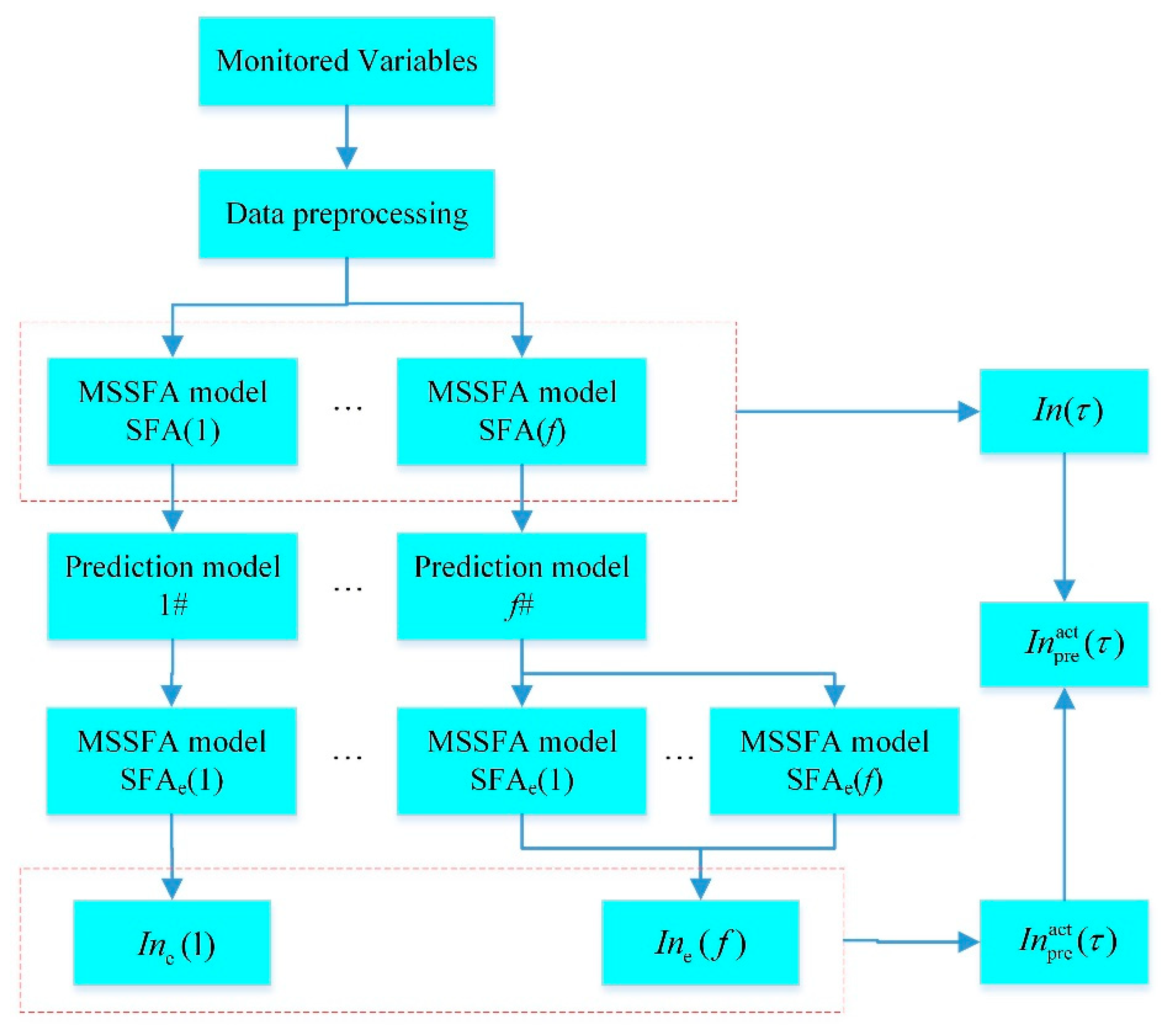
3. The Proposed Enhanced Multi-Step Predictable Index Based on Multi-Step SFA Method

However, according to Equation (6) and Equation (17), the traditional SFA method only focuses on the autocorrelation between adjacent points of SFs, that is, the traditional SFA-based predictable index only reveals one-step predictable information of monitored variables. In practice, for large time-delay systems, there is also predictable information between SFs with different step intervals. In order to mine the multi-step predictable information, a multi-step predictable index is proposed.

Firstly, the interval between the slow feature in Equation (6) is extended from one-step to multiple steps, and Equation (6) is redefined as:

$${\dot{s}}_j^{\tau }(t)=s_j(t)-s_j(t-\tau ), 0<\tau <f$$

(19)

where τ is the interval step, $f$ is the truncation step. Then multi-step SFA model SFA(τ) is built as

$$\begin{array}{cc}\hfill {\displaystyle \underset{w_j}{\min }}\Delta (s_j^{\tau })& ={\displaystyle \underset{w_j}{\min }}{\langle {\left\{{\dot{s}}_j^{\tau }\right\}}^2\rangle }_t\hfill \\ & ={\displaystyle \underset{w_j}{\min }}\left\{2-2{\rho }_j^{\mathrm{s}}(\tau )\right\}\hfill \\ & ={\displaystyle \underset{w_j}{\min }}{\omega }_j^{}(\tau )\hfill \end{array}$$

(20)

where ${\rho }_j^{\mathrm{s}}(\tau )$ is lag-τ autocorrelation of $s_j^{\tau }$, ${\omega }_j^{}(\tau )$ is the slowness of SFA(τ). The equivalent objective function is as follows:

$$\begin{array}{cc}\hfill {\displaystyle \underset{w_j}{\max }}\overline{\Delta }(s_j^{\tau })& ={\displaystyle \underset{w_j}{\max }}{\rho }_j^s(\tau )\hfill \\ & ={\displaystyle \underset{w_j}{\max }}\left\{w_{j1}^2{\rho }_1^x(\tau )+w_{j2}^2{\rho }_2^x(\tau )+\dots +w_{jm}^2{\rho }_m^x(\tau )\right\}\hfill \end{array}$$

(21)

where ${\rho }_j^x(\tau )$ is the lag-τ autocorrelation of $x_i$. The graphical structure of MSSFA is shown in Figure 2.

Based on the MSSFA model SFA(τ), the multi-step predictable index is defined as:

$$In(\tau )=1-{\left(\frac{{\omega }_{\min }^{}(\tau )-2}{2}\right)}^2$$

(22)

where ${\omega }_{\min }^{}(\tau )$ is the slowness of the slowest SF of SFA(τ) and $0\le In(\tau )\le 1$.

Secondly, according to the relationship between the slowness ${\omega }_j^{}(\tau )$ and the autocorrelation coefficients ${\rho }_j^{\mathrm{s}}(\tau )$ of the SFs in Equation (20). The SF $s_j(t)$ of SFA(τ) can be formulated as an AR-like prediction model:

$$s_j(t)={\widehat{s}}_j(t)+e_j^{\tau }(t)={\rho }_j^{\mathrm{s}}(\tau )s_j(t-\tau )+e_j^{\tau }(t)$$

(23)

where $s_j(t)$ is the real value, ${\widehat{s}}_j(t)$ is the prediction value, and $e_j^{\tau }(t)$ is the prediction error:

$$\begin{array}{cc}\hfill e_j^{\tau }(t)& =s_j(t)-{\rho }_j^{\mathrm{s}}(\tau )s_j(t-\tau )\hfill \\ & ={\dot{s}}_j^{\tau }(t)+\frac{{\omega }_j^{}(\tau )}{2}{s}_j(t-\tau )\hfill \end{array}$$

(24)

Similarly, predictable information is also included in prediction error $e_j^{\tau }(t)$. If the prediction model in Equation (23) can predict the value of SFs well, then $e_j^{\tau }(t)$ is almost white noise and its predictability is very low, and vice versa. For a certain τ value, prediction error $e_j^{\tau }(t)$ can be computed using Equation (24). Then, with $e_j^{\tau }(t)$ as input data, let ${\tau }_{\mathrm{e}}$ traverse the integer in interval $[1,\tau ]$ to create new MSSFA model SFA_e(τ_e) and obtain the corresponding slowness ${\omega }_j^{\mathrm{e}}({\tau }_{\mathrm{e}})$. Thus the multi-step predictable information in $e_j^{\tau }(t)$ can be extracted by ${\omega }_j^{\mathrm{e}}({\tau }_{\mathrm{e}})$ under different ${\tau }_{\mathrm{e}}$. The multi-step predictable index based on prediction error $e_j^{\tau }(t)$ is built as:

$$I{n}_{\mathrm{e}}^{}(\tau )={\displaystyle \sum _{{\tau }_{\mathrm{e}}=1}^{{\tau }_{\mathrm{e}}=\tau }\left\{1-{\left({\omega }_{\min }^{\mathrm{e}}({\tau }_{\mathrm{e}})/2-1\right)}^2\right\}}/\tau$$

(25)

where ${\omega }_{\min }^{\mathrm{e}}({\tau }_{\mathrm{e}})$ is the slowness of the slowest SF in SFA_e(τ_e), ${\tau }_{\mathrm{e}}\le \tau$, $0\le I{n}_{\mathrm{e}}^{}(\tau )\le 1$.

Finally, based on the proposed MSSFA method, the enhanced multi-step predictable index is constructed by incorporating In(τ) and In_e(τ):

$$I{n}_{\mathrm{pre}}^{}(\tau )=I{n}_{\mathrm{e}}^{}(\tau )\cdot In(\tau )$$

(26)

where, $0\le I{n}_{\mathrm{pre}}^{}(\tau )\le 1$. In this enhanced multi-step predictable index, $I{n}_{\mathrm{e}}^{}(\tau )$ is a positive number less than one. Therefore, it can be used as a scaling factor to enhance sensitivity of $I{n}_{\mathrm{pre}}^{}(\tau )$ to control performance changes. According to the relationship between predictability and SFs autocorrelation, it can be known that as τ increases, the amount of predictable information extracted from the data becomes less and less. After τ reaches a certain value, there is very little predictable information that can be extracted. At this time, the predictable information extracted from the data is saturated. From the point of view of the multi-step predictable index, after τ is greater than this value, $In(\tau )$ changes little and tends to be stable. Therefore, the value can be selected as the truncation step $f$ [41]. Calculation flow of the enhanced multi-step predictable index is shown in Figure 3.

Within the CPM framework, the control performance index (CPI) is generally defined as a ratio of the actual and the benchmark performance [3,26,28]. Thus, in order to compare the performance of $In(\tau )$ and ${In}_{\mathrm{pre}}(\tau )$, two CPIs are constructed as:

$$\begin{array}{l}Q={\displaystyle {\sum }_{\tau =1}^f(I{n}_{}^{\mathrm{act}}(\tau )/I{n}_{}^{\mathrm{ben}}(\tau ))}/f\hfill \\ Q_{\mathrm{pre}}={\displaystyle {\sum }_{\tau =1}^f(I{n}_{\mathrm{pre}}^{\mathrm{act}}(\tau )/I{n}_{\mathrm{pre}}^{\mathrm{ben}}(\tau ))}/f\hfill \end{array}$$

(27)

where $I{n}_{}^{\mathrm{act}}(\tau )$ and $I{n}_{\mathrm{pre}}^{\mathrm{act}}(\tau )$ are actual performance, $I{n}_{}^{\mathrm{ben}}(\tau )$ and $I{n}_{\mathrm{pre}}^{\mathrm{ben}}(\tau )$ are benchmark performance. $Q$ and $Q_{\mathrm{pre}}$ are the ratios between actual performance and benchmark performance. When $Q$ and $Q_{\mathrm{pre}}$ are close to 1, the actual MPC performance is close to the benchmark performance. When $Q$ and $Q_{\mathrm{pre}}$ are greater than 1, the actual MPC performance is better than the benchmark performance. When $Q$ and $Q_{\mathrm{pre}}$ are less than 1, the actual MPC performance is degraded compared to the benchmark performance. The differences between these two CPIs and value 1 indicate the sensitivity of the two multi-step predictable indices to performance changes. For the same performance change, the greater the difference, the multi-step predictable index is more sensitivity to this performance change.

According to the above analysis, the predictable information extracted by the multi-step predictable index is based on the autocorrelation of monitored variables. Thus, the proposed CPA method does not depend on the data distribution characteristics of monitored variables and can be applied to the performance assessment where the data is non-Gaussian distribution.

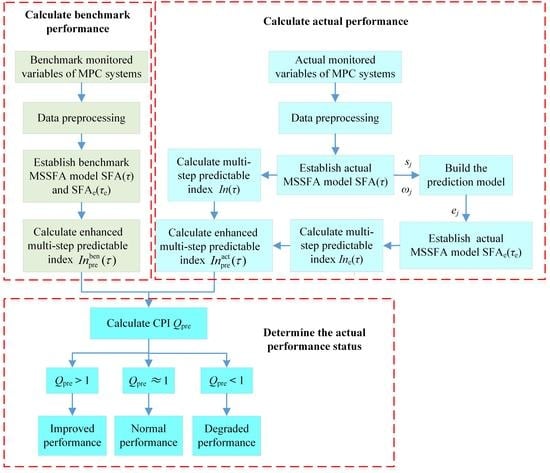
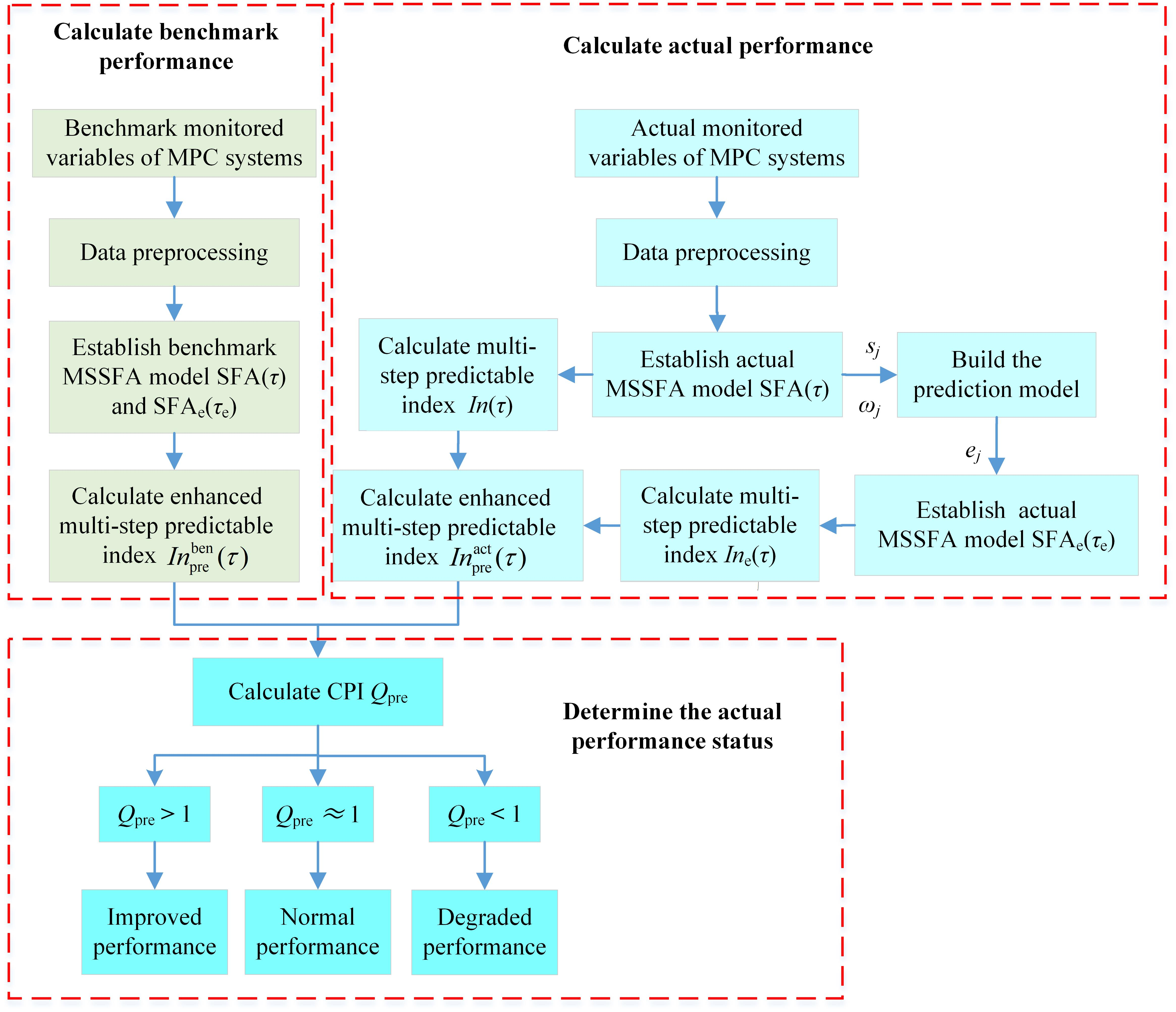
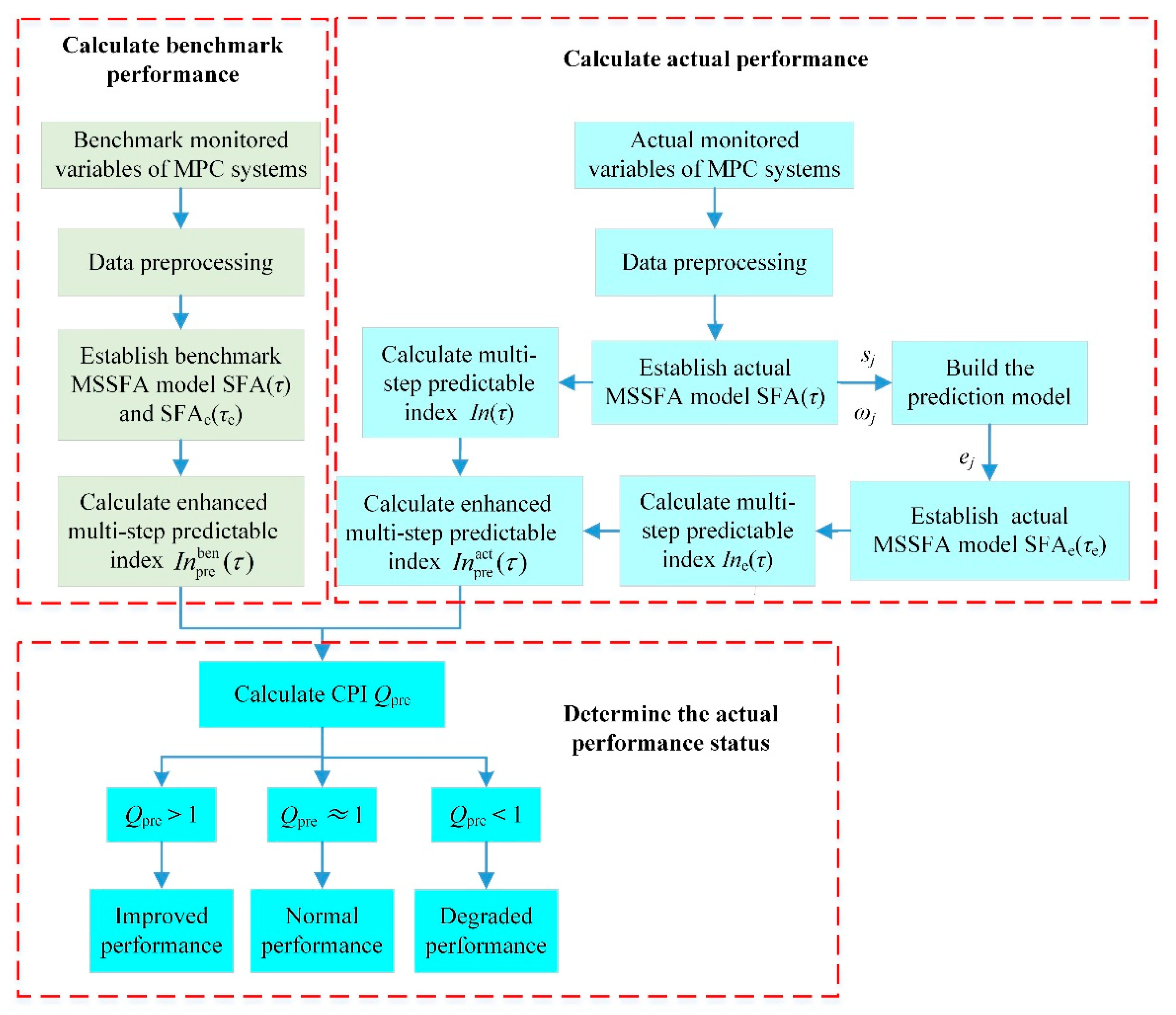
4. Performance Assessment Procedure of Enhanced Multi-Step Predictable Index Based on MSSFA

The proposed enhanced multi-step predictable index based on MSSFA method applied to MPC performance assessment including three parts: calculation of benchmark performance and actual performance, determination of actual performance status. The performance assessment flow chart as shown in Figure 4. Generally, benchmark data could be a period of “golden” operation data from the process data contained in the DCS database with satisfactory control performance. For example, the benchmark data could be a period of operation data after a satisfactory controller tuning or updating [26,28].

The performance assessment procedure can be described in detail as follows:

The calculation of benchmark performance:

(1)

The monitored variables when the MPC is in a good state are selected from the historical data contained in the DCS database for calculating the benchmark performance of the MPC.

(2)

Normalize the selected monitored variables so that the variable data is zero mean and unit variance.

(3)

Based on the benchmark monitored variables, build the MSSFA model SFA(τ) and SFA_e(τ_e) under benchmark performance using Equation (20).

(4)

Based on the MSSFA model, calculate the enhanced multi-step predictable index $I{n}_{\mathrm{pre}}^{\mathrm{ben}}(\tau )$ as the benchmark performance.

The calculation of actual performance:

(1)

Collect actual monitored variables $x_{\mathrm{act}}$ from the MPC system and built MSSFA model SFA(τ) under actual performance.

(2)

Calculate the multi-step predictable index $In(\tau )$ using Equation (22) and build the prediction model using Equation (23) to predict the SFs of SFA(τ).

(3)

According to the prediction error of the SFs, build MSSFA model SFA_e(τ_e) and calculate the corresponding multi-step predictable index $I{n}_{\mathrm{e}}^{}(\tau )$ using Equation (25).

(4)

Calculate the enhanced multi-step predictable index $I{n}_{\mathrm{pre}}^{\mathrm{act}}(\tau )$ using Equation (26) as the actual performance.

The determination of actual performance status:

(1)

Calculate the CPI $Q_{\mathrm{pre}}$ using Equation (27).

(2)

Determine the actual performance: if $Q_{\mathrm{pre}}>1$, the actual performance is improved relative to the selected benchmark performance; if $Q_{\mathrm{pre}}\approx 1$, the actual performance is equivalent to the selected benchmark performance; if $Q_{\mathrm{pre}}<1$, the actual performance is degraded relative to the selected benchmark performance.

5. Case Study

In this section, we demonstrate the results of the proposed multi-step predictable index with two processes. One is a numerical example [28,39], while the other is a continuous stirred tank heater (CSTH) simulation model, which is a benchmark model proposed by Thornhill et al. [42].

5.1. Numerical Example

A numerical example is given by [28,39]:

$$\mathit{y}(k)={\mathit{G}}_p\mathit{u}(k)+{\mathit{G}}_d\mathit{a}(k)$$

(28)

where

$${\mathit{G}}_p=\left[\begin{array}{cc}\frac{q^{-1}}{1-0.4q^{-1}}\hfill & \frac{K_{12}{q}^{-1}}{1-0.4q^{-1}}\hfill \\ \frac{0.3q^{-1}}{1-0.1q^{-1}}\hfill & \frac{q^{-2}}{1-0.8q^{-1}}\hfill \end{array}\right]$$

(29)

$${\mathit{G}}_d=\left[\begin{array}{cc}\frac{1}{1-0.5q^{-1}}\hfill & \frac{-0.6}{1-0.5q^{-1}}\hfill \\ \frac{0.5}{1-0.5q^{-1}}\hfill & \frac{1}{1-0.5q^{-1}}\hfill \end{array}\right]$$

(30)

are the process transfer function and disturbance transfer function, respectively; $q^{-1}$ is the backshift operator. The noise $\mathit{a}(k)$ follows a standard Gaussian distribution with the covariance ${\Sigma }_a=diag\{0.01,0.01\}$. $K_{12}$ is a constant parameter that can be resized to change the process model. When $K_{12}=0$, the MPC controller is designed and the MPC system operates under the optimal state. The parameters of the MPC controller are $P=20$, $M=1$, $\mathit{Q}=\mathit{I}$, and $\mathit{R}=0.1\mathit{I}$.

In this case, let $K_{12}$ increase from 0 to 10, which makes the MPC performance gradually deteriorate. 2000 samples are collected for establishing SFA(τ) and SFA_e(τ_e) models. When $K_{12}$ increases from 0 to 10, the trajectories of the slowness of the slowest SF under the SFA(τ) and SFA_e(τ_e) models are shown in Figure 5. In Figure 5, under the same $K_{12}$, as $\tau$ and ${\tau }_{\mathrm{e}}$ increase, the values of ${\omega }_{\min }^{}(\tau )$ and ${\omega }_{\min }^{\mathrm{e}}({\tau }_{\mathrm{e}})$ gradually approach the value 2, which implies that the extracted predictable information is getting less and less. When τ reaches a certain value $f$, the predictable information that can be extracted by the slowness is negligible, and the value of f can be selected as the truncation step.

The more predictable information in the monitored data, the higher its predictability, which means the poorer the MPC control performance. The predictable information can be measured by the distance between the value 2 and the slowness of the slowest SF. The smaller the distance, the lower the predictability, which means the better the control performance. From Figure 5a, it can be seen that when $\tau =1, 2 ,\cdots , 7$, the trajectories of ${\omega }_{\min }^{}(\tau )$ decrease significantly and get farther from the value 2. This means an increase in predictability. When $\tau =8, 9, 10$, the changes of the trajectories of ${\omega }_{\min }^{}(\tau )$ are not obvious and ${\omega }_{\min }^{}(\tau )$ are very close to 2. This means that predictability is low and does not change much. From Figure 5b, it can be seen that when ${\tau }_{\mathrm{e}}=1, 2, \cdots , 10$, the trajectories of ${\omega }_{\min }^{\mathrm{e}}({\tau }_{\mathrm{e}})$ decrease significantly and get away from the value 2. By comparing the trends of the trajectories of ${\omega }_{\min }^{}(\tau )$ and ${\omega }_{\min }^{\mathrm{e}}({\tau }_{\mathrm{e}})$, it can be seen that ${\omega }_{\min }^{\mathrm{e}}({\tau }_{\mathrm{e}})$ can further mine predictable information in monitored variables. In addition, the original one-step predictable index uses only ${\omega }_{\min }^{}(1)$ in Figure 5a to extract predictable information from the monitored variables. Obviously, the multi-step predictable index can more fully extract predictable information in the monitored variables by selecting the appropriate value of the truncation step f.

The multi-step predictable indices $In(\tau )$ and $I{n}_{\mathrm{pre}}^{}(\tau )$ are shown in Figure 6. It can be seen that as $\tau$ increases, $In(\tau )$ and $I{n}_{\mathrm{pre}}^{}(\tau )$ are closer and closer to the value 1, which means that the predictability is getting lower. This is consistent with the conclusion drawn from Figure 5. After $\tau$ increases to a certain value, the values of $In(\tau )$ and $I{n}_{\mathrm{pre}}^{}(\tau )$ change little and enter a stable area. A good choice for the truncation step of $\tau$ is just falling in this flat area [41]. In this example, the value of the truncation step $f$ is chosen as 20.

From Figure 6a, we can see that the traditional one-step predictable index is only displayed as a point in the solid blue box, while the multi-step predictable index is displayed as a performance trajectory. Therefore, the multi-step predictable index can provide more comprehensive assessment information. However, from the red dashed box in Figure 6a, it can be seen that there is some overlap between the performance trajectories under different $K_{12}$ values. That is, the sensitivity of the predictable index $In(\tau )$ is poor. In Figure 6b, as $K_{12}$ increases, the trajectories of predictable index $I{n}_{\mathrm{pre}}^{}(\tau )$ gradually move down. The MPC performance decreases along the direction of the arrow in Figure 6b, and it can tell the direction of performance changes. Compared with $In(\tau )$, the performance trajectories of $I{n}_{\mathrm{pre}}^{}(\tau )$ are separated from each other without overlapping. This indicates that the predictable index $I{n}_{\mathrm{pre}}^{}(\tau )$ is more sensitive to performance changes. In order to calculate the CPIs $Q$ and $Q_{\mathrm{pre}}$, we chose the MPC performance under $K_{12}=0$ as the benchmark performance. The results of the CPIs $Q$ and $Q_{\mathrm{pre}}$ are shown in

Table 1. Two CPIs under different $K_{12}$ values.

${\mathit{K}}_{12}$	0	2	4	6	8	10
$Q$	1.0000	0.9673	0.9307	0.9074	0.8888	0.8729
$Q_{\mathrm{pre}}$	1.0000	0.9316	0.8488	0.7963	0.7575	0.7268

. When $K_{12}$ increases, both $Q$ and $Q_{\mathrm{pre}}$ are less than 1, that is, both indices detect a performance deterioration. However, the value of the CPI $Q_{\mathrm{pre}}$ is smaller than that of the CPI $Q$ at the same $K_{12}$ value, and this confirms the above conclusion that $I{n}_{\mathrm{pre}}^{}(\tau )$ is more sensitive than In(τ).

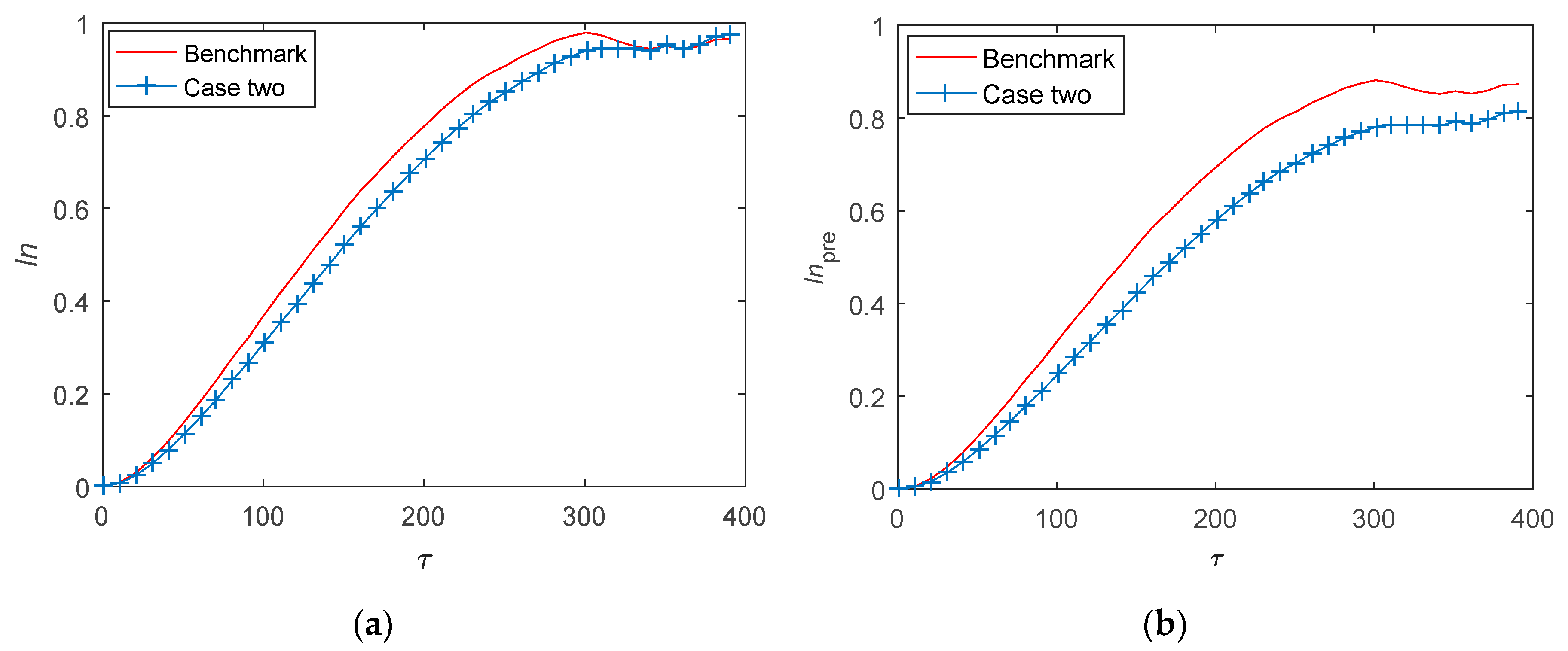
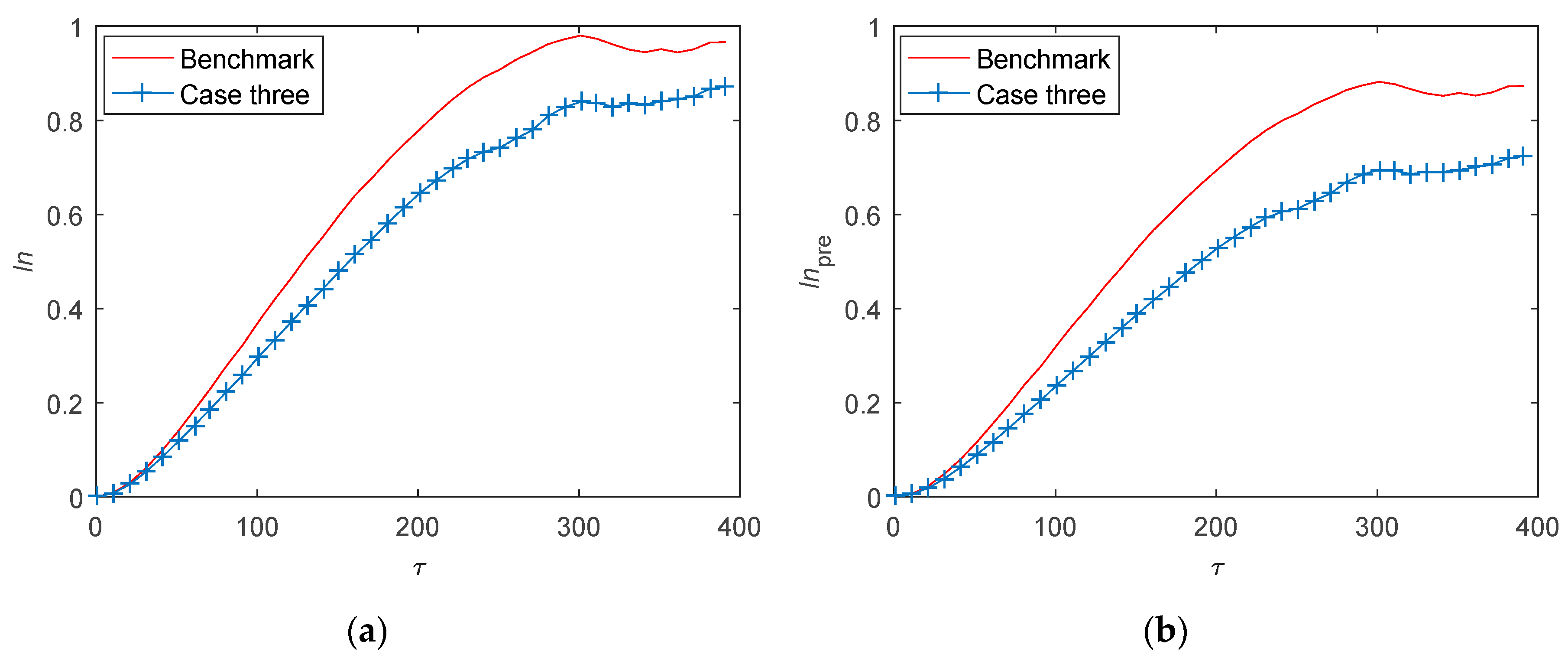
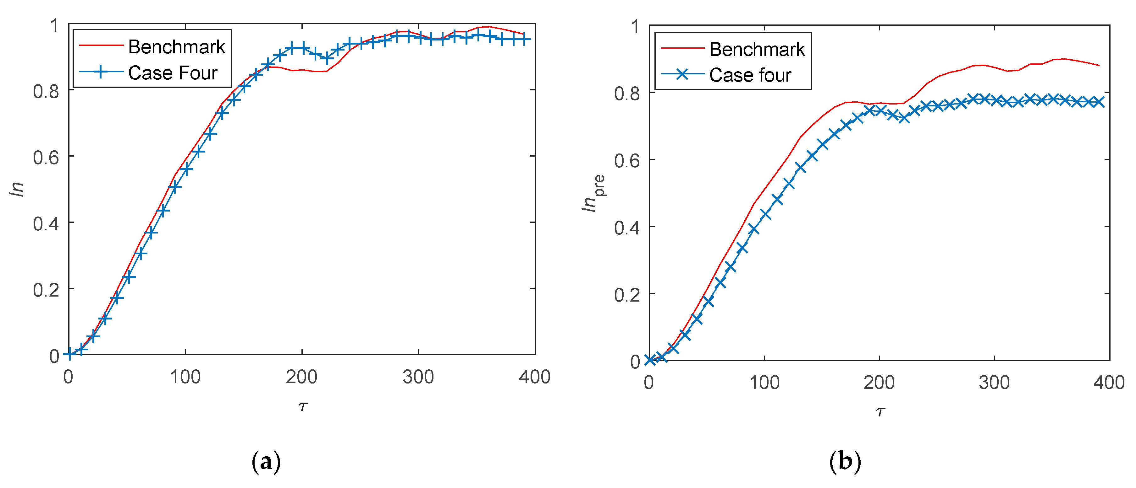
5.2. Continuous Stirred Tank Heater

In this section, the proposed multi-step predictable index is applied to a CSTH process, which is proposed by Thornhill et al. [42]. The CSTH is a hybrid simulation which uses measured data captured from a process to drive a first principles model. It has a complete characterization of the sensors and valves and the heat exchanger therefore have more complex and more realistic characteristics. Its structure is shown in Figure 7.

In CSTH, $u_1$ and $u_2$ are valve positions of the cold water and the steam in mA, respectively. $u_3$ and $u_4$ are valve positions of the hot water and the water outlet in mA, respectively. $y_1$ is the level measurement in mA and $y_3$ is the temperature measurement in mA. In the experiment, $u_1$ and $u_2$ are manipulated variables, $y_1$ and $y_3$ are controlled variables.

The dynamic volumetric and heat balances are shown below [42]:

$$\frac{dV(x)}{dt}=f_{\mathrm{cw}}+f_{\mathrm{hw}}-f_{\mathrm{out}}(x)$$

(31)

$$\frac{dH}{dt}=W_{\mathrm{st}}+h_{\mathrm{hw}}{\rho }_{\mathrm{hw}}{f}_{\mathrm{hw}}+h_{\mathrm{cw}}{\rho }_{\mathrm{cw}}{f}_{\mathrm{cw}}-h_{\mathrm{out}}{\rho }_{\mathrm{out}}{f}_{\mathrm{out}}(x)$$

(32)

where the parameters in the formula are described in

Table 2. Description of the parameters.

Parameter	Description	Parameter	Description
$x$	the level of water	$V$	the volume of water
$f_{\mathrm{cw}}$	the cold water flow into the tank	$f_{\mathrm{hw}}$	the hot water flow into the tank
$f_{\mathrm{out}}$	the outflow from the tank	$H$	the total enthalpy in the tank
$h_{\mathrm{hw}}$	the specific enthalpy of hot water feed	$h_{\mathrm{cw}}$	the specific enthalpy of cold water feed
${\rho }_{\mathrm{hw}}$	the density of incoming cold water	${\rho }_{\mathrm{cw}}$	the density of incoming hot water
${\rho }_{\mathrm{out}}$	the density of water leaving the tank	$W_{\mathrm{st}}$	the heat inflow from steam

. The operating condition of the CSTH system is shown in

Table 3. Operating condition of the continuous stirred tank heater system.

Variable	Operating Points
Level/cm	20.48
Cold water flow/cm3/s	90.38
Cold water valve/mA	12.96
Temperature/°C	42.52
Steam valve/mA	12.57
Hot water valve/mA	0
Hot water flow/cm3/s	0

.

The parameters of the MPC controller are $P=100$, $M=1$, $\mathit{Q}=\mathit{I}$, and $\mathit{R}=0.1\mathit{I}$. In order to study the effectiveness of the proposed multi-step predictable index for Gaussian distribution and non-Gaussian distribution, five different performance changes as shown in

Table 4. Parameter setting for performance changes.

Case	Parameter	Variation Range
Case one	Outlet flow	+1.4 cm3/s
Case two	Hot water flow	+0.3 cm3/s
Case three	Sensor bias in tank level	+1cm
Case four	Hot water flow	+0.6 cm3/s
Case five	Hot water flow	+0.6 cm3/s → +1.5 cm3/s

are designed. Among them, the noise in the first three cases follows the Gaussian distribution with standard deviation 0.03 and the noise in the other two cases follows the non-Gaussian distribution with standard deviation 0.03. 2000 samples under normal operating condition are collected to calculate the benchmark performance of the MPC system. According to the selection method of the truncation step, the value of $f$ is chosen as 400. The truncation step $f$ in the CSTH example is much larger than that in the numerical example. The reason can be derived from the autocorrelation plot of the four monitored variables the CSTH system, which is shown in Figure 8. From Figure 8, we can observe that $x_1$, $x_2$, and $x_3$ show higher autocorrelation, and the time lag is very large.

In case one, by changing the outlet valve $u_4$, the outlet flow increases by 1.4 cm³/s, which deteriorates the control performance. The performance assessment results are shown in Figure 9. In Figure 9a, when $\tau <116$, the trajectory of $In(\tau )$ is higher than the benchmark performance trajectory. This is inconsistent with the actual performance change. However, when $\tau >116$, the trajectory of $In(\tau )$ is lower than the benchmark performance trajectory. In Figure 9b, the trajectory of the proposed $I{n}_{\mathrm{pre}}^{}(\tau )$ is always lower than the trajectory of benchmark performance, that is, the performance degradation is completely detected.

In case two, by changing the valve $u_3$, the hot water flow increases by 0.3 cm³/s, which deteriorates the control performance. The performance assessment results are shown in Figure 10. From Figure 10a, it can be seen that when $\tau >350$, the trajectory of $In(\tau )$ is higher than the trajectory of benchmark performance. This is inconsistent with the actual performance change. In Figure 10b, the trajectory of the proposed $I{n}_{\mathrm{pre}}^{}(\tau )$ is always lower than the trajectory of benchmark performance and the performance degradation is completely detected.

In case three, the sensor of the tank level has a bias of 1 cm. The performance assessment results are shown in Figure 11. In Figure 11, the trajectories of $In(\tau )$ and $I{n}_{\mathrm{pre}}^{}(\tau )$ are significantly lower than that of the benchmark, indicating that both have detected a deterioration in performance. In addition, from the CPIs of $In(\tau )$ and $I{n}_{\mathrm{pre}}^{}(\tau )$ under case three in

Table 5. Two CPIs under different cases.

CPIs	Case One	Case Two	Case Three	Case Four
$Q$	0.9486	0.9018	0.8404	0.9706
$Q_{\mathrm{pre}}$	0.8425	0.8310	0.7720	0.8715

, it can be seen that the change of $I{n}_{\mathrm{pre}}^{}(\tau )$ is more obvious than that of In(τ).

In case four, process noise follows a uniform distribution with standard deviation 0.03. By changing the valve $u_3$, the hot water flow increases by 0.6 cm³/s. The performance assessment results are shown in Figure 12. In Figure 12a, the trajectory of $In(\tau )$ and the benchmark performance trajectory are very close, and when $166<\tau <250$, the trajectory of $In(\tau )$ is higher than the benchmark performance trajectory. In Figure 12b, the trajectory of the proposed $I{n}_{\mathrm{pre}}^{}(\tau )$ is always lower than the benchmark performance trajectory.

In case five, process noise follows a uniform distribution with standard deviation 0.03. By changing the valve $u_3$, and the hot water flow is gradually increased from 0.6 cm³/s to 1.5 cm³/s. The performance assessment results of $I{n}_{\mathrm{pre}}^{}(\tau )$ are shown in Figure 13. In Figure 13, as the hot water flow increases, the trajectories of $I{n}_{\mathrm{pre}}^{}(\tau )$ gradually move down. The direction of the arrow in Figure 13 indicates the direction of decline in MPC performance, and it can tell the direction of performance changes. Besides, from the results in case four and case five, it can be seen that the proposed index can effectively assess the deterioration of control performance under non-Gaussian distribution.

Two CPIs $Q$ and $Q_{\mathrm{pre}}$ under the first four cases are shown in Table 5. From Table 5 and the experimental results of the five cases, it can be seen that the proposed multi-step predictable index has better sensitivity to performance changes, can give the change direction of the MPC performance and be applied to both Gaussian and non-Gaussian distributions. It should be noted that the method proposed in this paper is suitable for linear time-invariant processes. It does not consider other characteristics of the process such as nonlinear, multi-mode and time-varying characteristics. The above characteristics of the process are also not considered in the case study. This will also be a problem that needs further research in the future.

6. Conclusions

Deterioration in MPC performance can lead to a decline in product quality and an increase in energy consumption. In this article, based on proposed MSSFA, an enhanced multi-step predictable index for evaluating the MPC performance is proposed. Due to the large time-delay that exists in the chemical industry process, there is considerable predictable information between the process variables with different step intervals. Compared with the traditional predictable index, the proposed method can effectively extract multi-step predictable information of monitored variables, and can better refine the predictable information in the process variables with a large lag. The experimental results demonstrate that the proposed CPA method provides a more-informative MPC performance assessment index, which can effectively indicate the direction of the performance change and improve the sensitivity to performance changes. Furthermore, the method is suitable for non-Gaussian distribution.

References

1. Xi, G.; Li, D.; Lin, S. Model predictive control—Status and challenges. Acta Autom. Sin. 2013, 39, 222–236. [Google Scholar] [CrossRef]
2. Qin, S.J.; Badgwell, T.A. A survey of industrial model predictive control technology. Control Eng. Pract. 2003, 11, 733–764. [Google Scholar] [CrossRef]
3. Tian, X.; Chen, G.; Chen, S. A data-based approach for multivariate model predictive control performance monitoring. Neurocomputing 2011, 74, 588–597. [Google Scholar] [CrossRef]
4. Zheng, Y.; Wei, Y.; Li, S. Coupling degree clustering-based distributed model predictive control network design. IEEE Trans. Autom. Sci. Eng. 2018, 15, 1749–1758. [Google Scholar] [CrossRef]
5. Jelali, M. Control Performance Management in Industrial Automation; Springer: London, UK, 2013. [Google Scholar]
6. Desborough, L. Increasing customer value of industrial control performance monitoring-Honeywell’s experience. In Proceedings of the Sixth International Conference on Chemical Process Control, Tucson, AZ, USA, 7–12 January 2001; p. 6. [Google Scholar]
7. Starr, K.D.; Petersen, H.; Bauer, M. Control loop performance monitoring—ABB’s experience over two decades. IFAC-PapersOnLine 2016, 49, 526–532. [Google Scholar] [CrossRef]
8. Schäfer, J.; Cinar, A. Multivariable MPC system performance assessment, monitoring, and diagnosis. J. Process Control 2004, 14, 113–129. [Google Scholar] [CrossRef]
9. Gao, X.; Yang, F.; Shang, C.; Huang, D. A review of control loop monitoring and diagnosis: Prospects of controller maintenance in big data era. Chin. J. Chem. Eng. 2016, 24, 952–962. [Google Scholar] [CrossRef]
10. Albarbar, A.; Arar, A. Performance Assessment and Improvement of Central Receivers Used for Solar Thermal Plants. Energies 2019, 12, 3079. [Google Scholar] [CrossRef]
11. Zhao, H.; Guo, S.; Zhao, H. Comprehensive performance assessment on various battery energy storage systems. Energies 2018, 11, 2841. [Google Scholar] [CrossRef]
12. Bauer, M.; Horch, A.; Xie, L.; Jelali, M.; Thornhill, N. The current state of control loop performance monitoring—A survey of application in industry. J. Process Control 2016, 38, 1–10. [Google Scholar] [CrossRef]
13. Grimble, M.J. Controller performance benchmarking and tuning using generalised minimum variance control. Automatica 2002, 38, 2111–2119. [Google Scholar] [CrossRef]
14. Huang, B. Multivariate Statistical Methods for Control Loop Performance Assessment. Ph.D. Thesis, University of Alberta, Edmonton, AB, Canada, 1998. [Google Scholar]
15. Julien, R.H.; Foley, M.W.; Cluett, W.R. Performance assessment using a model predictive control benchmark. J. Process Control 2004, 14, 441–456. [Google Scholar] [CrossRef]
16. Morari, M.; Lee, J.H. Model predictive control: Past, present and future. Comput. Chem. Eng. 1999, 23, 667–682. [Google Scholar] [CrossRef]
17. Zhang, Y.; Henson, M.A. A performance measure for constrained model predictive controllers. In Proceedings of the 1999 European Control Conference (ECC), Naples, Italy, 25–28 June 2019; pp. 918–923. [Google Scholar]
18. Patwardhan, R.S.; Shah, S.L.; Qi, K.Z. Assessing the performance of model predictive controllers. Can. J. Chem. Eng. 2002, 80, 954–966. [Google Scholar] [CrossRef]
19. Cai, L.; Thornhill, N.F.; Kuenzel, S.; Pal, B.C. Wide-area monitoring of power systems using principal component analysis and k-nearest neighbor analysis. IEEE Trans. Power Syst. 2018, 33, 4913–4923. [Google Scholar] [CrossRef]
20. Deng, X.; Tian, X.; Chen, S.; Harris, C.J. Nonlinear Process Fault Diagnosis Based on Serial Principal Component Analysis. IEEE Trans. Neural Netw. Learn. Syst. 2018, 29, 560–572. [Google Scholar] [CrossRef]
21. AlGhazzawi, A.; Lennox, B. Model predictive control monitoring using multivariate statistics. J. Process Control 2009, 19, 314–327. [Google Scholar] [CrossRef]
22. Shang, L.; Tian, X.; Cao, Y.; Cai, L. MPC performance monitoring and diagnosis based on dissimilarity analysis of pls cross-product matrix. Acta Autom. Sin. 2017, 43, 271–279. [Google Scholar]
23. Ge, Z. Review on data-driven modeling and monitoring for plant-wide industrial processes. Chemom. Intell. Lab. Syst. 2017, 171, 16–25. [Google Scholar] [CrossRef]
24. Zhang, Q.; Li, S. Performance monitoring and diagnosis of multivariable model predictive control using statistical analysis. Chin. J. Chem. Eng. 2006, 14, 207–215. [Google Scholar]
25. Zhao, S.J.; Zhang, J.; Xu, Y.M. Performance monitoring of processes with multiple operating modes through multiple PLS models. J. Process Control 2006, 16, 763–772. [Google Scholar] [CrossRef]
26. Yu, J.; Qin, S. Statistical MIMO controller performance monitoring. Part I: Datadriven covariance benchmark. J. Process Control 2008, 18, 277–296. [Google Scholar] [CrossRef]
27. Yu, J.; Qin, S. Statistical MIMO controller performance monitoring. Part II: Performance diagnosis. J. Process Control 2008, 18, 297–319. [Google Scholar] [CrossRef]
28. Li, C.; Huang, B.; Zheng, D.; Qian, F. Multi-input-multi-output (MIMO) control system performance monitoring based on dissimilarity analysis. Ind. Eng. Chem. Res. 2014, 53, 18226–18235. [Google Scholar] [CrossRef]
29. Yan, Z.; Chan, C.; Yao, Y. Multivariate control performance assessment and control system monitoring via hypothesis test on output covariance matrices. Ind. Eng. Chem. Res. 2015, 54, 5261–5272. [Google Scholar] [CrossRef]
30. Wu, P. Performance monitoring of MIMO control system using Kullback-Leibler divergence. Can. J. Chem. Eng. 2018, 96, 1559–1565. [Google Scholar] [CrossRef]
31. Xu, Y.; Zhang, G.; Li, N.; Zhang, J.; Li, S.; Wang, L. Data-driven performance monitoring for model predictive control using a mahalanobis distance based overall index. Asian J. Control 2019, 21, 891–907. [Google Scholar] [CrossRef]
32. Xu, Y.; Li, N.; Li, S. A Data-driven performance assessment approach for MPC using improved distance similarity factor. In Proceedings of the IEEE 10th Conference on Industrial Electronics and Applications (ICIEA), Auckland, New Zealand, 15–17 June 2015; pp. 1870–1875. [Google Scholar]
33. Shang, C.; Yang, F.; Gao, X.; Huang, X.; Johan, A.K.; Huang, D. Concurrent monitoring of operating condition deviations and process dynamics anomalies with slow feature analysis. AIChE J. 2015, 61, 3666–3682. [Google Scholar] [CrossRef]
34. Shang, C.; Huang, B.; Yang, F.; Huang, D. Slow feature analysis for monitoring and diagnosis of control performance. J. Process Control 2016, 39, 21–34. [Google Scholar] [CrossRef]
35. Zhang, H.; Tian, X.; Deng, X.; Cao, Y. Multiphase batch process with transitions monitoring based on global preserving statistics slow feature analysis. Neurocomputing 2018, 293, 64–86. [Google Scholar] [CrossRef]
36. Shang, C.; Huang, B.; Yang, F.; Huang, D. Probabilistic slow feature analysis-based representation learning from massive process data for soft sensor modeling. AIChE J. 2015, 61, 4126–4139. [Google Scholar] [CrossRef]
37. Zhao, H.; Zhao, C. Fine-scale online assessment of glycemic control performance based on temporal feature analysis. Ind. Eng. Chem. Res. 2019, 58, 4374–4386. [Google Scholar] [CrossRef]
38. Qin, Y.; Zhao, C. Comprehensive process decomposition for closed-loop process monitoring with quality-relevant slow feature analysis. J. Process Control 2019, 77, 141–154. [Google Scholar] [CrossRef]
39. Shang, L.; Wang, Y.; Deng, X.; Cao, Y.; Wang, P.; Wang, Y. A model predictive control performance monitoring and grading strategy based on improved slow feature analysis. IEEE Access 2019, 7, 50897–50911. [Google Scholar] [CrossRef]
40. Huang, B.; Ding, S.; Thornhill, N. Alternative solutions to multivariate control performance assessment problems. J. Process Control 2006, 16, 457–471. [Google Scholar] [CrossRef]
41. Thornhill, N.F.; Oettinger, M.; Fedenczuk, P. Refinery-wide control loop performance assessment. J. Process Control 1999, 9, 109–124. [Google Scholar] [CrossRef] [Green Version]
42. Thornhill, N.F.; Patwardhan, S.C.; Shah, S.L. A continuous stirred tank heater simulation model with applications. J. Process Control 2008, 18, 347–360. [Google Scholar] [CrossRef] [Green Version]
Figure 1. Graphical structure of the traditional slow feature analysis.
Energies 12 03799 g001
Figure 2. Graphical structure of the multi-step slow feature analysis.
Energies 12 03799 g002
Figure 3. Calculation flow chart of the enhanced multi-step predictable index.
Energies 12 03799 g003
Figure 4. The performance assessment flow chart of the multi-step predictable index based on multi-step slow feature analysis.
Energies 12 03799 g004
Figure 5. The trajectories of the slowness of the slowest SF: (a) the trajectories of ω min ( τ ) in SFA(τ), (b) the trajectories of ω min e ( τ e ) in SFAe(τe).
Energies 12 03799 g005
Figure 6. Performance assessment trajectories under different K 12 values: (a) multi-step predictable index of I n ( τ ) , (b) multi-step predictable index of I n pre ( τ ) .
Energies 12 03799 g006
Figure 7. The continuous stirred tank heater.
Energies 12 03799 g007
Figure 8. Autocorrelation plots for four monitored variables in the CSTH system.
Energies 12 03799 g008
Figure 9. Performance assessment trajectories under case one: (a) multi-step predictable index of I n ( τ ) , (b) multi-step predictable index of I n pre ( τ ) .
Energies 12 03799 g009
Figure 10. Performance assessment trajectories under case two: (a) multi-step predictable index of I n ( τ ) , (b) multi-step predictable index of I n pre ( τ ) .
Energies 12 03799 g010
Figure 11. Performance assessment trajectories under case three: (a) multi-step predictable index of I n ( τ ) , (b) multi-step predictable index of I n pre ( τ ) .
Energies 12 03799 g011
Figure 12. Performance assessment trajectories under case four: (a) multi-step predictable index of I n ( τ ) , (b) multi-step predictable index of I n pre ( τ ) .
Energies 12 03799 g012
Figure 13. Performance assessment trajectories of I n pre ( τ ) under case five.
Energies 12 03799 g013