1. Introduction
With the widespread popularity of GPS, smart phones and other location-aware devices, various kinds of location services and mobile social network applications continue to emerge, thus accumulating a large number of geographic location data, such as user check-in data, vehicle GPS trajectory, micro-blog, Twitter and other massive location data [
1]. Applications based on these location data have great application value in areas such as traffic management and control [
2], recommendation systems [
3], advertising [
4], public facility location and assessment, abnormal population identification and evacuation [
5]. Therefore, how to effectively and quickly mine meaningful potential patterns becomes the main challenge in processing location data.
The location data records the time and space trajectory information of the user, and embodies the change of the position of the moving object, such as the movement of the person, the movement of the vehicle, and the like [
6]. The location data in the city mainly comes from traffic vehicle trajectory data [
7], mobile communication location data, mobile social network check-in data [
8], mobile media location data, e-commerce logistics location information, and AFC(Automatic Fare Collection) location records [
9]. The analysis of massive location data can quantitatively describe and estimate people’s social activity characteristics, find people’s behavior patterns under different time and space granularities, gain insight into the overall movement trend of the group, and identify the routes and regions that people are interested in [
10,
11,
12]. Therefore, through the mining of location data can help people understand and discover the great value implied in location data. For example, literature [
13] discover relevant interest point patterns by mining users’ GPS trajectories, and then find popular tourist routes; literature [
14] also mine personal historical location data to realize user’s friend recommendation and scenic spot recommendation.
In the application of location data analysis and processing, clustering technology is often used to pre-process and analyze location data to discover spatial or temporal clustering patterns in location data [
15,
16]. There are many kinds of spatial clustering analysis algorithms, the specific selection depends on the type of data, clustering purposes and other aspects. At present, the commonly used spatial clustering algorithms can be roughly divided into the following five categories: partition-based clustering algorithm, hierarchical clustering algorithm, density-based clustering algorithm, grid-based clustering algorithm and model-based clustering algorithm [
17]. Because of the massive location data, arbitrary spatial distribution, fast update speed and large hybrid, density-based DBSCAN algorithm can find clusters of arbitrary shape, and can deal with noise. It is often used in pattern discovery of large location data [
18]. However, DBSCAN algorithm has some shortcomings, such as low processing speed when the amount of data is large, in addition, because the density distribution of location data is not uniform, it is difficult for DBSCAN algorithm to be applied in practice, so scholars have improved it in many aspects.
In order to solve the problem of parameter selection and global parameters of DBSCAN, OPTICS(Ordering Points to Identify the Clustering Structure) algorithm is proposed in the literature [
19], according to the concepts of core distance and accessible distance, ranks the objects in the data set and outputs an ordered list of objects. The information contained in the list of objects can be used to extract clustering, that is, classify the objects. Compared with the traditional clustering algorithm, the OPTICS algorithm has the greatest advantage that it does not depend on the input parameters. However, the algorithm does not produce clustering results visually, only by sorting the objects, and finally gives an extended cluster sorting structure interactively. DMDBSCAN algorithm [
20] is similar to VDBSCAN (Varied Density DBSCAN) algorithm [
21], which is an improved clustering algorithm for non-uniform data sets. By sorting and visualizing the parameter
values of the objects in the data set, can observe the key points of drastic changes in the
sorting graph to divide the non-uniform data set into density levels. However, the two algorithms can not automatically segment and extract the density hierarchy of data sets. The algorithm SA-DBSCAN(Self-adaptive DBSCAN) [
22] fits the parameter
curve by inverse Gauss function according to the statistical characteristics of the data set, and automatically determines the global density parameters, which greatly reduces the dependence of DBSCAN on parameters. However, when clustering data sets with non-uniform density, the clustering effect of SA-DBSCAN algorithm will be greatly disturbed. DBSCAN algorithm has a high I/O overhead when the amount of data is large, which leads to low clustering efficiency. Many scholars have proposed corresponding improved algorithms to improve its efficiency. In order to extend to large-scale data clustering, a common method is to prune the search space of neighborhood queries in DBSCAN using spatial indexing technology (such as R-Tree) to improve clustering efficiency, but the efficiency of optimization algorithm still depends on data size [
23]. A density clustering algorithm DBCURE-MR based on MapReduce is proposed in the literature [
24]. Although the method achieves speedup of more than ten times or tens of times, it needs the support of dedicated processors or clusters of dedicated servers.
In this paper, a fast hierarchical clustering algorithm based on Gaussian mixture model is proposed for the rapid clustering problem of location data with uneven density distribution. The Gaussian mixture model based on DBSCAN algorithm can realize the density aggregation of position data in general computing platform. First, the Gaussian mixture model is used to fit the probability distribution of the dataset to determine different density levels; then, based on the DBSCAN algorithm, the sub-datasets with different density levels are locally clustered, and at the same time, the appropriate seeds are selected to complete the cluster expansion; finally, the sub-datasets clustering results are merged. In the method clustering effect analysis, multi-angle experimental evaluations were performed on multiple public test data and large-scale location data (from Microsoft T-Driver project) to verify the clustering effect and performance of the proposed algorithm. The method is applied to the identification of the distribution of passenger flow clusters by using the peak time data of the actual urban rail station.
The structure of this paper is as follows:
Section 2 describes the core idea and detailed process of the improved DBSCAN algorithm. In
Section 3, multi-angle (accuracy, noise impact, time efficiency) experimental evaluations were carried out on multiple public test data and large-scale location data (Microsoft T-Driver project) to verify the clustering effect of the proposed algorithm. In
Section 4, the improved algorithm is applied to the recognition of passenger gathering characteristics in urban rail transit stations.
Section 5 concludes the paper.
2. Improved DBSCAN Algorithm for Heterogeneous Data
For the location data set with uneven density distribution, the basic idea of the algorithm is as follows: firstly, Gauss mixture model is used to obtain the density and distribution characteristics of location data set, so as to realize the hierarchical processing of non-uniform density data set; then, a fast expansion processing method of data cluster is designed to improve DBSCAN algorithm and realize clustering analysis of hierarchical data sets. The core idea of the algorithm is as follows: (1) hierarchical processing for data sets with uneven density distribution; (2) fast cluster expansion processing.
2.1. Symbolic Description
For the convenience of understanding the method, the relevant parameters are shown in
Table 1.
2.2. Density Layering Based on Gauss Mixture Model
The distribution characteristics of sample points in data set are fitted by a linear combination of a certain number of Gauss distributions [
25,
26,
27]. The probability density function of each Gauss distribution is obtained by the expectation maximization algorithm (EM), and the probability density function is calculated for different sample points, to measure the density distribution of the sample point. The sample points with similar probability density function values are divided into the same density layer, so as to achieve stratified processing of uneven density data sets.
In the above process, the estimation of the unknown parameters in the Gaussian mixture model is the core of the dataset hierarchy. The author uses EM algorithm to solve the model parameters.
The form of the probability density function of the Gaussian mixture model [
28,
29] used in this paper is shown in Equations (
1) and (
2).
Among them: ,, is the expectation of the i-th Gaussian distribution, is the i-th gaussian distributed covariance matrix, m is the order of the Gaussian mixture model, d is the dimension of the vector.
The specific steps for estimating the parameters of the Gaussian mixture model using the EM algorithm are as follows, through the cycle E-Step, M-Step until the final result converges.
(E-Step) Calculate the value of the implicit variable from the value of the parameter estimated in the previous step:
(M-Step) Estimating the unknown parameter value according to the value of the implied variable:
When using the EM algorithm to solve Gaussian mixture model parameters, E-Step first uses the , , parameter values obtained by initializing M-Step to estimate the value of the implicit class variable ; then, the value is substituted into each formula of M-Step. The value of each , , parameter is calculated; when the maximum likelihood maximum value is obtained, the value needs to be recalculated, and iterates until the parameter estimation value obtained twice in succession satisfies the convergence condition of the algorithm and the algorithm terminates.
2.3. Parameter Determination of Data Sets with Different Density Levels
The dataset layered by the Gaussian mixture model eliminates the influence of uneven distribution of dataset density on the clustering effect. The traditional DBSCAN algorithm can be used to perform local clustering on the data set and obtain the appropriate and parameter values.
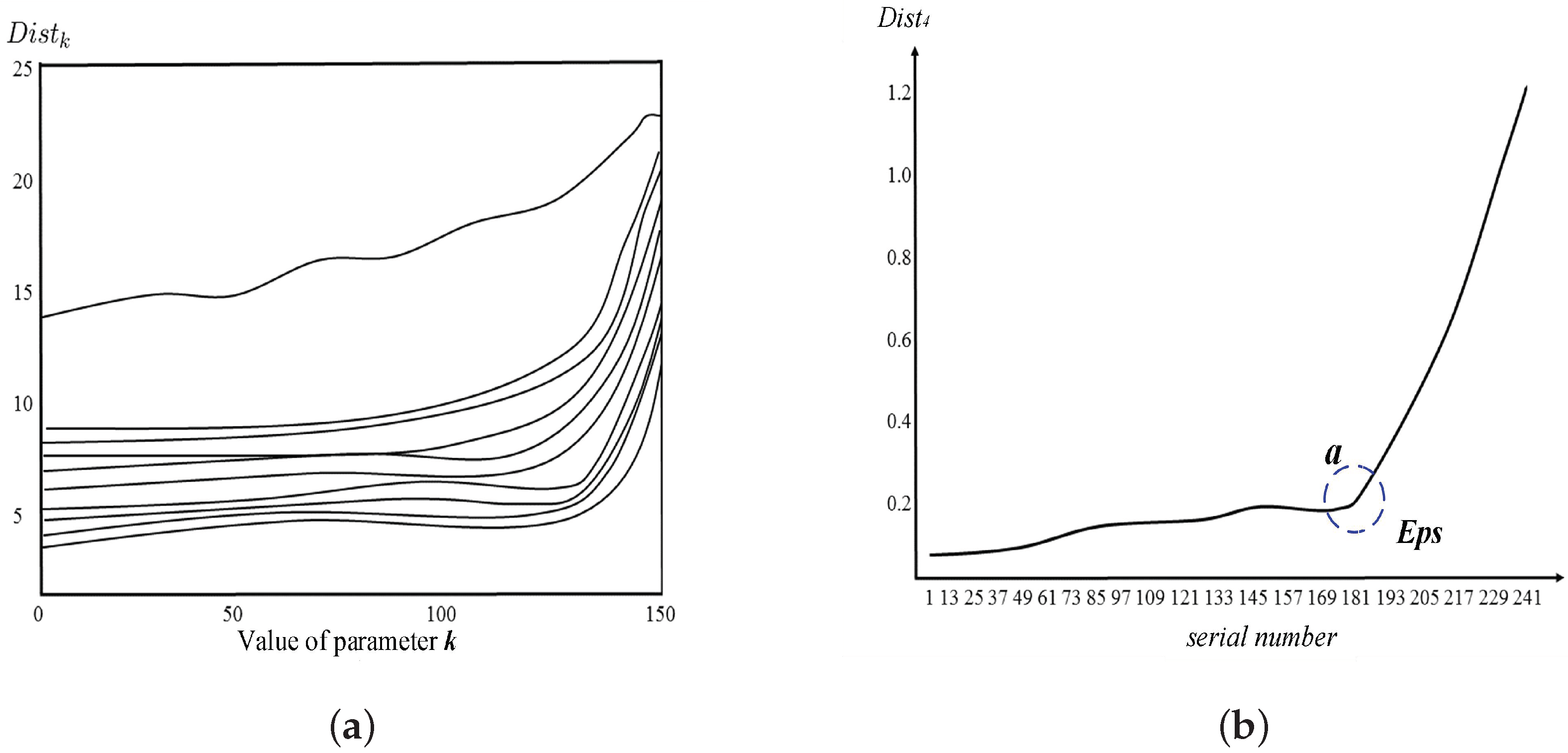
In the traditional DBSCAN algorithm, the threshold parameter
is usually set empirically; the value of the neighborhood radius
parameter is determined by traversing the distance between each sample point and all objects in the data set. That is, in the data set of a certain density layer, the
k-th nearest neighbor distance
is calculated for any sample point, and the distance values are sorted in ascending order. When the threshold parameter
value corresponds to multiple
k values, it can be obtained as shown in
Figure 1a. The distribution effect of
is shown;
Figure 1b shows the distribution of
for each sample point when the threshold parameter
.
It can be seen from
Figure 1 that the parallel distribution features of the density distribution curve of the dataset after dividing the hierarchy are obvious. In addition, most curves will have a turning point.
Figure 1 can reveal the density distribution characteristics of the dataset to some extent. In general, noise points and clusters in the dataset should have large density differences. That is, there is a certain threshold point in the
graph. The points in the dataset can be divided into two parts with large differences in density. This point is shown in
Figure 1b, which is a sudden change point of
curve from slow to steep
a. The characteristic of the mutation point is that the
k nearest neighbor distance
changes smaller before the point of mutation, and the
k nearest neighbor distance
of each sample point is larger after the mutation point
k. The data point on the right of the a point is the noise point of the low density distribution. The data point on the left of the
a point is the data point of the high density distribution, and the value
of the a point is
of the density parameter of the cluster, which is the value of the density parameter
. According to this feature, the
value corresponding to this point can be taken as the value of the
, that is, a set of maximum-density connected objects based on density re achability can be obtained. Through this method, the
parameter determination for a uniform density data set has better feasibility and effectiveness, and the processing process is relatively simple and rapid.
2.4. Fast Expansion of Clusters
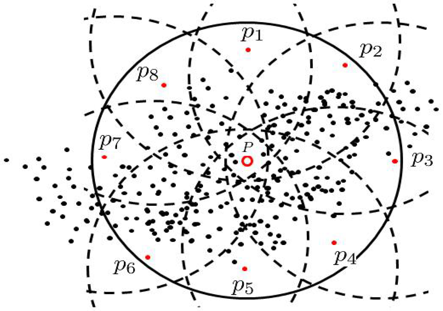
In view of the shortcomings of the traditional DBSCAN algorithm in the efficiency of execution, a Fast-DBSCAN algorithm is proposed. In the process of clustering the hierarchical data sets, all the density reachable objects in the neighborhood are classified as the same cluster, and then a certain number of representative points are selected as the seed objects to extend the cluster.When the number of seed objects is small, the algorithm will lose the object in the cluster expansion process. In this paper, 8 position points are taken as reference to select the representative points as seed objects when the two or more cluster extensions are extended, and there are usually
quadrants and
1 reference points for
N dimensional space, so the number of seed objects is up to
1. This paper focuses on the expansion of clusters in two-dimensional space, so it is reasonable to select 8 seed objects for arbitrary core objects. The selection method is to take the core object
p as the center, draw the circle with its
radius, first select 4 points at the top, the bottom, the left and the right of the circle, and then take the middle point of the arc between every two points of the above 4 points as the other 4 points, as shown in
Figure 2.
In the Algorithm 1, when the first core point of the new class is found, the first batch of representative points is selected as the seed point for class expansion. In the subsequent class expansion round, the new seed is continuously added to the seed point collection seed for subsequent class expansion. This cycle continues until the representative seed is empty. This indicates that the class has been expanded.
In the process ExpandCluster, a process Representative-Seed-Selection is added to select a representative point from the neighborhood of the core point.
| Algorithm 1 ExpandCluster (SetofPoints, , , ) |
Input: Data set D(Setofpoints), , ,
Output: Result of Cluster expansion
- 1:
for i=1 to Set of points-size do Point=Setofpoints.get(i) - 2:
if Point.ClusterID=Unclassified then - 3:
if ExpandCluster(SetofPoints, , , ) then - 4:
ClusterID=nextID(ClusterID) - 5:
end if - 6:
end if - 7:
end for - 8:
candidate.seeds=SetofPoints.query(Point,) - 9:
if candidate.seeds< then - 10:
SetofPoints.changeClusterID(Point,Noise); - 11:
return False; - 12:
else - 13:
SetofPoints.changeClusterID(candidate.seeds,ClusterID); - 14:
while ≠∅ do - 15:
current p=; - 16:
Result=SetofPoints.query(current p,); - 17:
if Result.size ≥ then - 18:
Rrepresentative.Seeds.Select (Result, , current p); - 19:
for each point p in Rrepresentative.Seeds do - 20:
if p. ClusterID= Unclassified then - 21:
Add point p to the set Rrepresentative.Seeds(); - 22:
end if - 23:
end for - 24:
else - 25:
for each point p in Result do - 26:
if p. ClusterID= Unclassified or Noise then - 27:
SetofPoints.changeClusterID(p,ClusterID); - 28:
end if - 29:
end for - 30:
end if - 31:
end while - 32:
Rrepresentative-Seeds.delete(current point p) - 33:
end if - 34:
return True.
|
2.5. Improved DBSCAN Algorithm for Heterogeneous Dataset
The input of the DBSCAN algorithm based on the Gaussian mixture model is the data set
D, the order
m of the Gaussian mixture model and the initial value of the parameter, and the threshold parameter
; the output is the cluster or cluster obtained by clustering. The flow of the algorithm is shown in
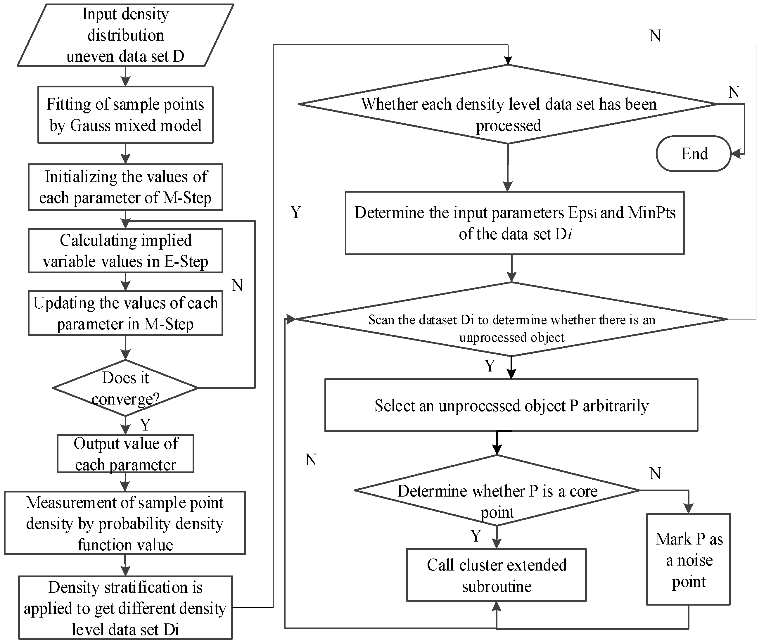
Figure 3, the pseudocode of the improved algorithm is shown in Algorithm 2.
Step 1: Determine the data set D, initialize the object, and mark the sample point as uncategorized.
Step 2: The Gauss mixture model is used to fit the sample points in the dataset D, and the EM model is used to solve the model parameters.
Step 3: The Gauss mixed model is represented as a linear combination of multiple Gauss distributions. Based on the value of the probability density function of each sample point, the data set of the density distribution is layered, and the data sets of different density levels, are obtained.
Step 4: According to the data set of different density levels, the threshold parameter is set to determine the value of parameters, and the local clustering of the data set is used in turn by using the traditional DBSCAN algorithm.
Step 5: Randomly select an unprocessed object p in the data set to find the total number of objects whose and density can reach, and determine the relationship between the number and the size of the . If the value is greater than or equal to the value of , consider p as the core. In this case, all the reachable objects in the neighborhood of p are grouped into a cluster. Step 6 is used to expand the cluster until no cluster can be added to the cluster. This clustering of the core object p is completed. If less than , p is marked as noise point, after the object p is processed, Step 5 is repeated until there is no unprocessed point in the data set . At this time, the data set of the density level has been clustered and transferred to the next density-level datasets are analyzed.
Step 6: Select k representative objects as seeds in the cluster to join . Determine whether the seed object in the is the core point. If it is not the core point, remove it directly from the . If it is the core point, then add the neighbors. The unclassified objects in the domain join the cluster, and continue to select representative objects as seeds in the neighborhood to join the . Then the seed objects in the are traversed, and uncategorized seeds are added to the as new seed objects. is now processed and removed from . The above process is repeated until all the seed objects in the are processed. At this time, the cluster expansion of the core point p ends, and the cluster expansion process of the next core point is transferred.
Step 7: When all the density level data sets are clustered, the clustering results of each data set can be merged to output the final clustering results of the whole data set D.
4. Cluster Analysis of Passenger Position Data in Urban Rail Stations
In this section, the simulation shows that the passenger flow position data has uneven distribution characteristics, and then the method validity is verified by using the peak time data of the actual platform.
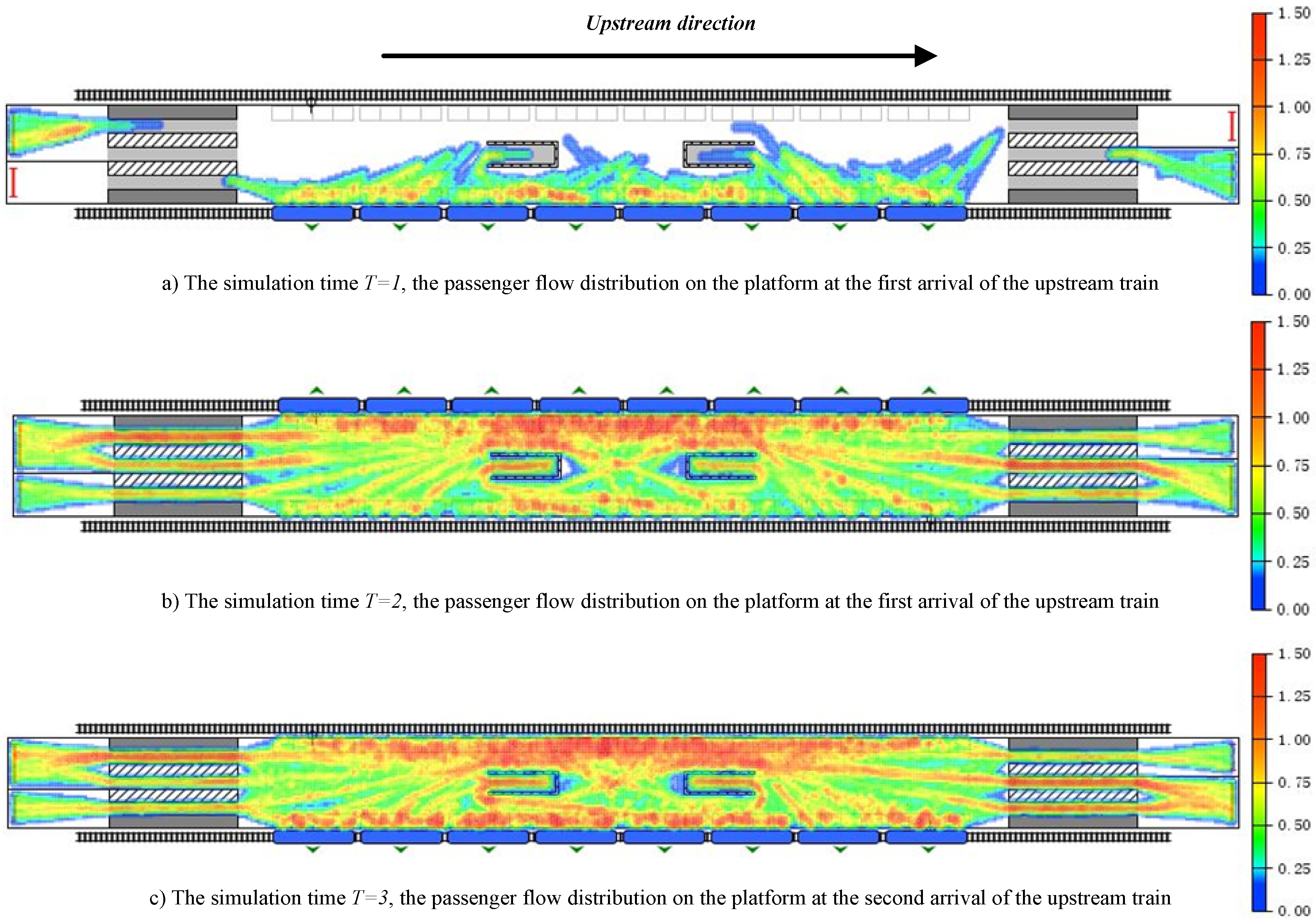
4.1. Uneven Distribution of Passenger Position Data
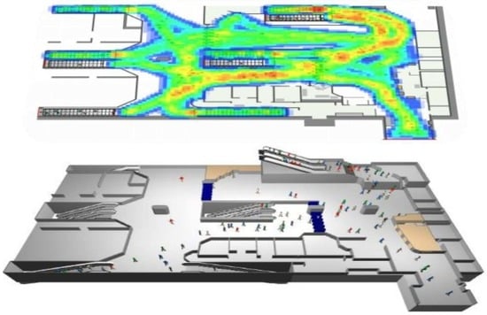
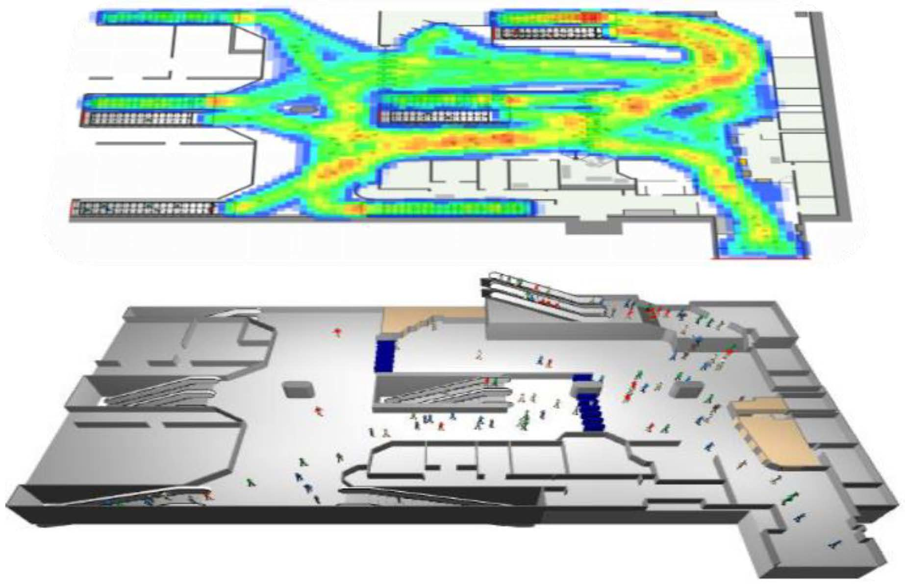
Cross-interference between passenger streamlines will lead to uneven density distribution of passenger groups in the station. On the basis of field investigation and simulation by Anylogic, the location distribution map of passenger groups at different times on the platform can be obtained. The simulation model of Anylogic in this paper is mainly divided into four modules: pedestrian behavior logic module, train logic module, Guo Gongzhuang platform physical environment module. In the pedestrian behavior logic module, pedestrian behavior logic module is constructed from two aspects: inbound passenger flow and outbound passenger flow. Part of the passenger flow goes directly to the platform for waiting, while the other part leaves the platform through stairway. When the train arrives and the waiting passengers finish boarding, the passenger flow disappears. The train logic module mainly simulates the process of subway train entering and leaving the station through Rail Libraiy. The module functions include the generation and disappearance of the train, the alighting of passengers and the boarding of waiting passengers after the arrival of the train. The physical environment module of the station includes the key facilities such as the wall, obstacles and stairs of the station. It is constructed with space marking tools in the pedestrian database. The parameters in the simulation are derived from the field investigation of Guogongzhuang Station on 23 July 2019. During peak hours, the departure interval of adjacent trains is about 150 s, and the average time of train stopover is 55 s. The ratio of passenger flow from left and right entrance to opposite platform is about 8.7:1.3 and 8.4:1.6. It can be seen that there is a more obvious non-uniform density distribution characteristic, as shown in
Figure 10.
In order to further verify the practicability of the proposed algorithm, the actual data of an urban rail transit station in Beijing was used to perform clustering analysis using the traditional DBSCAN algorithm and the proposed algorithm. The data of 18:00–18:30 in the evening peak period of Guogongzhuang subway station on 18 July 2016 is used as experimental data to investigate the performance and accuracy of the clustering algorithm. The data sample has a total of 50,000 sampling points.
Table 4 shows the information of each attribute data of some sampling points. Each sample point consists of attributes such as ID, time, longitude, and latitude. The data source is the passenger position data that is continuously uploaded to the database server in a fixed period (10 s) during the test of the WIFI positioning system in the transfer station.
The first column in the table is the data number, the second column is the mobile device (or passenger) number, the third column shows the time of data acquisition, and the fourth and fifth columns record the geographical coordinates of the passenger at that time.
4.2. Cluster Analysis of Passenger Position Data Based on Traditional DBSCAN Algorithm
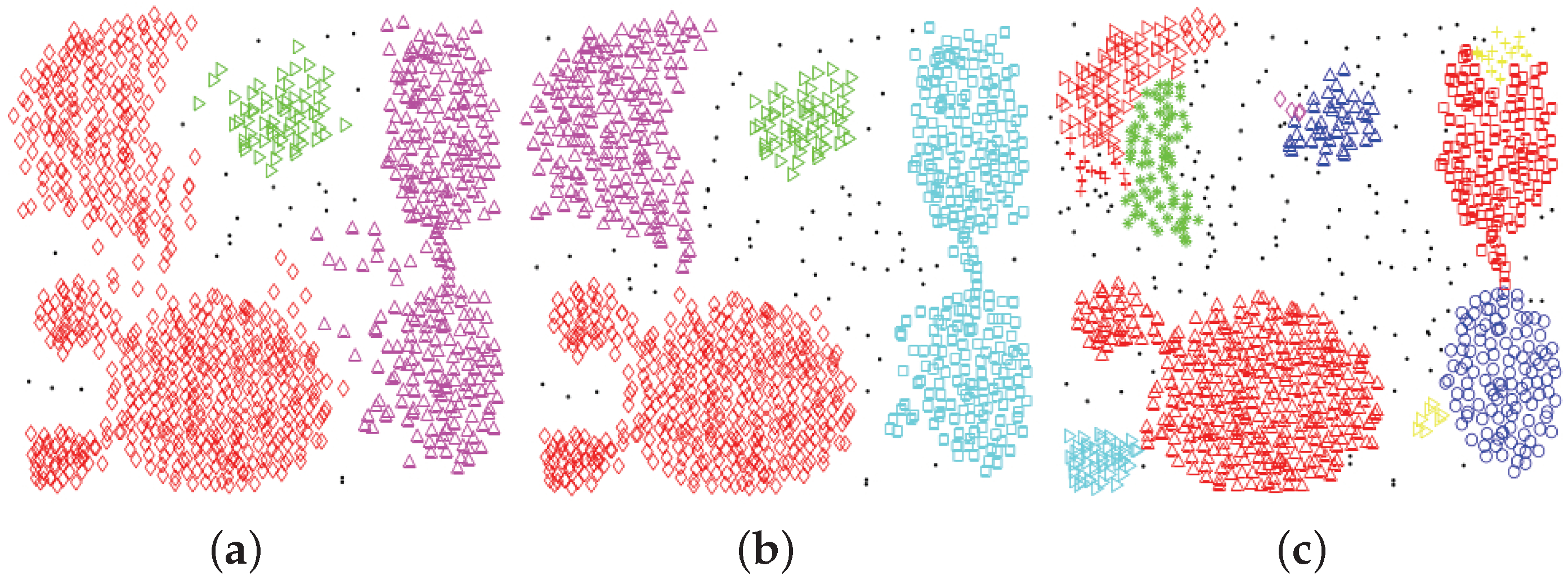
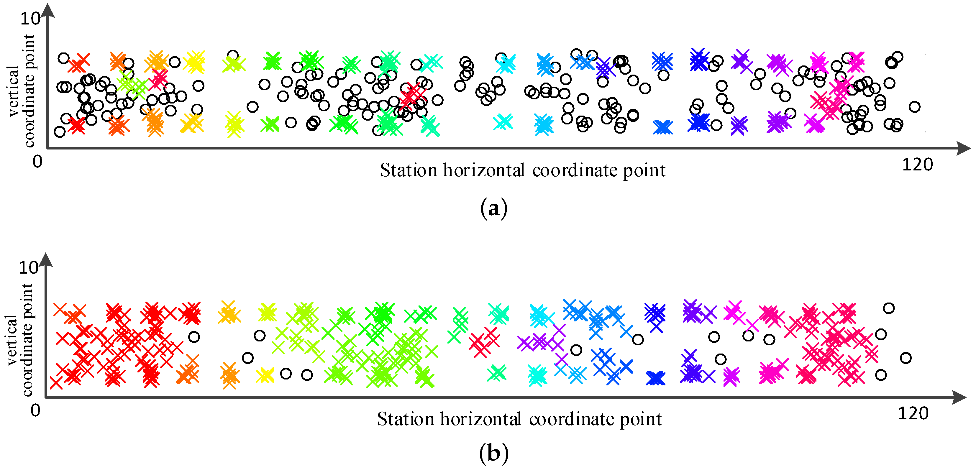
The traditional DBSCAN algorithm is used to perform cluster analysis on the above-mentioned passenger position data. The threshold parameter is set to 4, and different clustering effects can be obtained by selecting different values. The x of different colors in the figure represents different categories. o represents the noise point.
When
, the clustering effect of the algorithm is shown in
Figure 11a. Only the cluster analysis of high-density passenger position data can be achieved, but for low-density passenger position data, it is basically impossible to complete. Clustering results in a large number of passenger position data being treated as noise points, and it is not possible to present the aggregation and distribution characteristics of passenger mass transfer behavior.
When
, the clustering effect of the algorithm is shown in
Figure 11b, which can satisfy the cluster analysis of low-density distribution of passenger position data. However, because the value of the neighborhood parameter
is too large, it cannot correctly identifying the clustering and distribution characteristics of passenger clusters in similar areas results in the high density distribution of passenger location data being clustered into the same category.
It can be seen that using the traditional DBSCAN algorithm, cluster analysis is performed on the passenger position data with uneven density distribution. If the global parameter value is selected by referring to the high-density passenger position data, the low-density passenger position data cannot be clustered, and a large number of noise points are generated. If the global parameter value is selected by referring to the low-density passenger position data, the high-density passenger position data will be merged into the same cluster, which affects the accuracy of the clustering result.
4.3. Cluster Analysis of Passenger Position Data Based on Improved DBSCAN Algorithm
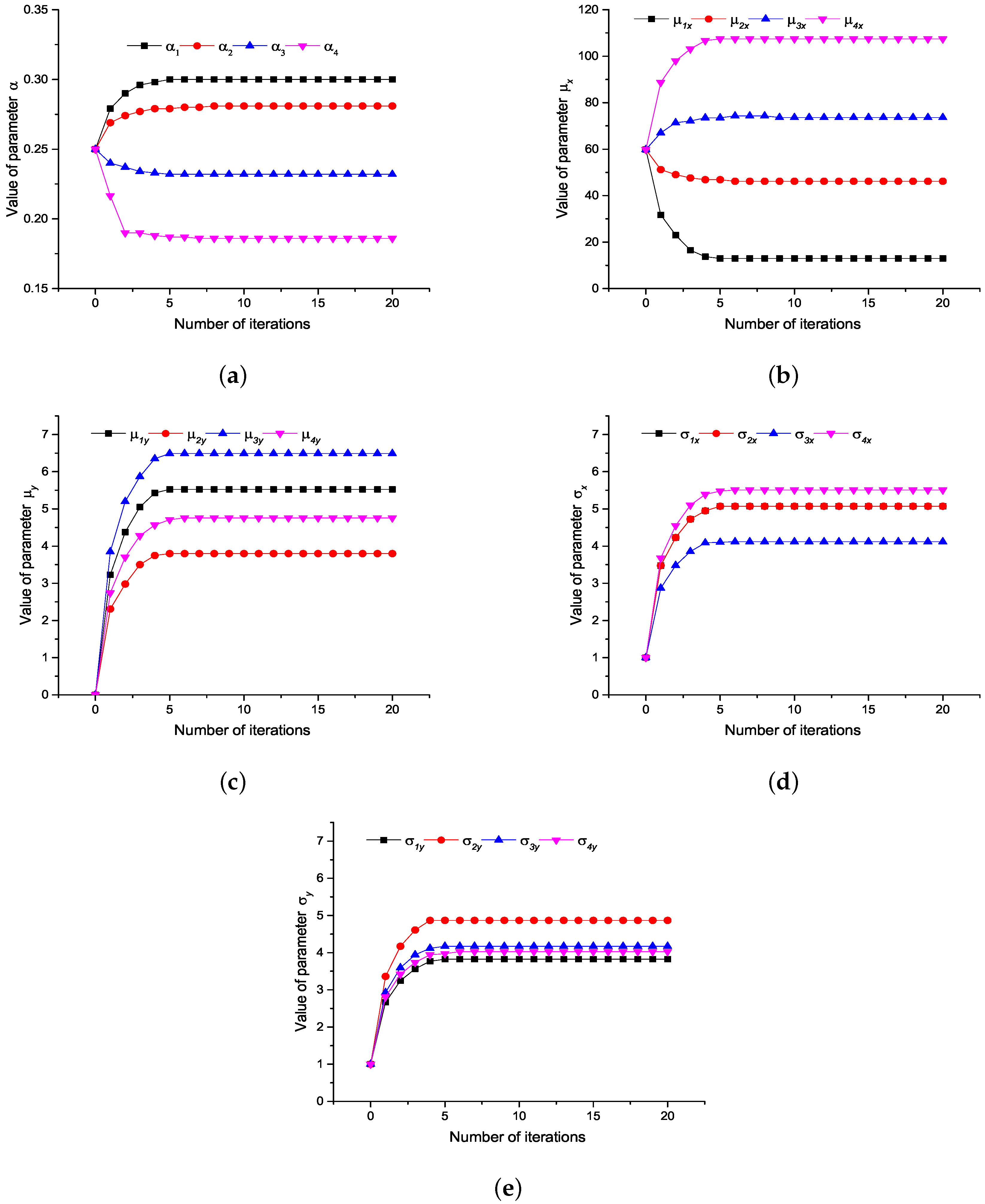
Using the DBSCAN algorithm based on the Gaussian mixture model proposed in this paper, the clustering test is conducted for the above dataset. The Gaussian mixture model was used to fit the test passenger position data set, and the model order was set to
. The probability density function formula was obtained from Equations (
1) and (
2) to fit the distribution of the passenger position data set on the platform at the moment. feature. In the fitting process, the EM algorithm parameters given in
Table 1 are used to solve the process, and the unknown parameter
in the Gaussian mixture model is estimated. The estimated results of each parameter are shown in
Table 5.
The location of the passenger’s location determines the range of the mean value of the single Gauss distribution to a certain extent, and the point of the passenger location data is fitted to the corresponding single Gauss distribution, while the remaining test passenger location data is fitted to the most suitable single Gauss distribution.
Figure 12 shows the iterative process that the parameters of the Gauss model are gradually convergent and stable.
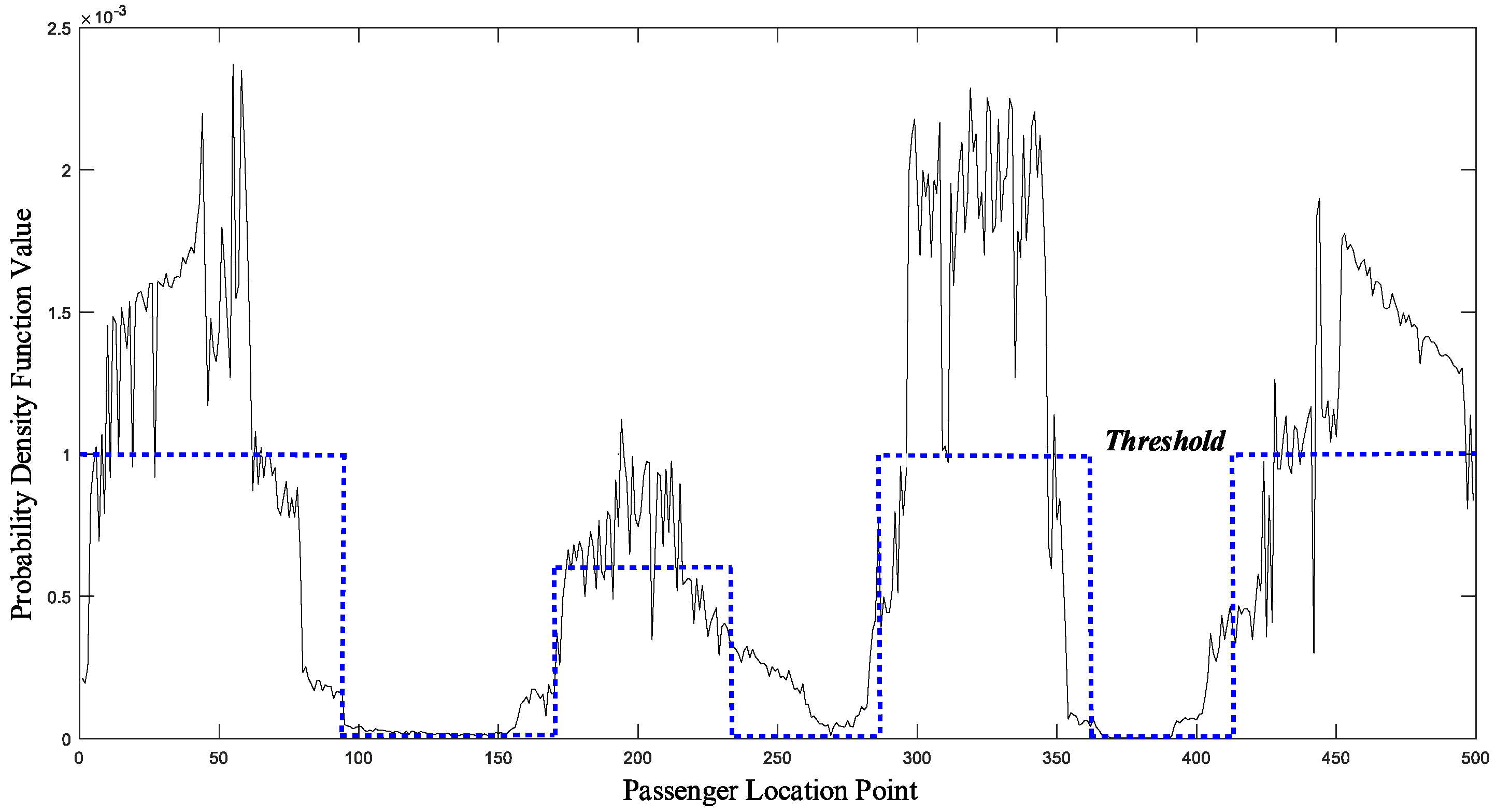
By setting the appropriate threshold and dividing the data set, we can get the hierarchical result for the dataset, as shown in
Figure 13.
According to the parameter determination method of the single density hierarchical data set, the clustering parameters of the first density data of the data concentration are
, and the clustering parameters of the second density hierarchical data are
. According to the order from small to large, the clustering is carried out in order, the higher density level of passenger location data is first clustered, and then the data of the lower density level are clustered, and the cluster is labeled as
(the
j cluster of the density level is
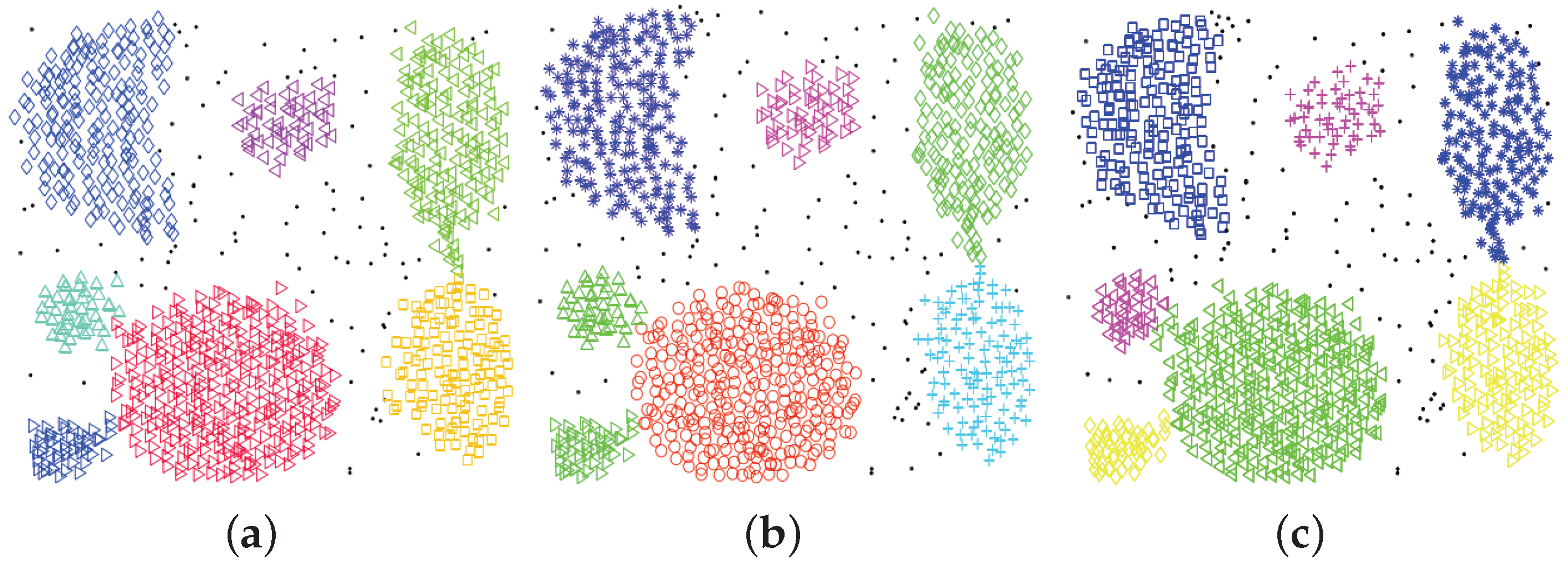
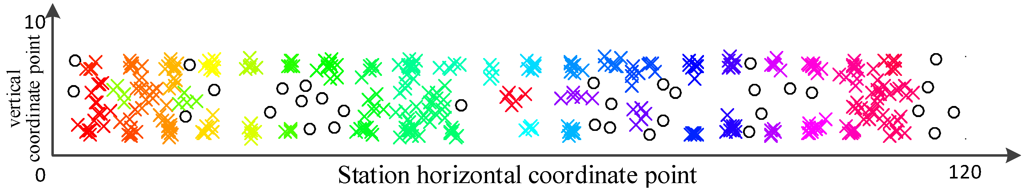
) so as to ensure that the sample points completing the clustering will not be repeated again. When the data of all density levels are clustered, the data points that are not clustered are labeled as noise points. With the local clustering results of different density level data, the aggregation and distribution characteristics of the passenger group behavior on the station platform can be obtained, as shown in
Figure 14.
Compared with the clustering results shown in
Figure 11a,b, the improved algorithm has a better clustering effect for high density distribution and low density distribution of passenger location data. At the same time, a large number of passenger location data are avoided to be mishandled as noise points, thus overcoming the defects of the traditional algorithm for the failure of the passenger cluster in the similar areas.
4.4. Passenger Location Aggregation Visualization
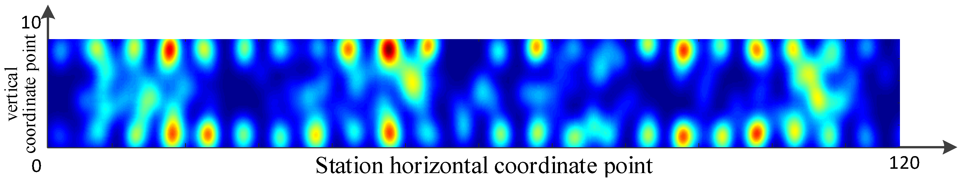
In order to intuitively describe the differences in the number, size, and degree of density between different passenger clusters, visualization of the heat map is used to present the aggregation and distribution characteristics of the passenger groups so as to facilitate the operator’s organization of the passengers and the evacuation of abnormal passenger flows. By establishing a reasonable mapping relationship between the passenger cluster characteristics and the visualization object, the discrete parameters of the passenger cluster are converted into a continuous form, and the passenger position data distribution characteristics are transmitted using the color change.
First, the passenger cluster space coordinates are projected to the interface coordinates, and the average of the coordinates of each passenger location in the cluster is worth the centroid of the map. The appropriate icon size is set by the envelope area method, so that it can truly reflect the range of the passenger cluster activity, and the passenger cluster is characterized by setting the color coverage range. In order to describe the difference between the density of the different passenger clusters and standardize the maximum density of the density, the degree of the aggregation of the passenger cluster is expressed by the linear gradient color, so as to ensure the fast and accurate identification of the passenger cluster with different distribution characteristics. The aggregation and distribution characteristics of the tested passenger groups at a certain time on the platform are visualized, as shown in
Figure 15.
In
Figure 15, the degree of aggregation of passengers is gradually reduced by red, yellow, and green. The red area is the area where passengers gather most densely. The blue area shows that there is basically no aggregation of passengers. Therefore, according to the visualization of the passenger’s location aggregation analysis results, the basic situation of the aggregation and distribution of the passenger group behavior can be effectively identified.
5. Conclusions
The purpose of this study is to cluster and analyze the location data with inhomogeneous density distribution. The Gaussian distributed probability density function is used to implement the dataset delamination, which eliminates the effect of uneven density distribution on the clustering effect. The rapid expansion of clusters improves the inefficiency of algorithm execution. The numerical experiments show the effectiveness of the algorithm by using the open data set and the influence of clustering accuracy, clustering time efficiency and noise intensity on clustering results. This method is applied to the recognition of passenger clusters at urban rail transit stations and verifies the practicability of the algorithm.
Through accurate clustering analysis of passenger location data in the station, not only can the aggregation of conventional areas be clearly presented, but also real-time passenger hot spots can be found in the station, so that the operators can organize and guide the behavior of passenger groups. In addition, when an emergency occurs in a station, the aggregation and distribution characteristics of passenger group behavior at the current moment can be used to continuously update and display the changes of passenger group behavior during evacuation process. Station operators can communicate in real time through information sharing, and adopt targeted measures such as manual and broadcast guidance to make reasonable arrangements. The number and location of guides can effectively adjust the passenger route selection scheme and improve the passenger evacuation speed.
The method in this paper needs to set the order parameter of the Gaussian mixture model artificially. In the follow-up study, researchers can explore whether information can be obtained from the distribution of data sets to determine the order of the model. In addition, when clustering location data, researchers can further consider extracting trajectory characteristics and mining the internal rules of trajectory data. So as to provide support for emergency decision-making.


