Abstract
A virtual power plant is proposed to aggregate various distributed renewable resources with controllable resources to overcome the uncertainty and volatility of the renewables so as to improve market involvement. As the virtual power plant capacity becomes remarkable, it behaves as a strategic price maker rather than price taker in the market for higher profit. In this work, a two-stage bi-level bidding and scheduling model is proposed to study the virtual power plant strategic behaviors as a price maker. A mathematical problem with an equilibrium constraints-based method is applied to solve the problem by transforming the two level problem into a single level multi-integer linear problem. Considering the deficiency of computational burden and implausible assumptions of conventional stochastic optimization, we introduce interval numbers to represent the predicted output of uncertainty resources in a real-time stage. The pessimism degree-based method is utilized to order the preferences of profit intervals and tradeoff between expected profit and uncertainty. An imbalance cost mitigation mechanism is proposed in this pessimism degree-based interval optimization manner. Results show that the bidding price directly affects the cleared day ahead of the locational marginal price for higher profit. Interior conventional generators, energy storage and interruptible loads are comprehensively optimized to cover potential power shortage or profit from market. Moreover, controllable resources can decrease or even wipe out the uncertainty through the imbalance cost mitigation mechanism when the negative deviation charge is high. Finally, a sensitivity analysis reveals the effect of interval parameter setting upon optimization results. Moreover, a virtual power plant operator with a higher pessimism degree pursues higher profit with higher uncertainty.
1. Introduction
1.1. Background
Renewable energy is prevailed in the past due to environmental concern. Therefore, large amounts of renewable energy resources, such as Wind Power (WP), are widely installed on the demand side [1,2]. However, most distributed installed renewable resources cannot be scheduled by power system operators because of intermittent output and a “fit and forget” installation approach [3]. Furthermore, these distributed energy resources cannot individually profit from energy market. The uncertain output makes renewables vulnerable to imbalance costs [1,4,5].
In order to reduce the uncertainty of renewable energy, one of the methods is to aggregate Uncertain Resources (UR) with dispatchable units. Nowadays, with the development of smart meters and smart grid technology, various Distributed Energy Resources (DER) can be flexibly interconnected by energy management system (EMS). The EMS is the decision maker of the integrated entity and is in charge of market behaviors and inner scheduling [1,3,5,6,7].
A Virtual Power Plant (VPP) is therefore proposed based on the above development. In a regulated energy market, VPP can integrate various flexible loads to support the demand side management. Research [8] focuses on the demand side management involvement of VPP. In a deregulated market, VPP can integrate various DERs to improve market involvement. Reference [9] depicts the imminent holonic energy systems, by which VPP can improve operation characteristics and profit from market participation.
1.2. Literature Review
In a deregulated market such as the PJM market of the US, a short-term bidding strategy is conducted in two stages: Day Ahead (DA) and Real Time (RT) markets [10]. Various generating companies offer their bids in the DA market stage. An Independent System Operator (ISO) figures out cleared power and pays generating companies at Locational Marginal Price (LMP). After that, the RT market is implemented to cover the deviation of DA scheduling [10,11].
In the scope of short-term strategy, a large amount of the VPP bidding and scheduling studies focus on the combined strategy in the DA and RT market. For example, in the first stage of the optimization model in [6], the power quantity bid in the DA market is submitted. Then, based on the DA scheduling, the bidding strategy of the RT stage is decided. Reference [12] proposed a risk-averse two-stage model. Reference [13] formed a probabilistic price-based VPP optimal dispatching model in the two referred stages.
In the DA stage, most researchers treat the DA market price as uncertain parameters. In other words, VPPs are assumed to be price takers due to the small capacity [6,14,15,16,17]. Nevertheless, VPP has the potential to achieve higher profit by exercising market power, as VPP aggregates more DERs. By maximum entropy econometric estimation procedure, reference [18] studies the European Union electricity markets and states that VPP can affect the wholesale market price. Compared with the above works, this paper is one of the few works considering VPP as a price maker in the DA market.
In the scope of the DA market price maker, not only its profit, but also the market clearing process need to be simulated to calculate the cleared power. Therefore, a bi-level model is often implemented by market participants. Reference [18] proposes a strategic bid for conventional generators (CG). The Upper Level (UL) optimizes the bidding price of CG to maximize the profit. The Lower Level (LL) formulates the DA market clearing process, aiming at maximizing social utility. Reference [19] stands in the viewpoint of large wind power producers. The UL problem includes the minimization of unbalanced cost. Reference [20] discusses an offering strategy of large consumers. The UL aims at maximizing demand response profit. The bi-level model in reference [21] investigates the demand side management’s strategy in the context of high wind power penetration in the main grid. The above models all implement LL to simulate the market clearing process.
The methodology of solving a bi-level problem is available in studies of conventional generators, demand response [18,20,21,22]. However, these works study homogeneous resource bidding strategy. For instance, reference [18] optimizes conventional generators’ bidding strategy. The applied method replaces the lower level problem with equivalent Karush-Kuhn-Tucker (KKT) optimality conditions. Hence, the problem is transferred into a single level by applying complementarity variables and conditions. The problem then turns into a Mathematical Problem with Equilibrium Constraints (MPEC). By linearization methods proposed by [18], the problem turns into a Multi Integer Linear Problem (MILP), which can be solved by a branch and cut method-based commercial solver. Although this complicated approach introduces a large amount of complementarity variables and constraints, it does not involve iteration and ensures uniqueness of the solution compared with the heuristic algorithm [20,21].
This paper implements the above MPEC-based method to investigate a price maker VPP strategy. As VPP can integrate various DERs, this paper is different from the aforementioned studies focusing on homogenous resources. Reference [23] is another study considering VPP as a price maker. However, the network constraints are not considered in the LL problem, which is not practical. Furthermore, a more important advantage of our work is proposed as follows.
In the DA stage, the actual output of uncertain resources (UR) in the RT stage should be forecasted. Then, the imbalance cost caused by deviation from the DA schedule can be optimized. For example, reference [24] coordinates combined heat and power systems with intermittent renewables to mitigate the power deviation of wind power in the RT stage. Therefore, an appropriate interpretation of predicted UR output is of fundamental importance. Many researchers apply scenario-based stochastic optimization. The stochastic optimization method requires hundreds of scenarios to represent the possible outcomes of uncertain variables [12,25,26,27]. For example, reference [24] generates 200 scenarios for each of three independent uncertain variables. By means of fast-forward scenario reduction algorithm, the residue scenario number drops to 10 for each uncertain variable. Nevertheless, the total scenario number is still 1000, because the scenario tree method multiplies the scenario number of each uncertain variable. Consequently, the deficiency of a conventional stochastic optimization is threefold. The computational burden is inevitable, and some key scenarios may be lost in the huge reduction. Last but not least, the scenario generation usually assumes that uncertain variables are normally distributed. The assumption of a distribution function may not be consistent with reality [28,29].
In recent years, researchers utilized [28,29] interval numbers to represent the uncertain parameters instead of scenarios. An uncertain parameter is denoted by two bounds representing worst and best cases [29]. The midpoint of the interval number indicates the expected value and the width of the interval defines the uncertainty [30]. During the optimization, only the two bounds are calculated. Therefore, the computational advantage is obvious. Moreover, according to the definition of interval number, there is no distribution function assumption. Even a tiny interval contains infinite outcomes of uncertain variables, hence covering more possibility. Research [29] is one of the pioneer works using this method. However, the early works use interval optimization in an isolated worst and best case manner. Until [31] offered the Pessimism degree-based method, a comprehensive midpoint and width optimization was implemented. A more detailed introduction of PD-based interval optimization is provided in the next section.
Our work conveys the uncertainty of UR in an interval manner instead of scenario-based stochastic optimization. We utilize pessimism degree-based interval optimization and design the imbalance cost mitigation. Our previous research [30] tested this method; however only the coordination of wind power and hydro unit bidding strategy was considered. In this work, VPP is investigated, which integrates more DERs. In contrast with another interval optimization-based VPP research [17], VPP in this paper is the price maker, and network constraints are considered.
1.3. Main Contribution and Layout of the Paper
To summarize, the main contribution and novelty include three aspects:
Firstly, compared with most other VPP bidding strategy research, VPP here behaves as a price maker in the DA market rather than a price taker. A bi-level two-stage model is proposed: the UL optimizes VPP profit, and LL simulates DA market clearing. The model is solved by the MPEC method.
Secondly, most other MPEC-based method price maker research focuses on homogenous resources, whereas in this paper, VPP, which integrates various DERs, coordinately schedules the inner resources.
Thirdly, the majority of research applies a stochastic method to deal with uncertainties in the model. In this paper, the URs are represented by interval numbers instead of conventional scenarios. Pessimism degree-based interval optimization is applied to design an uncertainty mitigation mechanism. The scheduling mechanism effectively restrains the imbalance cost caused by UR. Compared with former interval optimization works, network constraints and price maker consideration make this work more practical.
To sum up, the proposed two-stage bi-level bidding and scheduling interval optimization model is applied to optimize VPP’s bidding and scheduling strategy in the DA and RT market.
2. Methods and Solving Procedure
2.1. Uncertainty Characterizaion by Interval Optimization
We classify the aggregated DERs of VPP into uncertain and controllable resources. The Interruptible Loads (IL), Energy Storage (ES) devices and Conventional Generators (CG) are controllable. WP and loads inside VPP are uncertain. In the DA stage, the actual output of WP and loads in the RT stage are forecasted to calculate the potential imbalance cost. Conventional research uses stochastic optimization which generates scenarios to represent the possible outcome of uncertain resources. Additionally, the distribution function and probability of each scenario are usually empirically assumed. These assumptions may be wrong.
However, the interval interpretation method is not affected by these problems. In the following, we introduce the interval definition, basic calculation and ordering rules with the forecasted wind power, load and profit. Interval numbers can be presented by left and right bounds which are the respective minimum and maximum possible outcomes of uncertain variables [31]. As (1) shows, the predicted wind power can be any value within the interval , constrained by the left and right bounds , . In this paper, the bold font variables are interval numbers. Additionally, the superscripts L and R represent the respective left and right bounds.
Another equivalent way to define the interval number is shown in (2). Midpoint and width are defined by the left and right bound according to (3) and (4). The midpoint shows the expected level of the uncertain variable, while the width denotes the uncertainty. A wider interval means more outcomes of uncertain variables and hence indicates higher uncertainty [31]. The conserved decision maker of VPP can apply a larger interval width so as to cover more possibility.
where:
A practical way to obtain an interval is to apply the minimum and maximum historical outcome of the same period to denote the potential range of uncertain variables.
Base on the above definition, the early interval optimization works [28,29] transform the interval optimization problem to independent best and worst case problems, i.e., the worst case is inputted with the worst condition of all the uncertain variables and forms the worst results, while the best case is the opposite. The two isolated cases involve no calculation and ordering among interval inputs and results, and consequently, the width and midpoint of profit interval are actually not optimized.
According to the calculation rule of intervals in [31], the worst case is not a “worst plus worst” issue. For example, the lowest outcome of the net output interval is derived when wind power reaches the left bound while load reaches the right bound (5), rather than subtracted by . On the contrary, Equation (6) illustrates the highest outcome .
In the midpoint and width presenting manner (7) and (8), the midpoint and width of net output are calculated. According to the interval calculation rule, the interval width accumulates even in subtraction (8) [31].
Specifically focusing on profit intervals, we need interval ordering rules to figure the optimum profit interval. The interval ordering problem becomes confusing when intervals overlap. As Figure 1 shows, profit A has a smaller width, in other words, less uncertainty. On the other hand, profit B has a bigger midpoint, which means a higher expected value.
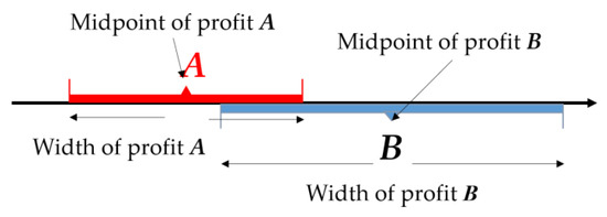
Figure 1.
Overlapping condition when comparing two intervals [17].
The pessimism degree-based method is implemented to conduct the tradeoff between the width and midpoint. The pessimism degree is a parameter within the range of [0,1] to define the willingness of a decision maker towards uncertainty. Higher pessimism indicates higher acceptance of uncertainty. The necessary and sufficient condition of is (9). Hence, by transforming the object function to the tradeoff function in (9), the width and midpoint of profit interval are comprehensively optimized. The mathematical proving process is based on fuzzy methodology. A more detailed introduction can be found in our previous work [17,32]. Research [30] first introduced this method in a study of coordinated dispatching of wind power and hydro power. Research [17] investigated the price taker VPP’s medium-term bidding strategy, representing UR and market price in interval numbers.
2.2. Market Structure and Price Maker Decition Procedure
In this paper, a typical pool-based two-stage market is applied. The market structure and VPP’s role are described in Figure 2.
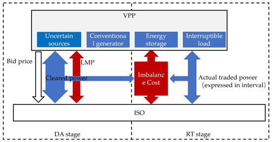
Figure 2.
Market and VPP operating process.
In the DA stage, VPP, power producers and demands submit hourly bid curves and capacity parameters to ISO for the next operating day. The bidding curve of the power producer is a non-decreasing piece-wise price function against power. On the other hand, the bidding curve of demand is a decreasing function [18,33].
Different from conventional producers or demands, VPP can aggregate DERs in a subsystem which exchanges power with the main grid through a common point. The EMS of VPP acts as a market agent and operator of those DERs. The VPP bid curve in this work is simplified as an hourly price like reference [21]. The simplification is effective because the producer bid curve slope is shallow. Moreover, it brings clearness in analysis. Similarly, many supply function researchers also use intercept as a bid strategy [33].
Notice that VPP is assumed to be the only strategic player in market, because this work is in the viewpoint of VPP. If the other market participants are assumed as strategic players, this work turns to market equilibria study; also, the related approach is different. The assumption here is the same as [2,20,21]. Therefore, the other producers and demands are bidding at their marginal cost or utility, which are therefore known to VPP [2,20].
In Figure 2, the white arrow is VPP’s bid price. The cleared power for each participant is figured out by ISO according to the bid curves. The blue arrows represent the power exchanges. LMP is calculated from the dual variable of the node power balance equation, which is also known as the shade price [34]. The DC load flow method is applied in network formulation. ISO pays for the cleared power of each participant at LMP. The red arrow is payment or purchase.
The RT market is operated minutes before actual power delivery [34]. In the RT market, participants who cannot meet up with the DA cleared power are charged. The shortage part according to the DA schedule is charged at Negative Deviation Price (NDP). NDP is higher than DA market LMP to ensure that VPP can buy the needed power to fill the gap. Meanwhile, surplus output is sold at the Positive Deviation Price (PDP). The PDP is relatively lower than the DA market LMP to ensure other market participants will buy the surplus part [1,19].
The decision makers of VPP predict the intervals of UR output. VPP also has to comprehensively consider the given NDP and PDP, the dispachable DER operation cost, the interruptible load cost, and retail price of the inner load. Provided with the above information, a VPP decision maker then optimizes the unbalanced cost, incomes and DA incomes and figures out the optimum bidding and scheduling strategy.
3. VPP Bidding and Scheduling Model
3.1. Upper Level Problem: VPP Strategy
The upper level problem aims at maximizing VPP’s profit. Due to uncertain resources in VPP, the expected profit is uncertain and is interpreted as an interval number. According to the Pessimism Degree (PD)-based interval ordering rule, the optimized results are calculated from the midpoint and width of profit referring to (10). PD indicates EMS’s preference between the expected profit value and uncertainty level .
where
In Equation (13), defines the income or payment to the main grid. is the LMP of node n where the VPP is connected. is the cleared power. It is positive when the VPPs supply redundant energy to DA market, and negative when VPPs purchase energy. Notice that both of them are decision variables of ISO in the lower level. is the income interval from the integrated load in VPP, and Equations (14) and (15) define the lowest and highest value. The consumed power interval in VPP reaches the bottom when the forecast load is at the left bound and IL is at the right bound and vice versa. The rest of the terms in (10)–(13) are hourly operation costs of CG, ES, deployed IL remedy and imbalance cost, respectively. is calculated as a portion of retail price . Equations (16) and (17) describe the imbalance cost interval bounds. The actual traded power interval with the main grid deviates from the DA cleared power. The negative deviation power is charged at , and the positive deviation power price is .
Constraint (18) represents the DA internal power balance of VPP. The left side of the equation is the schedule of VPP inner resources. The right side is scheduled power exchange. For clearness and efficiency, all the URs in VPP, which are uncontrollable, are accumulated to net output (19). are the midpoint of the forecast interval of UR representing the reference for the DA plan. The outputs of CG , ES devices , IL are strategically scheduled by EMS.
where
Constraints (20)–(24) show the RT inner power balance of VPP. Equation (20) defines the VPP scheduling mechanism during a power shortage occasion, while Equation (21) defines the power surplus occasion. Under the circumstance of net output shortage, EMS should activate the CG, discharge the ES devices and deploy IL at their maximum , , . Note that, the discharge power and IL are defined as positive. The opposite case mechanism is illustrated by (21).
where
Let both sides of Equation (21) be subtracted by Equation (20). The uncertainty mitigation strategy implemented by a controllable resource against UR is expressed in Equation (24). The net uncertainty of UR is supposed to be covered by the width of CG, ES, IL. Hence, the imbalance cost can be mitigated by those controllable resources, according to the definition of the imbalance cost (16) and (17).
Constraint (25) limits the strategic bidding price non-negative and no more than the market upper bound.
The following constraints illustrate the limits of individual components in VPP. Firstly, the reference value of uncertain power such as wind power should be inside the respective forecast interval (26) and (27).
Constraint (28) indicates the planned output of CG should be within the RT interval . Additionally, the top output in the balancing stage should not exceed its capacity .
Constraints (30) and (31) define that the discharge and charge power are non-negative and should be limited by ES maximum power . Equation (32) calculates the power output of ES. It is negative when ES is charging. Similar to other VPP components, the ES DA planned output should be in the interval of the RT stage (33). In constraint (34), the residue capacity should be within the device capacity at any time. Constraints from (35) to (39) illustrate the RT stage limits of ES. Equations (35) and (36) define the left and right bounds of ES power output based on the combination of the bounds of charging and discharging behavior. In (38), ES is in the case of the most fully charged or lowest discharged. Hence, its residue capacity should be no more than the device upper limit. On the contrary, the mechanism is mirrored in (39).
Constraint (40) sets the bounds of the DA planned value of IL. The deployed IL is constrained to a portion of the lowest predicted load outcome . is a given factor.
3.2. Lower Level Problem: ISO Market Clearing Simulation
The lower lever problem aims at maximizing social utility in the view of ISO operating the main grid. The three product terms in (41) are from demands, VPP and other generating companies in sequence. Note that the VPP bid price is strategically decided, while others are non-strategic and stick to their marginal cost, and , respectively. The bidding price is a decision variable of the upper level and input as parameter in the lower level problem.
The following are the constraints of the lower lever problem. Equation (42) manifests the main grid DA market power balance. For any node and time slot, the net generated and consumed power is equal to the total injection power. is the node where the VPP managed sub system is connected. represents transmission lines connecting node n. All the variables on the right side of the colon are dual variables in the following context. Here, LMP is the shade price. It economically interprets the scarcity of certain resources which represent the available electricity here. The shade price is widely utilized as DA market LMP in many studies.
Constraint (43) is the upper and lower limits of cleared power submitted by VPP to ISO, deduced from (44) and (45), i.e., the upper bound is the top level of UR, ES discharge rate, CG and IL (44). The limits are time varying due to the uncertain resources. The corresponding dual variables of up and down inequalities are and , respectively.
where
Constraints (46) and (47) illustrate the limits of cleared power submitted by non-strategic producer and demands.
Constraint (48) defines the power flow limits of transmission line. The load angle of each node constraint is shown in (49), and node1 is set to be the reference bus and the load angle is 0 at any time (50).
3.3. Model Transformation and Linearization
The lower level problem is linear and convex. Therefore, its optimality can be substituted by Karush-Kuhn-Tucker (KKT) optimality conditions, which are listed in Appendix A. However, the product in the upper level problem is not linear because both and are decision variables. Referring to [18,21], the linearization process utilizes the strong duality condition and complementary slackness condition with the KKT equation to derive the linearized form (51). The detail process is listed in Appendix B.
All the complementary slackness conditions are nonlinear because of the product of dual variable and primal variable. This linearization is realized by introducing an additional binary decision variable . is given a large enough constant, which is around 100 times that of the corresponding dual variable. The linearized form of (43) is (52)–(55), while the rest is described in Appendix B.
4. Case Studies
4.1. Parameters
The main grid system topology in Figure 3 is modified based on a network provided by reference [18]. The left side of the network is formed as a source side, while the right side of the network is the demand side. The generating companies O1, O2, O3 operate large conventional generators referring to rows 1 to 3 of Table 1. The major demands D2, D3, D4 are located on the right side. The total demand is 800 MW. D1, D2, D3 and D4 share 10%, 30%, 30% and 30% of the total demand, respectively. D1 represents those industrial loads directly supplied by generators in practice. Hence, line 2–4 and line 3–6 basically transmit power from the source side on the left to the demand side on the right. The susceptance of all the transmission line of the main grid is 9.412 per unit [18].
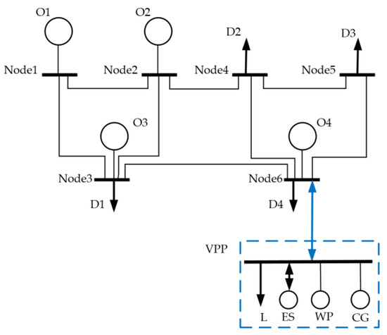
Figure 3.
System topology and VPP structure.

Table 1.
Parameters of competitive market players [18].
Both generating companies and load bidding curve parameters are from [18]. The generating companies O1, O2, O3, O4 bid competitively at marginal cost. Table 1 offers bidding curve parameters. The capacity of each power block is from row 4 to 7 in Table 1. The respective cost or bidding price is from row 8 to 11 in Table 1. Therefore, a piece-wise bidding curve for each generating company is formed.
Figure 4 depicts the time varying curves of D4 intuitively. All four demands share the same bid curve, and also bid competitively at marginal utility. The blocks of each demand share 90%, 2.5%, 2.5%, 2.5%, 2.5% of their maximum in sequence. For example, the maximum demand of D4 is 240 MW, which is obtained from the total demand 800 MW multiplied by the percentage 30%. The maximum power of each respective demand block is <216, 6, 6, 6, 6> MW. The bid price in the order of blocks is <24.968, 22.628, 20.876, 20.606, 20.378>$/MWh in hour 11. The demand bid curve is generally high in peak hours and low in valley hours. Detailed parameters of the four demands refer to Table 2 in [18].
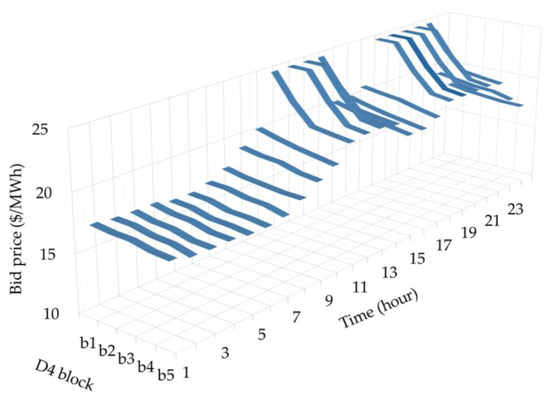
Figure 4.
Hourly bid curve of demand D4.
Node 6, which is on the demand side, is modified. A subsystem containing Wind Power (WP), Conventional Generator (CG), Energy Storage (ES) devices and Interruptible Load (IL) is connected. VPP manages these demand side distributed resources and acts as a single participant in the market. Among the aggregated resources, the marginal cost of CG is 20.3$/MW and the capacity is 40 MW. Parameter ES is from reference [35]. It has a maximum level of 30 MWh and the initial status is 8 MWh. Both the charge and discharge maximum power are 4.5 MW with the efficiency factor at 0.9. The operation cost is 9.2$/MW. The installed capacity of WP is 125 MW and the wind speed parameter is from Bishop Clerks data [36]. WP is calculated from wind speed according to the method in reference [37]. The load data are from the PJM historical data miner [38]. The calculated net output of UR of VPP according to (20)–(24) is depicted in Figure 5. The red intervals on the top of the bars describe the width of the hourly forecast value, while the height of the blue bars is the midpoint. The width in practice can be wide enough to cover all possible value. Here, in case 1, the width is set 5% of the mid value. The negative parts in Figure 5 show that the load is higher than renewable power in these time slots. The network constraints of the subsystem are not considered due to the relatively small scale.
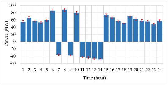
Figure 5.
Forecast net output interval of UR in VPP.
Apart from VPP, generating company O4 is also connected with node 6 to analyze the interaction with VPP. Its capacity is relatively small, representing non-strategic distributed generation.
The retail price is typical peak, valley, shoulder price. The IL remedy is set to be 0.7 times of the retail price. PDP and NDP are set to 0.4 and 1.8 times, respectively, of DA market price. All the hourly price curves are shown in Figure 6.
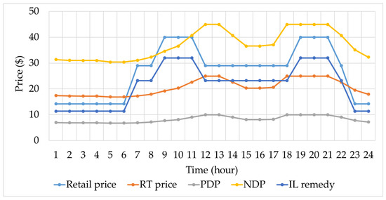
Figure 6.
Price parameters.
Finally, the model is solved by IBM ILOG CPLEX Optimization Studio 12.4, which is widely used in solving MILP.
4.2. VPP Bid and Scheduling Results in DA Market
In case 1, we investigate the optimized VPP strategy in the DA market based on the parameter setting in the second column of Table 2. All the parameter settings of the other following cases are also consolidated in this table.
Table 2.
Parameter setting of cases.
The optimized bid price of VPP directly affects DA market clearing and it equals the DA LMP of node 6. As the blue line with dots in Figure 7 shows, the peak LMP of 24.968$/MWh occurs in hour 12, 13 and hour 18–21, while the lowest LMP is 16.886$/MWh in hour 5 and 6. Figure 7 also shows the power flow of node 6 where VPP is located. The positive bars in stack column diagram represent power injected into node 6, while the negative bars represent power consumed. For example, the black bars represent the cleared competitive demand D4, while purple bars represent the cleared power of VPP.
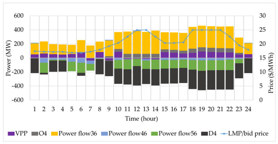
Figure 7.
LMP of node 6 and cleared power.
In hour 5, VPP bids at 16.886$/MWh, equal to the LMP. The bid price of the first block of D4 is also 16.886$/MWh, as Figure 4 shows. Therefore, the cleared power should be within the first block of D4, due to the decreasing demand bidding curve. In this case, the cleared demand of D4 is 0s, because the valley demands bid is low. Therefore, the strategic VPP bidding price made the traded power to D4 zero. On the other hand, the cleared power of VPP is 56.631 MW. The power flow of line 3–5, line 4–5, line 5–6 is 131.874 MW, −53.670 MW and −134.835 MW, respectively. Based on power flows of related lines, the UR output is scheduled to supply other nodes. The resulting DA income of this hour is 956.271$. To conclude, VPP manipulates the LMP to decide the cleared power. If the offering price of demand is low, its strategy will limit the cleared power.
In hour 18, the peak demand status occurs as Figure 4 shows. VPP bids at 24.968$/MW. The bid curve of D4 is <25, 24.968, 22.628, 20.876, 20.606>$/MW in the order of blocks. Hence, the LMP is 24.968$/MW at the second block. The cleared power of D4 is 216 MW, which is much higher than the outcome of hour 5. Therefore, VPP’s bid let more demand to be cleared considering the profitable peak hour price. The traded power is 73.84 MW. It is also higher than the cleared power of hour 5. The resulting DA income of this hour increases to 1843.637$. Besides, considering the high market price, O4 is also fully activated at 60 MW as the grey bar shows. Therefore, VPP strategically bids for more scheduled power and thus more income when demand bids are high.
In hour 24, VPP bids and manipulates LMP to 17.94$/MWh, which is lower than all the bid prices of O4 referring to column 5 of Table 1. Consequently, O4 is not activated. In contrast, the cleared power for VPP is 54.719 MW. Furthermore, the predicted UR output in VPP of this moment is [49.96, 65.76] MW. This means VPP utilizes the zero cost UR to bid at a low price. Contrarily, O4 is a competitive conventional generator and its bid price is fixed and relatively high. To conclude, VPP can strategically manipulate the LMP to let its resources scheduled in prior to the other competitive generator on the same node.
Figure 8 offers a further detailed allocation of VPP inner controllable resources and traded power in DA stage. The blue bars show that from hour 1 to 6,8,10 and 15 to 24, the UR net output is abundant. As the red bars show, the traded power is slightly lower than the UR net output. Therefore, most of the UR output is sold to the main grid.
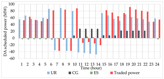
Figure 8.
DA scheduled power of VPP components.
From hour 24 to 6, demand is at a valley status. ES charges in these hours, as the green bars show. For example, ES charges at 3.533 MW in hour 2 and discharges at 4.5 MW in hour 12. Referring to the LMP curve, LMP is at the lowest level during that period. For instance, LMP is 17.25$/MWh in hour 6 and 24.968$/MWh in hour 12. The LMP is relatively not profitable in valley hours. It can be deduced that ES charges in valley hours for use in peak hours.
From hour 11 to 14, net output of UR is negative, and CG is activated to fill the shortage as the black bars depict. VPP turns to purchase energy from the market as the red bars show. Especially in hour 12, the schedule UR is −43.56 MW. CG’s output reaches its maximum 40 MW. ES then discharges. CG is applied in priority to cover the inner shortage because of the lower cost compared to ES.
From hour 15 to hour 22, the LMP is higher than the generation cost 20.3$/MW. For example, the LMP of hour 18 is 24.968$/MW. The traded power, the schedule UR and CG are 73.84 MW, 51.31 MW, 22.53 MW, respectively. CG and UR output comprise the scheduled power. Therefore, CG is activated to supply the DA market for profit.
To conclude, the controllable inner resources are coordinately optimized. ES is utilized to shift power from valley hours to peak hours, and CG and ES are operated to fill the power shortage and profit in peak hours.
Based on the setting of case 1, we impose a network-congested condition. The calculated power flow of line 2–4 and line 3–6 is 290.911 and 252.293 MW, respectively, in hour 17. Then, we limit the transmission line capacity to be slightly lower than the calculated value, as the third column of Table 3 shows. Results show the bid price of VPP increases from 20.606$/MW to 20.876$/MW. The LMP of node 6 is higher than any of other nodes. For instance, the LMP of node 3 is 20.606$/MW. Meanwhile, the cleared power is not changed according to the fourth row. Consequently, VPP gets more income from the DA market according to the fifth row. It can be deduced that VPP can utilize the network congestion and gain more profit by strategically increasing LMP.
Table 3.
The strategy of VPP when the network is congested.
4.3. VPP Uncertainty Mitigation Results in the RT Market
Switching to the RT stage, we analyze the interval optimization-based imbalance mitigation mechanism coping with uncertainty. According to (20)–(24), the input uncertainty is caused by UR, and should be mitigated by controllable resources to restrain the deviation of traded power. Figure 9 compares the uncertainty inputted by UR with the mitigated uncertainty of traded power. The interval width remarkably shrinks in peak hours, e.g. in hour 19, the NDP and PDP are 44.9424 $/MWh and 9.9872 $/MWh, respectively. The UR is [61.90,78.82] MW while traded power is [91.9, 91.9] MW, which means the uncertainty turns to zero. Hence, the proposed uncertainty mitigation method is effective in peak hours. It can even wipe out the entire uncertainty.
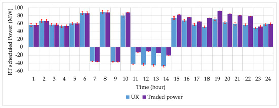
Figure 9.
The hourly interval width of UR and traded power.
In those valley hours, the interval width decease only a little. For example, in hour 8, the NDP and PDP are 32.292$/MWh and 7.176$/MWh, respectively. The UR is [53.23, 66.37] MW while traded power is [84.18, 92.21] MW. The width declines from 4.434 to 4.015 because the NDP and PDP are amplified or reduced from the DA reference price, respectively. The NDP and PDP of valley hours are relatively not as severe as the price of hour 8 shows. Consequently, the uncertainty mitigation is not evident during those periods.
Figure 10 further dissects the contributions of CG, ES, IL in mitigating the uncertainty of actual traded power. The length of the stacked bars represents the contribution of each controllable resource, and the summed value in each time slot equals the UR interval width. During peak hours, such as from hour 15 to 22, CG is utilized to cover all the widths. From hour 24 to 7, IL and ES are deployed instead of CG. For instance, ES and IL offer uncertainty mitigation of 1.502 MW and 1.996 MW, respectively, in hour 1.
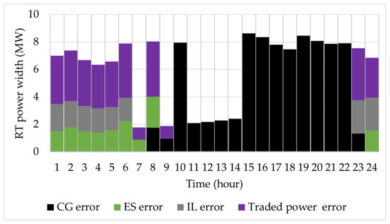
Figure 10.
Deployed controllable resource power widths.
The contributions of DERs change among different hours because of their time varying deployment cost. For example, the IL remedy is 11.376$/MWh in hour 1 and 32$/MWh in hour 19. Hence, VPP tends to curtail load in valley hours. Similarly, the PDP and NDP are 6.972$/MWh 31.374$/MWh in hour 1, 9.9872$/MWh and 44.9424$/MWh in hour 19. During valley periods, VPP can afford a part of deviation cost as the charge is relatively low. To summarize, the uncertainty mitigation mechanism can decrease the uncertainty by coordinately deploying various controllable resources considering the deployment cost.
In order to value the contribution of controllable resources, none of the controllable resources is involved in case 2 to make the comparison. The calculated imbalance cost interval is [−1311.64, 437.21]$. In contrast, with the aid of CG and IL, the imbalance cost interval of case 1 is [0, 486.99]$. Therefore, the interval optimization-based imbalance cost mitigation mechanism can effectively decrease the uncertainty and hence restrain the imbalance cost.
4.4. Sensitivity analysis
Given different levels of NDP and PDP in case 3, the optimized profit and imbalance cost are calculated in Table 4. With the increase of NDP and decrease of PDP factor in the first column, the NDP increases and PDP decreases. The left bound of the imbalance cost in the second column shows that penalty paid for traded power of negative deviation decreases as the NDP increases. Note that the left bound in the first row is −632.14$. The negative value denotes that VPP has to pay 632.12$ to the market operator. From the second row, EMS strictly manages the negative deviation; hence, no penalty occurs with the increasing NDP. On the other hand, the right bound of the imbalance cost shows that income from traded power of positive deviation reduces as the PDP increases, because it is becoming less profitable.
Table 4.
Profit and Imbalance cost against different levels of NDP & PDP.
The third column shows the total profit interval of VPP. As NDP increases with decreasing PDP, the profit width increases from 1129.5$ to 1760.5$ according to the fourth column. Simultaneously, the profit midpoint increases from 16,754.5$ to 17,396.5$ according to the fourth column. This indicates that higher level negative deviation charges and lower profitable positive deviation price will allow VPP to achieve higher expected profit with more uncertainty.
In case 4, the width-midpoint ratio of UR is adjusted from 5% to 15% to find the effect of predefined UR uncertainty on the outcome of profit. As column 2 of Table 5 shows, the right bound of the imbalance cost interval increases with the width-midpoint ratio of UR. Consequently, both the left and right bounds of optimized VPP total profit in column 3 are decreased. According to column 4, the increasing predefined uncertainty simultaneously increases the uncertainty of optimized profit and decreases the expected profit denoted by column 5. Therefore, the price maker of VPP should carefully set the interval width of uncertain variables. Although decision makers can use wider intervals to cover more possibility in forecasts, the optimized result will also be more uncertain.
Table 5.
Profit and Imbalance cost of different UR width-midpoint ratios.
In case 5, the relationship between PD and optimized profit is investigated. The right bound and midpoint of total profit increase with PD as the top of the red interval and blue bars show in Figure 11. When PD is 0.1, the profit interval is [15,841, 18,572]$. When PD is beyond 0.6, the profit interval becomes stable at [15,283, 21,156]$. The minimum width of profit is 1365.5 when PD is 0.1. The width holds at 2936.5 from PD 0.6 to PD 0.9. Both the profit interval and midpoint increase with the pessimism degree of VPP decision makers. Therefore, if a decision maker of VPP assumes higher PD, higher possible profit with more uncertainty will be pursued.
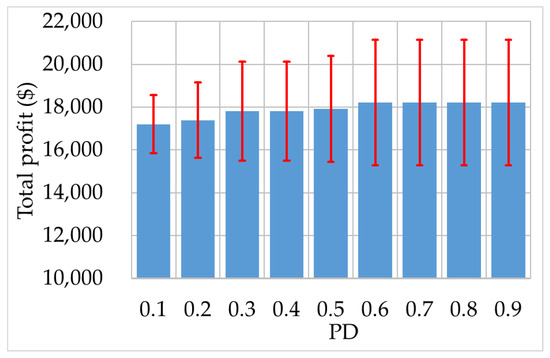
Figure 11.
The optimized profit interval against PD.
5. Conclusions
Among the existing works, this study argues that VPP is a price maker stead of a price taker. Compared with other price maker research, various DERs are integrated to operate coordinately in the manner of VPP. Moreover, the interval optimization method is utilized instead of stochastic optimization. The proposed two-stage bi-level bidding and scheduling interval optimization model is applied to optimize VPP’s strategy in the DA and RT market. In the DA stage, optimized results show that VPP’s bidding price manipulates the LMP to limit the scheduled power in valley hours and increase its income in peak hours. Compared with a competitive conventional generator on the same node, VPP bids strategically and lets its resources scheduled in prior to the other competitive generator on the same node by utilizing zero-cost UR. VPP can also optimally schedule the ES to shift power from valley hours to peak hours. Inner CG is flexibly applied to cover the inner power shortage and to profit from the market during peak hours. In a network-congested case, VPP will strategically bid higher for more profit. In the RT stage, the proposed interval optimization-based mechanism can effectively reduce the deviation of traded power from the DA schedule and hence restrain the imbalance cost. Various controllable resources are coordinately applied to reduce the uncertainty. A negative imbalance cost can even be entirely wiped out if the NDP is high. Finally, sensitivity analysis shows that VPP tends to achieve higher expected profit with higher uncertainty when NDP is high and PDP is low. The input width of uncertain variables should be carefully set. A wider interval width setting by VPP will increase the uncertainty of results and decrease the expect profit. Last but not least, VPP decision makers of high PD tend to achieve high profit and uncertainty. Since this work is in the viewpoint of strategic VPP, our future work will study the interaction among multi strategic market participants.
Author Contributions
Methodology, formal analysis, investigation, writing J.H.; writing—review and editing, C.J. and Y.L.
Funding
This work was supported in part by the National Natural Science Foundation of China (No. 51907092).
Conflicts of Interest
The authors declare no conflict of interest.
Nomenclature
| Sets: | or | Forecast WP interval (MW) | |
| Market participants connecting to node | or | Forecast load interval (MW) | |
| transmission lines connecting to node | Maximum bid price in DA market ($/MW) | ||
| Indexes: | Maximum power of ES (MW) | ||
| The left and right bounds of interval | , | Initial, minimum and maximum capacity of ES (MWh) | |
| Index for Time slots | , | Charging and discharging efficiency factor | |
| Index for competitive producer | Available interruptible load factor | ||
| Index for generation blocks of competitive producer | Susceptance of line (per unit) | ||
| Index for blocks of demand | Capacity of line (MW) | ||
| Parameters or constants: | Variables: | ||
| VPP Bid price in time slot t ($/MW) (MW) | Cleared power of VPP in time slot (MW) | ||
| Cleared power of block of demand in time slot (MW) | Scheduled power of CG in DA stage in time slot (MW) | ||
| Cleared power of block of producer in time slot (MW) | Scheduled power of ES in DA stage in time slot (MW) | ||
| Retail market price ($/MW) | Deployed IL in DA stage in time slot (MW) | ||
| Marginal utility of block of demand in time slot ($/MW) | or | Interval of VPP traded power in RT stage in time slot (MW) | |
| Marginal cost of block of producer in time slot ($/MW) | or | Interval of CG output in RT stage in time slot (MW) | |
| Upper limit of block of producer (MW) | or | Interval of ES output in RT stage in time slot (MW) | |
| Upper limit of block of demand in time slot (MW) | or | Interval of ES discharging in RT stage in time slot (MW) | |
| Reference of forecast WP interval (MW) | or | Interval of ES charging in RT stage in time slot (MW) | |
| Reference of forecast load interval (MW) | or | Interval of deployed IL in RT stage in time slot (MW) | |
| Load angle of node in time slot (rad) | |||
Appendix A
First order optimality conditions:
The complementary slackness conditions:
Appendix B
1. Linearization of the complementary slackness conditions:
Step 1: build the relationship between and
According to the KKT condition (A1),
Deduced from complementary slackness condition (A7):
Deduced from complementary slackness condition (A6):
Thus:
Step 2: linearization of by strong duality condition
The strong duality condition of the lower level problem stands because of convexity. Therefore, the maximization of lower level problem equals the minimization of its dual problem. in (41) can be expressed as:
Thus:
2. Linearization of the complementary slackness conditions (A6), (A7):
Linearization of (A8), (A9):
Linearization of (A10), (A11):
Linearization of (A12), (A13):
Linearization of (A14), (A15):
References
- Pandzic, H.; Morales, J.M.; Conejo, A.J.; Kuzle, I. Offering model for a virtual power plant based on stochastic programming. Appl. Energy 2013, 105, 282–292. [Google Scholar] [CrossRef]
- Baringo, L.; Conejo, A.J. Strategic Offering for a Wind Power Producer. IEEE Trans. Power Syst. 2013, 28, 4645–4654. [Google Scholar] [CrossRef]
- Pudjianto, D.; Ramsay, C.; Strbac, G. Virtual power plant and system integration of distributed energy resources. IET Renew. Power Gener. 2007, 1, 10–16. [Google Scholar] [CrossRef]
- Nosratabadi, S.M.; Hooshmand, R.-A.; Gholipour, E. A comprehensive review on microgrid and virtual power plant concepts employed for distributed energy resources scheduling in power systems. Renew. Sustain. Energy Rev. 2017, 67, 341–363. [Google Scholar] [CrossRef]
- Gawel, E.; Purkus, A. Promoting the market and system integration of renewable energies through premium schemes—A case study of the German market premium. Energy Policy 2013, 61, 599–609. [Google Scholar] [CrossRef]
- Rahimiyan, M.; Baringo, L. Strategic Bidding for a Virtual Power Plant in the Day-Ahead and Real-Time Markets: A Price-Taker Robust Optimization Approach. IEEE Trans. Power Syst. 2016, 31, 1–12. [Google Scholar] [CrossRef]
- Asmus, P. Microgrids, Virtual Power Plants and Our Distributed Energy Future. Electr. J. 2010, 23, 72–82. [Google Scholar] [CrossRef]
- Pasetti, M.; Rinaldi, S.; Manerba, D. A Virtual Power Plant Architecture for the Demand-Side Management of Smart Prosumers. Appl. Sci. 2018, 8, 432. [Google Scholar] [CrossRef]
- Howell, S.; Rezgui, Y.; Hippolyte, J.-L.; Jayan, B.; Li, H. Towards the next generation of smart grids: Semantic and holonic multi-agent management of distributed energy resources. Renew. Sustain. Energy Rev. 2017, 77, 193–214. [Google Scholar] [CrossRef]
- Li, S.; Park, C.S. Wind power bidding strategy in the short-term electricity market. Energy Econ. 2018, 75, 336–344. [Google Scholar] [CrossRef]
- Hong, Y.-Y.; Weng, M.-T. Optimal short-term real power scheduling in a deregulated competitive market. Electr. Power Syst. Res. 2000, 54, 181–188. [Google Scholar] [CrossRef]
- Tajeddini, M.A.; Rahimi-Kian, A.; Soroudi, A. Risk averse optimal operation of a virtual power plant using two stage stochastic programming. Energy 2014, 73, 958–967. [Google Scholar] [CrossRef]
- Peik-herfeh, M.; Seifi, H.; Sheikh-El-Eslami, M.K. Two-stage approach for optimal dispatch of distributed energy resources in distribution networks considering virtual power plant concept. Int. Trans. Electr. Energy Syst. 2014, 24, 43–63. [Google Scholar] [CrossRef]
- Shayegan-Rad, A.; Badri, A.; Zangeneh, A. Day-ahead scheduling of virtual power plant in joint energy and regulation reserve markets under uncertainties. Energy 2017, 121, 114–125. [Google Scholar] [CrossRef]
- Peik-Herfeh, M.; Seifi, H.; Sheikh-El-Eslami, M.K. Decision making of a virtual power plant under uncertainties for bidding in a day-ahead market using point estimate method. Int. J. Electr. Power Energy Syst. 2013, 44, 88–98. [Google Scholar] [CrossRef]
- Fan, S.; Piao, L.; Ai, Q. Fuzzy day-ahead scheduling of virtual power plant with optimal confidence level. IET Gener. Transm. Distrib. 2016, 10, 205–212. [Google Scholar] [CrossRef]
- Hu, J.; Liu, Y.; Jiang, C. An optimum bidding strategy of CVPP by interval optimization. IEEJ Trans. Electr. Electron. Eng. 2018, 13, 1568–1577. [Google Scholar] [CrossRef]
- Ruiz, C.; Conejo, A. Pool Strategy of a Producer With Endogenous Formation of Locational Marginal Prices. IEEE Trans. Power Syst. 2009, 24, 1855–1866. [Google Scholar] [CrossRef]
- Sharma, K.C.; Bhakar, R.; Tiwari, H. Strategic bidding for wind power producers in electricity markets. Energy Convers. Manag. 2014, 86, 259–267. [Google Scholar] [CrossRef]
- Kazempour, S.J.; Conejo, A.J.; Ruiz, C. Strategic Bidding for a Large Consumer. IEEE Trans. Power Syst. 2015, 30, 848–856. [Google Scholar] [CrossRef]
- Daraeepour, A.; Kazempour, J.; Patiño-Echeverri, D.; Conejo, A.J. Strategic Demand-Side Response to Wind Power Integration. IEEE Trans. Power Syst. 2016, 31, 3495–3505. [Google Scholar] [CrossRef]
- Cui, H.; Li, F.; Hu, Q.; Bai, L.; Fang, X. Day-ahead coordinated operation of utility-scale electricity and natural gas networks considering demand response based virtual power plants. Appl. Energy 2016, 176, 183–195. [Google Scholar] [CrossRef]
- Shafiekhani, M.; Badri, A.; Shafie-khah, M.; Catalão, J.P.S. Strategic bidding of virtual power plant in energy markets: A bi-level multi-objective approach. Int. J. Electr. Power Energy Syst. 2019, 113, 208–219. [Google Scholar] [CrossRef]
- Riveros, J.Z.; Bruninx, K.; Poncelet, K.; D’Haeseleer, W. Bidding strategies for virtual power plants considering CHPs and intermittent renewables. Energy Convers. Manag. 2015, 103, 408–418. [Google Scholar] [CrossRef]
- Karimyan, P.; Hosseinian, S.H.; Khatami, R.; Abedi, M. Stochastic approach to represent distributed energy resources in the form of a virtual power plant in energy and reserve markets. IET Gener. Transm. Distrib. 2016, 10, 1792–1804. [Google Scholar] [CrossRef]
- Zamani, A.G.; Zakariazadeh, A.; Jadid, S.; Kazemi, A. Stochastic operational scheduling of distributed energy resources in a large scale virtual power plant. Int. J. Electr. Power Energy Syst. 2016, 82, 608–620. [Google Scholar] [CrossRef]
- Ju, L.; Li, H.; Zhao, J.; Chen, K.; Tan, Q.; Tan, Z. Multi-objective stochastic scheduling optimization model for connecting a virtual power plant to wind-photovoltaic-electric vehicles considering uncertainties and demand response. Energy Convers. Manag. 2016, 128, 160–177. [Google Scholar] [CrossRef]
- Saric, A.; Stankovic, A. An Application of Interval Analysis and Optimization to Electric Energy Markets. IEEE Trans. Power Syst. 2006, 21, 515–523. [Google Scholar] [CrossRef]
- Wu, L.; Shahidehpour, M.; Li, Z. Comparison of Scenario-Based and Interval Optimization Approaches to Stochastic SCUC. IEEE Trans. Power Syst. 2012, 27, 913–921. [Google Scholar] [CrossRef]
- Liu, Y.; Jiang, C.; Shen, J.; Hu, J. Coordination of Hydro Units With Wind Power Generation Using Interval Optimization. IEEE Trans. Sustain. Energy 2017, 6, 443–453. [Google Scholar] [CrossRef]
- Sengupta, A.; Pal, T.K. On comparing interval numbers. Eur. J. Oper. Res. 2000, 127, 28–43. [Google Scholar] [CrossRef]
- Sengupta, A.; Pal, T.K. On Comparing Interval Numbers: A Study on Existing Ideas; Springer: Berlin/Heidelberg, Germany, 2009. [Google Scholar]
- Hobbs, B.; Metzler, C.; Pang, J.-S. Strategic gaming analysis for electric power systems: An MPEC approach. IEEE Trans. Power Syst. 2000, 15, 638–645. [Google Scholar] [CrossRef]
- Dai, T.; Qiao, W. Finding Equilibria in the Pool-Based Electricity Market with Strategic Wind Power Producers and Network Constraints. IEEE Trans. Power Syst. 2016, 32, 389–399. [Google Scholar] [CrossRef]
- Alharbi, H.; Bhattacharya, K. Stochastic Optimal Planning of Battery Energy Storage Systems for Isolated Microgrids. IEEE Trans. Sustain. Energy 2018, 9, 211–227. [Google Scholar] [CrossRef]
- University of Massachusetts Amherst, Wind Energy Center. Available online: https://www.umass.edu/windenergy/resourcedata (accessed on 1 July 2019).
- Karki, R.; Hu, P.; Billinton, R. A Simplified Wind Power Generation Model for Reliability Evaluation. IEEE Trans. Energy Convers. 2006, 21, 533–540. [Google Scholar] [CrossRef]
- PJM Data Directory. 2019. Available online: https://www.pjm.com/markets-and-operations/data-dictionary.aspx (accessed on 1 July 2019).
© 2019 by the authors. Licensee MDPI, Basel, Switzerland. This article is an open access article distributed under the terms and conditions of the Creative Commons Attribution (CC BY) license (http://creativecommons.org/licenses/by/4.0/).