Article

A Mixed-Integer Convex Programming Algorithm for Security-Constrained Unit Commitment of Power System with 110-kV Network and Pumped-Storage Hydro Units

1
School of Electric Power Engineering, South China University of Technology, Guangzhou 510640, China
2
The Power Dispatching Control Center of Shenzhen Power Supply Bureau, Shenzhen 518001, China
3
Department of Electrical and Computer Engineering, University of Central Florida, Orlando, FL 32816, USA
*
Author to whom correspondence should be addressed.
Energies 2019, 12(19), 3646; https://doi.org/10.3390/en12193646
Submission received: 22 August 2019 / Revised: 22 September 2019 / Accepted: 23 September 2019 / Published: 24 September 2019

Abstract

:
The secure operation of 110-kV networks should be considered in the optimal generation dispatch of regional power grids in large central cities. However, since 110-kV lines do not satisfy the premise of R << X in the direct current power flow (DCPF) model, the DCPF, which is mostly applied in the security-constrained unit commitment (SCUC) problem of high-voltage power grids, is no longer suitable for describing the active power flow of regional power grids in large central cities. Hence, the quadratic active power flow (QAPF) model considering the resistance of lines is proposed to describe the network security constraints, and an SCUC model for power system with 110-kV network and pumped-storage hydro (PSH) units is established. The analytical expressions of the spinning reserve (SR) capacity of PSH units are given considering different operational modes, and the SR capacity of PSH units is included in the constraint of the SR capacity requirement of the system. The QAPF is a set of quadratic equality constraints, making the SCUC model a mixed-integer nonlinear non-convex programming (MINNP) model. To reduce the computational complexity of solving the model when applied in actual large-scale regional networks, the QAPF model is relaxed by its convex hull, and the SCUC model is transformed into a mixed-integer convex programming (MICP) model, which can be solved to obtain the global optimal solution efficiently and reliably by the mature commercial solver GUROBI (24.3.3, GAMS Development Corporation, Guangzhou, China). Test results on the IEEE-9 bus system, the PEGASE 89 bus system and the Shenzhen city power grid including the 110-kV network demonstrate that the relaxed QAPF model has good calculation accuracy and efficiency, and it is suitable for solving the SCUC problem in large-scale regional networks.

Graphical Abstract

1. Introduction

SCUC is an optimization problem in power grids to determine the generator units’ on-off states and power output within a certain dispatch period while minimizing the total operation cost. The constraints include unit operation characteristics, transmission network security, and load demand. SCUC is fundamental to the day-ahead generation dispatch scheduling in power system operation. The modeling and solution methods of the SCUC problem have been deeply studied. The DCPF model is most commonly used to describe the network security constraints in the SCUC model [1,2,3,4,5]. In [1], the SCUC model considering the transmission capacity limit is solved by a Lagrangian relaxation method. Benders decomposition is also widely used: in [2], transmission switching constraints are introduced in subproblems for easing transmission violations, and in [3], committable and uncommittable unit states are introduced to reduce the number of integer variables in the master problem, thereby enhancing the efficiency of solving SCUC problems in large-scale power grids. Besides, when the frequency response is addressed, a piece-wise linearization technique is employed to handle the nonlinear function representing the minimum frequency [4]. In [5], generalized generation distribution factors are utilized to reformulate the SCUC problem into a linear form. However, the accuracy of the DCPF model for representing power flow is guaranteed only when the resistance is much smaller than the reactance of lines. Recently, with load demand increasing rapidly and the scale of grids expanding quickly, the regional grids in metropolises are becoming complicated. Since these grids are mainly composed of 110-kV networks, the secure operation of 110-kV networks should be considered when optimizing the generation dispatch scheduling of these regional grids. Since the reactance of lines is about four to five times the resistance in 110-kV networks, the resistance should not be omitted when representing the security constraints, making the SCUC problem based on the DCPF model no longer applicable in power grids including 110-kV networks.
To capture the active power of lines more accurately, the alternating current power flow (ACPF) model is applied. The SCUC problem with ACPF constraints is usually decomposed into a UC master problem and ACPF security-checking subproblems and solved alternately. Simplified approximation of the ACPF model is another solution method to decrease computational burden. With conic approximations, the SCUC model with ACPF constraints is transformed into a mixed-integer second-order cone programming (MISOCP) model to reduce the computational complexity [6]. Another approach for approximating the ACPF constraints is by Taylor series expansion and adapted step-size region, where the constraints that would never bind are excluded [7]. For a stochastic SCUC problem with wind power volatility, Lagrangian relaxation is applied for parallel computation, but the original nonlinear model is piece-wise linearized, and the iteration process is still burdensome [8]. To guarantee the global solution at convergence, in [9], optimization-based bounds tightening, second-order cone relaxations, and piece-wise outer approximations are leveraged. Though the ACPF model is more accurate, the constraints are non-convex and nonlinear, and therefore the computation burden and complexity are extremely high when applied to the large-scale grids. In [10], the ACPF model is decomposed into linear formulas with two separable parts corresponding to the voltage magnitudes and voltage angles, respectively. Though the decomposition is a decent approximation of the ACPF model when the networks is with lines of low X/R ratio, the reactive power of load nodes is needed at first. In addition, Benders decomposition is applied to deal with the SCUC problem with ACPF constraints considering wind power uncertainty, however, computational efficiency may decrease significantly as the scale of the network expands [11,12,13,14]. Since the reactive power of load nodes cannot be exactly forecast at present, the reactive power of load nodes is difficult to consider in the practical scheduling of day-ahead generation dispatch. Besides, the reactive power regulation and voltage control of the system are typically performed after the day-ahead generation dispatch schedule has been determined. Therefore, we only pay attention to the active power distribution in the optimal day-ahead generation dispatch problem. Consequently, it is more practical to simplify the ACPF model to reduce the computation burden while maintaining a more accurate formulation than the DCPF model to represent the relationship between branch active power and node injected active power.
PSH units are special forms of generators, which can smoothly accommodate the load fluctuation, and they are widely used in modern grids. For large-scale regional grids with vast capacity nuclear units and heavy loads, PSH units can contribute to stabilizing the power output of nuclear units. In addition, the output of PSH units can change swiftly to accommodate the uncertain power fluctuation, and the quick adjustment of the SR capacity can relieve the impact from uncertain load forecast and renewable output to the grid. Therefore, the contribution of PSH units should be considered in the scheduling of day-ahead generation dispatch in large-scale regional grids. Many studies have been conducted on the modeling of PSH units in SCUC and economic dispatch problems, but there is a lack of research on formulating the SR capacity of PSH units. In [15,16,17], the cooperation of wind power and PSH units was studied without considering the SR capacity from PSH units. In [18,19], the SR capacity was included in optimal generation dispatch, but the difference in SR capacity among different operation modes of PSH units was neglected. Therefore, how to represent the SR capacity supplied by PSH units in the SCUC or optimal dispatch model needs further research.
The major contributions of this study are twofold: (1) An SCUC model of a power system with 110-kV network and PSH units is established, in which the QAPF model that considers the impact of resistance of lines is proposed to formulate the network security constraints, and the novel formulation of SR capacity of PSH units is also proposed. (2) The QAPF model includes quadratic equations, making the SCUC model with QAPF constraints a MINNP model, which is difficult to solve. Convex hull relaxation is utilized to transform the MINNP model into a MICP model, which can be efficiently and reliably solved by the mature commercial optimization solver GUROBI.
The rest of this study is organized as follows: Section 2 introduces the QAPF model. Section 3 introduces the SCUC model of a power system with 110-kV network and PSH units. In Section 4, the QAPF model is relaxed by its convex hull to formulate the MICP model for the SCUC problem. In Section 5, the proposed algorithm is tested on the IEEE-9 bus system, the PEGASE 89 bus system and an actual large-scale regional grid with 110-kV network in Shenzhen city in China. Finally, the current study is concluded in Section 6.

2. QAPF Model

If the grounding branches are neglected, the active power of a line based on the ACPF model is expressed as:
P i j = V i V j ( G i j cos θ i j + B i j sin θ i j ) V i 2 G i j
where Pij is the active power of line ij. Vi and Vj are the voltage amplitudes of the buses i and j. Gij and Bij are the real and imaginary parts of the i-th row and j-th column element of node admittance matrix. θij is the phase angle difference of the line connecting buses i and j.
In the SCUC problem, we pay attention to the distribution of line active power rather than the distribution of the node voltage. Thus, the common ACPF model considering the node voltage and reactive power is too complex for a large-scale regional grid. Besides, the reactance of a 110-kV network is often 4–5 times that of the resistance, so the DCPF model will cause great deviations from the actual values when computing the active power of lines. Therefore, Equation (1) is simplified into the QAPF model to formulate the relationship between the active power of lines and the node injected active power more precisely. It is assumed that: (1) during the normal operation of most actual power grids, there are adequate voltage control capabilities in the network to maintain the voltage amplitudes of nodes near the nominal value, hence the voltage amplitudes of nodes approximately equal their nominal value, that is, Vi ≈ 1, and Vj ≈ 1; (2) the voltage phase angles of two nodes on the line ij are nearly the same, that is, θij≈0; hence, it can be further derived that sin(θij/2) ≈ θij/2, and cos(θij/2) ≈ 1. Therefore, Equation (1), which describes the active power of a line, can be rewritten as:
P i j = V i V j ( G i j cos θ i j + B i j sin θ i j ) V i 2 G i j ( G i j cos θ i j + B i j sin θ i j ) G i j = G i j ( cos θ i j 1 ) + B i j sin θ i j = 2 sin ( θ i j / 2 ) [ G i j sin ( θ i j / 2 ) + B i j cos ( θ i j / 2 ) ] θ i j ( G i j θ i j / 2 + B i j ) = G i j θ i j 2 / 2 + B i j θ i j
The equation of node injected power on bus i can be written as:
P i = j i j i P i j = j i j i ( G i j θ i j 2 / 2 + B i j θ i j )
Equations (2) and (3) comprise the QAPF model to describe the relationship between the line active power and the node injected active power of power systems including 110-kV networks. In the QAPF model, the impact of the resistance on the active power flow is considered in the quadratic term of Equation (2), enabling more precise computation of the active power of lines than the DCPF model in the power systems including lines that do not satisfy the R << X condition and whose resistance cannot be neglected. By setting the voltage phase angle of the swing bus as a reference, the voltage phase angles of other nodes can be obtained from solving (3), and then the active power of lines can be obtained with (2).

3. SCUC Model of Power System Including 110 kV Network and PSH Units

3.1. Objective Function

The objective is to minimize the operation costs of all units during the dispatch periods. The operating costs include the start-up and shut-down costs and the fuel costs, while the start-up and shut-down costs of PSH units are also considered, as written in Equations (4)–(6) [20]:
min t = 1 T [ i B G ( F i , t + C U i , t + C D i , t ) + s B P S ( C U s , t + C D s , t ) ]
F i , t = A i , 2 × P i , t 2 + A i , 1 × P i , t + A i , 0
{ C U i , t K i ( I i , t I i , t 1 ) , C U i , t 0 C D i , t J i ( I i , t 1 I i , t ) , C D i , t 0 C U s , t K s ( Z s , t Z s , t 1 ) , C U s , t 0 C D s , t J s ( Z s , t 1 Z s , t ) , C D s , t 0
where BG and BPS are the set of thermal units and PSH units. T is the total time intervals. t, i, s are the indexes for time intervals, thermal units and PSH units, respectively. BG and BPS represent set of thermal units and PSH units. Fi,t and Pi,t are the fuel cost and active power output of thermal unit i at time interval t. CUi,t and CDi,t are the start-up and shutdown cost of thermal unit i at time interval t. CUs,t and CDs,t are the startup and shutdown cost of PSH unit s at time interval t. Ai,2, Ai,1 and Ai,0 are the fuel-cost coefficients. Ki/Ks and Ji/Js are the start-up cost and shutdown cost of unit i/s. Ii,t and Zs,t are the on-off state of thermal unit i and PSH unit s at time interval t, 1 is on and 0 is off.
To improve the computational efficiency, the quadratic generation fuel cost function (5) can be piece-wise linearized as shown in Figure 1. After linearization, (5) can be expressed by two linear inequalities as (7) [21]:
{ F i , t M i , 1 I i , t + Q i , 1 P i , t F i , t M i , 2 I i , t + Q i , 2 P i , t
where Mi,1 and Mi,2 represent the intercepts of linearized cost function of unit i. Qi,1 and Qi,2 are the slopes of linearized cost function of unit i.

3.2. Constraints

The following constraints are considered:
(1) Upper/lower limits of the active power output of thermal units:
I i , t P i min P i , t I i , t P i max
where Pi,min and Pi,max are the minimum and maximum values of Pi,t.
(2) Ramping up/down power limits of thermal units:
{ P i , t P i , t 1 r u i T 15 I i , t 1 + P i , min ( I i , t I i , t 1 ) P i , t 1 P i , t r d i T 15 I i , t + P i , min ( I i , t 1 I i , t )
where rui and rdi are the ramping up and down rate of unit i. T15 is the operation period of 15 min.
(3) Minimum on-off time limits of thermal units [22]:
{ I i , t = 1 , t [ 1 , U i ] , U i = min { T , ( T o n i X o n i , 0 ) I i , 0 } n = t t + T o n i 1 I i , n T o n i ( I i , t I i , t 1 ) , t [ U i + 1 , T T o n i + 1 ] n = t T [ I i , n ( I i , t I i , t 1 ) ] 0 , t [ T T o n i + 2 , T ]
{ I i , t = 0 , t [ 1 , D i ] , D i = min { T , ( T o f f i X o f f i , 0 ) ( 1 I i , 0 ) } n = t t + T o f f i 1 ( 1 I i , n ) T o f f i ( I i , t 1 I i , t ) , t [ D i + 1 , T T o f f i + 1 ] n = t T [ 1 I i , n ( I i , t 1 I i , t ) ] 0 , t [ T T o f f i + 2 , T ]
where Ui and Di are the must-be-on time intervals and must-be-off time intervals of unit i. Toni and Toffi are minimum and maximum on-off intervals of unit i. Xoni,0 and Xoffi,0 are the number of time intervals unit i that has been on and off.
(4) Operation constraints of PSH units:
Upper/lower limits of the active power output:
{ 0 P g s , t P g s max Z g s , t P p s max Z p s , t P p s , t 0
where Pgs,t and Pps,t represent the generating and pumping active power of PSH unit s at time interval t. Pgs,max and Pps,max are the maximum values of Pgs,t and Pps,t. Zgs,t and Zps,t are the generating and pumping state of PSH unit s at time interval t, 1 is on and 0 is off.
Complementary constraints of operational modes:
Z g s , t + Z p s , t 1
Upper reservoir capacity of PSH units limit constraints:
E s , t = E s , t 1 + ( ξ P p s , t P g s , t ) T 15
E s , min E s , t E max
E s , T = E s , 0
where Es,t is the stored energy in the upper reservoir of PSH units. ξ is the round-trip efficiency of PSH units. Es,min and Es,max are the minimum and maximum stored energy in the upper reservoir of PSH unit s. Es,0 is the initial stored energy in the PS upper reservoir s.
Operational modes switching time limit constraints:
{ Z g s , t + Z p s , t + 1 1 , t = 1 , 2 , , ( T 1 ) Z g s , t + Z p s , t + 2 1 , t = 1 , 2 , , ( T 2 ) Z p s , t + Z g s , t + 1 1 , t = 1 , 2 , , ( T 1 ) Z p s , t + Z g s , t + 2 1 , t = 1 , 2 , , ( T 2 )
(5) SR capacity constraints:
In this research, we pay attention to the preserved SR capacity that can deal with the power deviation between the predicted and the actual load power. When the load is underestimated, the up SR capacity that is previously reserved will work to compensate for the power shortage, and when the load is overestimated, the reserved down SR capacity will work to decrease the generators’ output. Other forms of SR capacity, i.e., the SR capacity for frequency regulation and power outage, are not the focus in this research.
For thermal units:
{ 0 R u i , t min ( P i , max I i , t P i , t , r u i T 10 I i , t ) 0 R d i , t min ( P i , t P i , min I i , t , r d i T 10 I i , t )
where Rui,t and Rdi,t are the up and down SR capacity of thermal unit i at time interval t. T10 is the required response time of SR, i.e., 10 min.
Since PSH units cannot switch operational modes immediately, the SR constraints of PSH units in different operational modes should be classified as follows:
Generating mode:
{ 0 R u s , t P g s , max P g s , t 0 R d s , t P g s , t
where Rus,t and Rds,t are the up and down SR capacity of PSH unit i at time interval t.
Pumping mode:
{ 0 R u s , t P p s , t 0 R d s , t P p s , t P p s , max
Idle mode: since PSH units are not spinning at this mode, the SR capacity is equal to 0:
{ R u s , t = 0 R d s , t = 0
According to constraints (19)–(21), the expression of the SR capacity for PSH units in different operational modes can be written in a unified expression:
{ 0 R u s , t ( P g s , max P g s , t ) Z g s , t + ( P p s , t ) Z p s , t 0 R d s , t P g s , t Z g s , t + ( P p s , t P p s , max ) Z p s , t
The nonlinear terms containing the product of an integer variable and a continuous variable may increase the computation complexity of the problem. According to the actual operation characteristics of PSH units, the inequalities (22) can be linearized. When a PSH unit does not operate in the generation mode, Zgs,t = 0, and Pgs,t = 0; when a PSH unit operates in the generation mode, Zgs,t = 1, and 0 ≤ Pgs,tPgs,max. Consequently, under the constraints in (12), the equality below can be established:
P g s , t Z g s , t = P g s , t
Similarly, under the constraints in (12), the equality below can also be established:
P p s , t Z p s , t = P p s , t
Therefore, the nonlinear inequalities (20) can be transformed into the following linear constraints:
{ 0 R u s , t P g s , max Z g s , t P g s , t P p s , t 0 R d s , t P g s , t + P p s , t P p s , max Z p s , t
By integrating (18) and (25), the constraints of the SR capacity requirement of the system can be expressed as:
{ S u , t = i B G R u i , t + s B P S R u s , t k B L o a d P k , t L u % S d , t = i B G R d i , t + s B P S R u s , t k B L o a d P k , t L d %
where Su,t and Sd,t are the up and down SR capacity of the system at time interval t. k is the index for load nodes. Bload is the set of load nodes. Lu and Ld are the coefficients of up and down SR requirements of the system for predicted error of load.
(6) Network security constraints:
Network security constraints include the ampacity limit of each transmission line and the security limit of each transmission section, as shown in formulas (27)–(29):
P l , t = P m n , t = G m n θ m n , t 2 / 2 + B m n θ m n , t
P l , m a x P l , t P l , m a x
P j , m i n l B j P j , l , t P j , m a x
where Pl,t/Pmn,t is the active power of line l connecting buses m and n at time interval t. θmn is the phase angle difference of the line connecting buses m and n. Pl,max is the maximum active power of line l. Pj,l,t is the active power of line l in the transmission section j at time interval t. Bj is the set of lines included in the j-th transmission section. Pj,min and Pj,max are the minimum and maximum active power of transmission section j.
(7) Nodes injected power balance constraints:
P m , t = n m P m n , t
where nm denotes that bus n is directly connected to bus m. If bus m is a thermal unit bus, then Pm,t = Pi,t; if bus m is a PSH unit bus, then Pm,t = Pgs,t + Pps,t; and if bus m is a load bus, then Pm,t = −Pk,t.

4. Convex Relaxation of the SCUC Model

Since the QAPF model is a non-convex quadratic equality constraint, the SCUC model of a power system with 110-kV network and PSH units is a MINNP model, which is an NP-hard problem and it is difficult to solve. For actual large-scale power grids, the scale of the optimization model to be solved is very large, which will lead to low computational efficiency if the problem is directly solved by the mixed-integer nonlinear programming (MINLP) solvers such as DICOPT or SBB, and the obtained solution may not be the global optimum. The computational complexity can be effectively reduced if the MINNP model can be transformed into a MICP model via convex relaxation [23,24]. A tight convex relaxation of the original optimization model is necessary to mitigate this issue. In this paper, we are interested in a novel convex relaxation called convex hull relaxation which is defined as the tightest convex relaxation of a non-convex set [25] and [26]. The concept of convex hull is very attractive, not only because it is tighter but also because that the extreme points of a convex hull also belong to the original non-convex set. This is a very significant property that helps achieve global optimal solutions since the optimal solution is most likely an extreme point when we search for the optimum of a monotonic objective function over a convex feasible set. In this paper, convex hull relaxation is applied to relax the non-convex quadratic equality constraints into convex constraints.

4.1. Convex Hull Relaxation of the QAPF Model

The QAPF model is relaxed by its convex hull, which transforms a quadratic equality into two convex inequality constraints. The detailed principles are as follows.
For a quadratic equality constraint with x as the variable:
y = a x 2 + b x + c , a > 0
which can be formulated into its equivalent inequalities:
y a x 2 + b x + c , a > 0
The expression in (32) is already convex and no further treatment is needed, whereas (33) is non-convex and should be treated by convex relaxation.
Generally, in practical computation, the upper and lower bounds of x, notated as xmin and xmax, can be obtained in advance, while the corresponding values of y are ymin and ymax. Therefore, the actual quadratic equality constraint is a segment of the curve in the x-y plane, while a straight line can be uniquely determined by the two points (xmin, ymin) and (xmax, ymax) with (34). The region encompassed by the straight line and the quadratic equality constraints is the convex hull of the quadratic equality, as shown in Figure 2. Therefore, (33) can be relaxed into (35):
y - y min = y max y min x max x min ( x x min )
y y min + y max y min x max x min ( x x min )
Therefore, (31) can be relaxed into two convex inequalities as (32) and (35). Based on the practical operation experience and the secure operation limits of the power system, the upper and lower bounds of variable θmn of a line can be initially set as 0.5 and −0.5, which can be revised by further exploration. Therefore, (27) can be relaxed into the following two convex inequality constraints:
P l G m n θ m n 2 / 2 + B m n θ m n
P l B m n θ m n G m n / 8

4.2. MICP Model for SCUC

After the convex hull relaxation above, the SCUC model of a power system including a 110-kV network and PSH units can be transformed from the original MINNP model into a MICP model as (38):
{ min   t = 1 T [ i B G ( F i , t + C U i , t + C D i , t ) + s B P S ( C U s , t + C D s , t ) ] s . t .   ( 6 ) ( 18 ) , ( 25 ) ( 26 ) , ( 28 ) ( 30 ) , ( 36 ) ( 37 )
The above MICP model with convex quadratic inequality constraints can be solved efficiently and reliably by a mature commercial optimization solver such as GUROBI [27].

5. Cases and Results

5.1. IEEE-9 Bus System

The structure of the IEEE-9 bus system with three transformers and six transmission lines is shown in Figure 3. The line parameters are listed in Table 1, with the values of the X/R ratio similar to the actual 110-kV network. There are three generators, with one PSH unit at Bus-1 and two thermal units at Bus-2 and Bus-3. Parameters of all units are listed in Table 2. The values of Es,min, Es,max and Es,0 are 130 MWh, 750 MWh and 250 MWh. The forecast total load curve is shown in Figure 4, with a maximum power of 380 MW, corresponding to the sum of all bus loads from the BPA data. The load of each bus is distributed according to the percentage it covers in the BPA data. The based power of the system is 100 MW. Bus-1 is set as the swing bus in the power flow computation of different models. The computer used for the calculation is a DELL Precision T1700 workstation equipped with a 3.60 GHz Intel Xeon processor E3-1270 v5 and 32 GB RAM.

5.1.1. Precision Analysis of QAPF Model in Computing the Active Power of Lines

Firstly, the ACPF, DCPF, and QAPF models are each applied to power flow calculation, and the results are shown in Table 3. To avoid the error caused by trivial power flow, the lines whose active power is less than 10% of the maximum value are eliminated in the statistics. It can be seen from Table 3 that some of the relative deviations of different lines by the DCPF model fluctuate greatly, with the maximum deviation over 20%. However, the results of the QAPF model are more stable, and all lines are less than 5%. Compared with the DCPF model, the QAPF model is more accurate and suitable for computing the active power of lines in power systems including 110-kV networks.

5.1.2. Precision Analysis of SCUC Models with Different PF Models

The SCUC problems with different PF models to describe the network security constraints are solved. In the optimization models, Lu% and Ld% are set as 3% and 1%, respectively. The SCUC models based on DCPF (mixed-integer linear programming (MILP) model), QAPF (MINNP model), and relaxed QAPF (MICP model) are solved using the CPLEX, DICOPT, and GUROBI solvers, respectively, and the results are shown in Table 4. The optimal dispatch schedules of all the units computed by the three SCUC models are shown in Figure 5. The stored energy schedule in the upper reservoir of PSH unit is shown in Figure 6. It can be seen that the calculation time of the MINNP model is the largest, while that of the MILP model is the smallest. In addition, the objective value of the MILP model is the largest, while the values of the MINNP model and the MICP model are similar and both are less than the MILP model. The objective value of the MILP model is the largest because the MILP model cannot accurately compute the active powers of lines, which results in the network constraints being too strict and leads to more frequent start-up/shut-down of the PSH units, consequently increasing the total operating cost, as can be noticed in Figure 5. Therefore, compared with the SCUC model based on DCPF, the models based on QAPF and relaxed QAPF are more accurate. Besides, the objective values of the MICP and MINNP models are similar, indicating that the convex hull relaxation of the quadratic equality constraints is accurate. Since the scale of the network is small, the calculation time of the MICP model is only a bit faster than that of the MINNP model.
It can be observed that the optimal dispatch schedules obtained by the MINNP and MICP models are very close, which further indicates that the convex hull relaxation of the QAPF model is accurate. In addition, compared with the results computed by the MILP model, the results of the other two models exhibit less fluctuation, so they are more suitable for the requirement of real operation of the power system. Based on the optimal solution of the MICP model, the absolute deviations between the values of the two sides of quadratic equality (25) on different lines are computed as shown in Figure 7. It can be seen that the maximum deviations of all the lines are less than 10−6, which is very close to 0. The nodal active power mismatches of all the buses are also very close to 0, as shown in Figure 8. The results demonstrate that the proposed convex hull relaxation of the QAPF model is accurate.

5.2. PEGASE 89 Buses System

The PEGASE 89 buses system [28,29] is used to analyze the computational efficiency of the relaxed QAPF model in a more practical SCUC formulation. To begin with, we first rearrange the node number of the system from bus 1 to bus 89, and the swing bus is set to be bus 89, so that the following analysis will be more organized. There are 11 generators, with one PSH unit at Bus-1 and 10 Gas-fired thermal units from Bus-2 to Bus-11. Parameters of all units are listed in Table 5. The values of Es,min, Es,max and Es,0 are 440, 846 and 2164 MWh.
Before calculation, we examine the X/R ratio of all the lines in the PEGASE 89 bus system to judge whether the proposed algorithm is suitable, and the results are as listed in Table 6. The lines with X/R ratio less than 6 are about 30%, which means that the resistance cannot be totally omitted.

5.2.1. Precision analysis of QAPF model in computing the active power of lines

The comparison of the active power of several lines computed by different power flow model is shown in Table 7. It can be noticed that some of the relative deviation of the active power of lines computed by the DCPF model is greater than 20%, whereas the maximum relative deviation of the active power of lines computed by the QAPF model is less than 5%, which is more accurate.

5.2.2. Precision analysis of SCUC models with different PF models

The SCUC problem based on the DCPF model (MILP model), the QAPF model (MINNP model), and the relaxed QAPF model (MICP model) are solved and the results are listed in Table 8. It can be seen that the computation time of the MILP model is the shortest, but the objective value is the largest. The results of the MICP and MINNP models are close, but the MICP model can be solved much faster than the MINNP model.
The absolute deviation of the two sides of quadratic equality (25) of several branches are shown in Figure 9, as follows. It can be seen that the maximum absolute deviation is less than 0.06 MW, and the maximum nodal active power mismatches of different buses are less than 0.3MW, as shown in Figure 10, indicating that the obtained active power of lines are very close to satisfying the original quadratic equality constraints. The results also demonstrate that the proposed MICP model after the convex hull relaxation is accurate for the original MINNP model.
In the solution of the proposed MICP model, the active power output schedules of several gas-fired thermal units and the PSH unit are shown in Figure 11. The total stored energy in the upper reservoir of PSH unit in Figure 12.

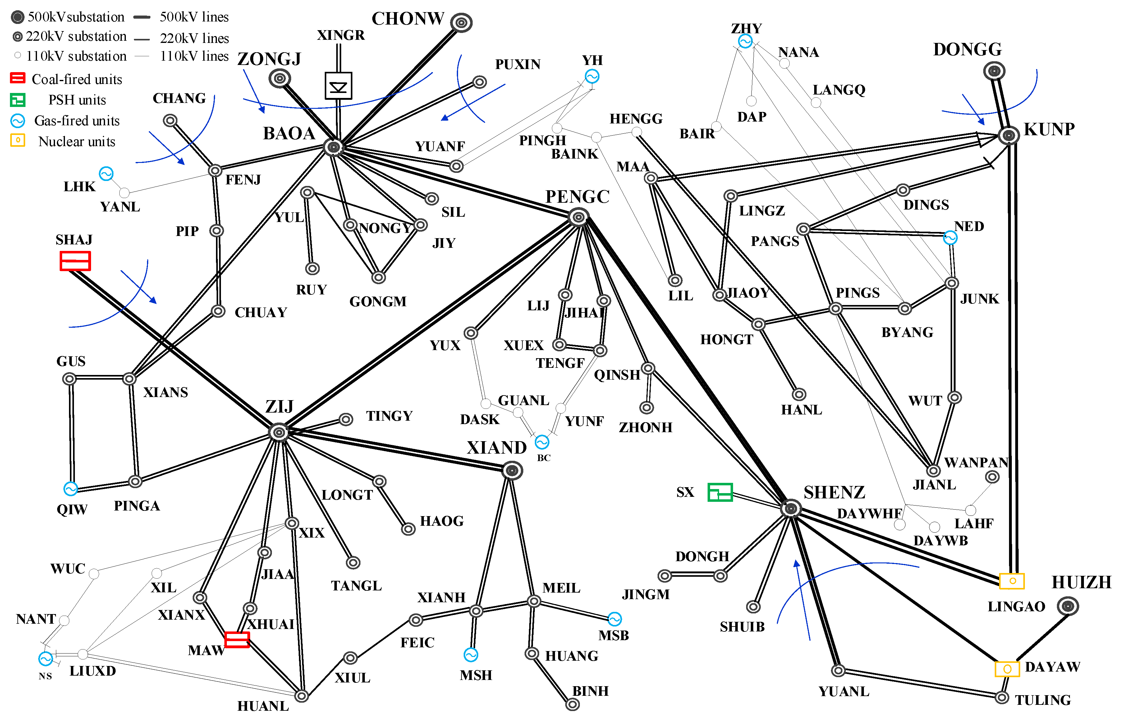
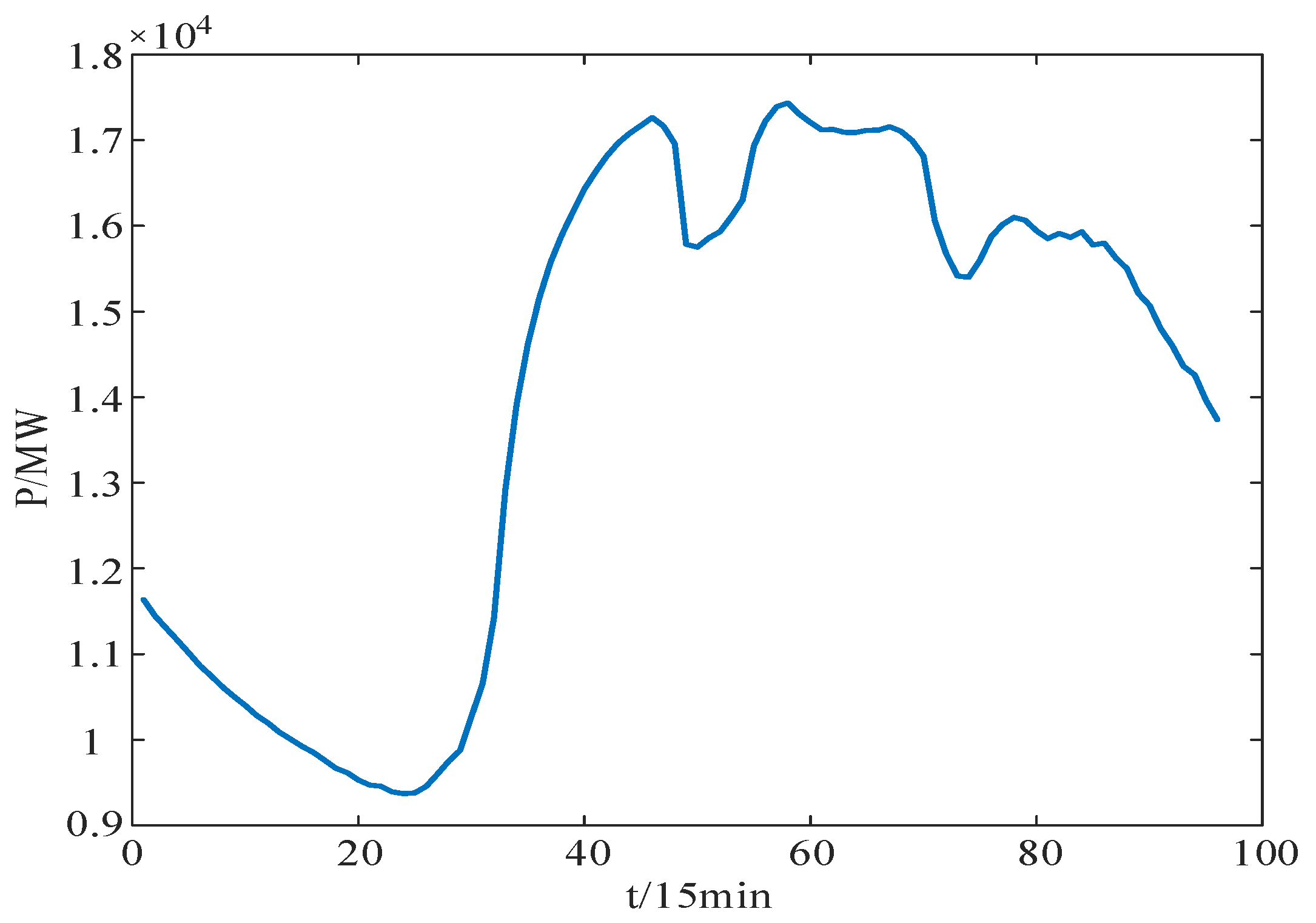
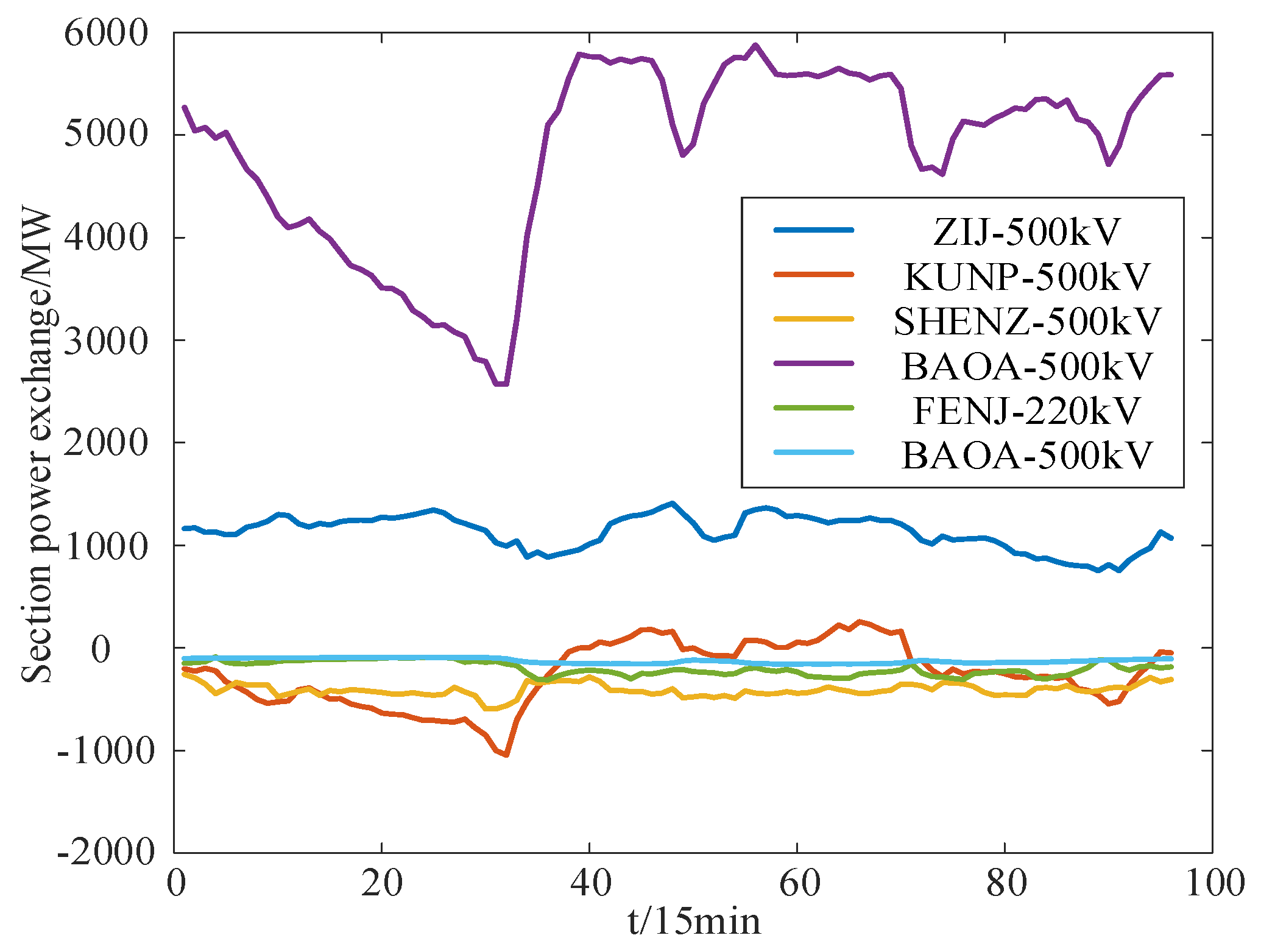
5.3. Shenzhen City Power Grid Including 110 kV Network

To fully demonstrate the computational efficiency of the relaxed QAPF model in the SCUC problem of a large-scale regional grid, another case of the Shenzhen city power grid including a 110-kV network is studied. In the grid, there are 1560 buses and 1757 branches, including 1028 transformer branches and 729 transmission lines. The X/R ratios of 110-kV transmission lines are in the range of 1.59–7.50, which does not satisfy the premise of R << X in the DCPF model. The system consists of 38 thermal units (including six coal-fired and 32 gas-fired), four nuclear units, and two PSH units. Parameters of several units are listed in Table 9. The values of Es,min, Es,max and Es,0 are 440 MWh, 4328 MWh and 846 MWh. The two PSH units store the water in the same upper reservoir. There are six power interchange sections connected to outside systems. The topology of the main network including several generators connected to the 110-kV network is shown in Figure 13. The forecast total load curve of the system is shown in Figure 14. In China, various city regional grids are attributed to the upper provincial grid. The interchange power schedule between different neighboring city regional grids is determined by the operators of the upper provincial grid so that the security constraints and economic benefits of different regional grids can be coordinated. Therefore, for the SCUC problem of a city regional grid, the power schedules of interchange sections with the external grids need to be determined by the upper provincial grid and given at first. The power schedules of six interchange sections at each time interval are shown in Figure 15. The used data is the actual data of August 21, 2017. There are 26 key transmission sections that are considered in the network security constraints, and the security limits of 10 key transmission sections are listed in Table 10. Lu% and Ld% are set as 3% and 1%, respectively.

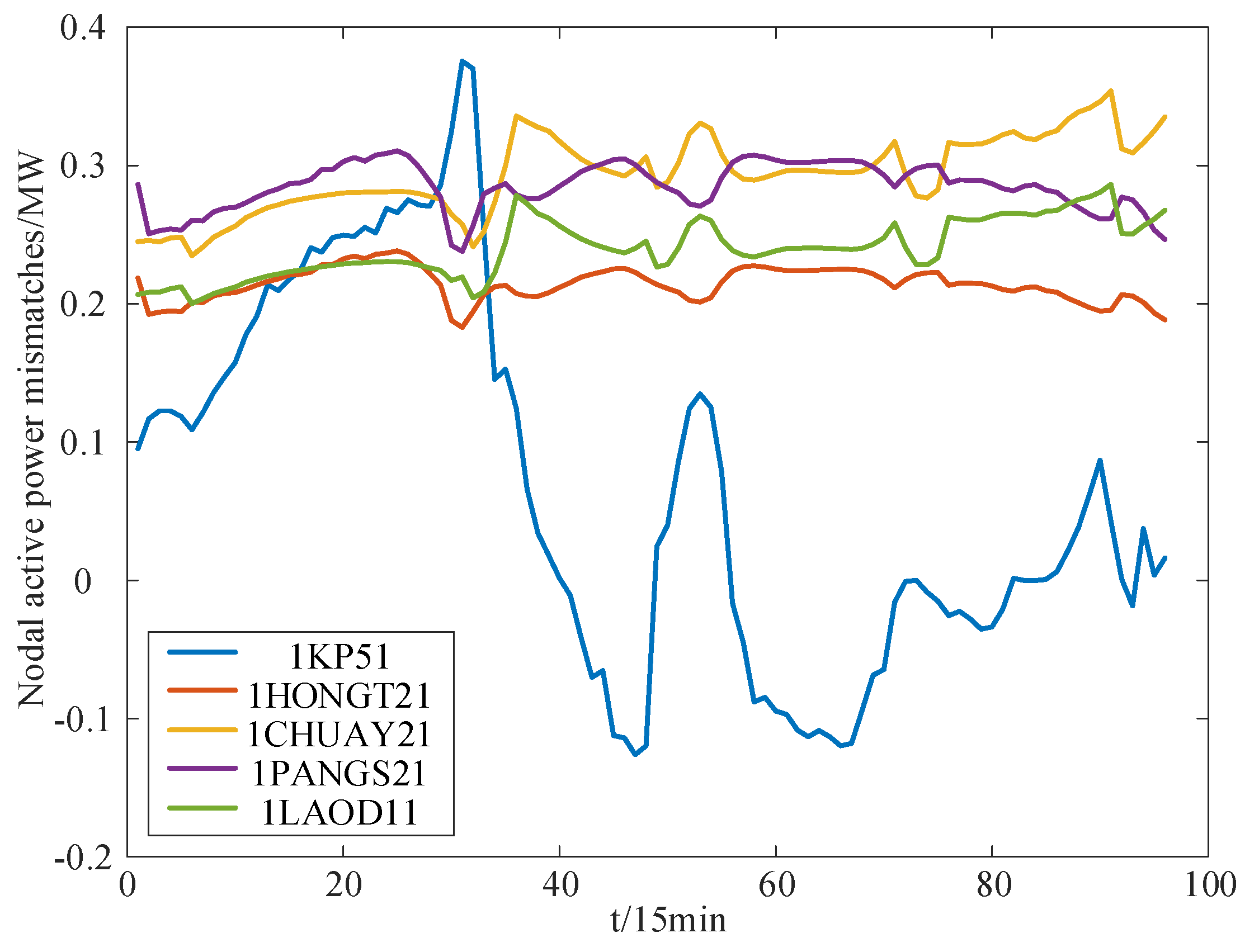
5.3.1. Precision Analysis of QAPF Model in Computing the Active Power of Lines

The QAPF model and common DCPF model are applied to compute the active power of lines, and the results are compared with those of the ACPF model in Table 11. It can be observed that the maximum relative deviation of the active power of lines computed by the DCPF model is greater than 20%, whereas the maximum relative deviation of the active power of lines computed by the QAPF model is less than 5%, which is more accurate. Therefore, the proposed QAPF model is more suitable for computing the active power of lines of power systems including 110 kV networks.

5.3.2. Precision Analysis of SCUC Models with Different PF Models

The CPLEX, DICOPT, and GUROBI solvers in the GAMS software are used to solve the SCUC problem based on the DCPF model (MILP model), the QAPF model (MINNP model), and the relaxed QAPF model (MICP model), respectively, and the objective values and calculation times are listed in Table 13. The active power of lines computed by the DCPF model has great deviation, which may cause the network constraints to be too strict and lead to the more frequent startup/shutdown of units, consequently increasing the total operating cost. From Table 12, the computation time of the MILP model is the shortest, but the accuracy is also the lowest. The MICP and MINNP models perform similarly in terms of accuracy, but the MICP model can be solved with high efficiency, since in large-scale optimization problems, the calculation efficiency of convex programming is higher, indicating that the proposed MICP model has great advantages when solving large-scale SCUC models.
To further demonstrate the advantages of the convex-hull relaxation of the QAPF model, the data of several other days (i.e., August 16–21, 2017) are substituted into the three SCUC models, with the results shown in Table 13. When the data are from August 17 and 20, the MINNP model cannot reach a converged solution, whereas the MICP model can still obtain an optimal solution. Regarding the data of other days, the calculation time of the MICP model is obviously less than that of the MINNP model. These results demonstrate that the proposed MICP model after the convex-hull relaxation of the QAPF model has higher calculation reliability and efficiency than the original MINNP model.
To verify whether the convex hull relaxation constraints are accurate to the original quadratic equalities, the deviation between the two sides of quadratic equality (25) is computed for different branches from the data of August 18, and the absolute deviations of five lines are shown in Figure 16. It can be seen that the maximum absolute deviation is less than 0.045 MW, indicating that the obtained active power of lines is very close to satisfying the original quadratic equality constraints. The maximum nodal active power mismatches of all the buses are less than 0.4MW, which is quite small when compared with the nodal active power, as shown in Figure 17. The results demonstrate that the proposed MICP model after the convex hull relaxation is accurate for the original MINNP model.
The active power output schedules of coal-fired thermal units, gas-fired thermal units, and PSH units are shown in Figure 18, Figure 19 and Figure 20. The coal-fired units operate at their upper limit of power output in most of the time intervals, since for coal-fired units, the start-up/shut-down costs are much higher, the minimum on-off time periods are much longer, and the ramping rates are small, therefore, their regulation flexibility is low. However, the gas-fired units have lower start-up/shut-down costs, shorter minimum on-off time periods, and larger ramping rates; therefore, gas-fired units can regulate their power output more frequently to accommodate the fluctuation of daily load. In addition, the PSH units can flexibly regulate the operational modes and power output according to the load fluctuation. When the load is heavy in the day, the PSH units tend to generate; when the load is low in the night, the PSH units tend to pump. This allows the PSH units to shave the peaks and filling valleys of the load curve. The total stored energy schedule in the upper reservoir of PSH units is shown in Figure 21. It can be seen that the stored energy is always within the maximum and minimum limit.
The optimal dispatch results when the SR capacity of the PSH units is considered in the constraint of the system SR capacity requirement and when it is not considered are compared, as shown in Table 14. When the system SR capacity requirement is the same, the optimal dispatch solution that considers the SR capacity of the PSH units can get a lower total operating cost. Although the thermal units need to start or stop more frequently and therefore increase the start-up/shut-down costs, the operation cost of the thermal units decreases evidently, resulting in the decrease of total cost. It is demonstrated that when the SR capacity of the PSH units is considered, the SR capacity of the thermal units can be reduced; therefore, some thermal units can be shut down to save the fuel cost, and it can enable the other thermal units to operate at a lower cost state. Hence, the economics of the system operation can be improved. When the load uncertainty, that is, the positive and negative SR capacity ratios, increase, the percentage decrease of total cost when considering the SR capacity of PSH units increases, indicating that when the load uncertainty is high, the reduction of the total cost will be more apparent.

6. Conclusions

An MICP algorithm for SCUC of a power system with a 110-kV network and PSH units is proposed. Based on the results of the case studies on the IEEE-9 bus system, the PEGASE 89 bus system and the Shenzhen city power grid including a 110-kV network, the following conclusions can be proposed:
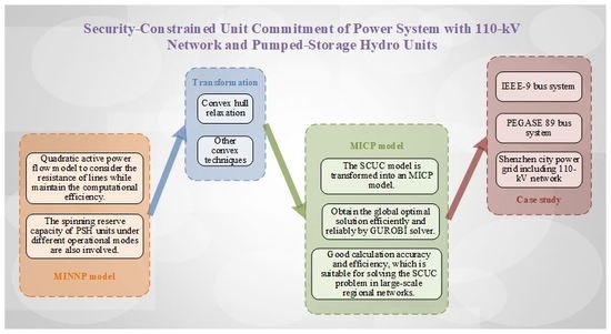
  • For a power system including a 110-kV network, the DCPF model cannot compute the active power of lines accurately, and the proposed QAPF model considering the resistance of lines can improve the calculation accuracy effectively;
  • The convex hull relaxation can be applied to transform the SCUC problem with QAPF constraints from an MINNP model into an MICP model, which has faster computation efficiency and higher accuracy in solving the SCUC problem of large-scale regional power grids;
  • By considering the SR capacity of PSH units in the SCUC model, the SR capacity required by thermal units can be reduced, which enables the thermal units to operate at a state in which the fuel costs are more economic and the total operation cost of the system can be decreased.
For future work, the research can be enhanced from the following aspects: (1) In this research, only the network security constraints in the normal operation state (the structure of the power grid is complete) are included in the formulation. To make the proposed model more suitable for practical operation, the network security constraints under N-1 contingencies may be added into the model, and the method of solving the large-scale SCUC model including multiple N-1 contingencies’ security constraints in an actual power grid may be developed. (2) Various kinds of SR such as primary and secondary SR capacities becoming common in actual operation, and the development of electricity market needs to specify different kinds of SR. Therefore, it’s necessary to consider different kinds of SR capacity in the model.

Author Contributions

Formal analysis, G.F.; Investigation, Y.L. (Yuan Lu); Methodology, S.L., G.F. and Q.L.; Supervision, S.L., M.L. and Y.L. (Yi Lu); Writing—review & editing, G.F.

Funding

This research was funded by the National Natural Science Foundation of China (grant no. 51977080), the Fundamental Research Funds for the Central Universities of China (2019MS015) and the Science and Technology Project of Shenzhen Power Supply Bureau Co., Ltd. (SZKJXM20160174).

Acknowledgments

The authors gratefully acknowledge the support of the National Natural Science Foundation of China, the Fundamental Research Funds for the Central Universities of China and the Science and Technology Project of Shenzhen Power Supply Bureau.

Conflicts of Interest

The authors declare no conflict of interest.

References

  1. Ruzic, S.; Rajakovic, N. A new approach for solving extended unit commitment problem. IEEE Trans. Power Syst. 1991, 6, 269–277. [Google Scholar] [CrossRef]
  2. Khodaei, A.; Shahidehpour, M. Transmission switching in security-constrained unit commitment. IEEE Trans. Power Syst. 2010, 25, 1937–1945. [Google Scholar] [CrossRef]
  3. Fu, Y.; Shahidehpour, M. Fast SCUC for large-scale power systems. IEEE Trans. Power Syst. 2007, 22, 2144–2151. [Google Scholar] [CrossRef]
  4. Ahmadi, H.; Ghasemi, H. Security-constrained unit commitment with linearized system frequency limit constraints. IEEE Trans. Power Syst. 2014, 29, 1536–1545. [Google Scholar] [CrossRef]
  5. Gutierrez-Alcaraz, G.; Hinojosa, V.H. Using generalized generation distribution factors in a MILP model to solve the transmission-constrained unit commitment problem. Energies 2018, 30, 2232. [Google Scholar] [CrossRef]
  6. Bai, Y.; Zhong, H.W.; Xia, Q.; Kang, C.Q.; Xie, L. A decomposition method for network-constrained unit commitment with AC power flow constraints. Energy 2015, 88, 595–603. [Google Scholar] [CrossRef]
  7. Castillo, A.; Laird, C.; Silva-Monroy, C.A.; Watson, J.P.; O’Neill, R.P. The unit commitment problem with AC optimal power flow constraints. IEEE Trans. Power Syst. 2016, 31, 4853–4866. [Google Scholar] [CrossRef]
  8. Wang, C.; Fu, Y. Fully parallel stochastic security-constrained unit commitment. IEEE Trans. Power Syst. 2016, 31, 3561–3571. [Google Scholar] [CrossRef]
  9. Liu, J.; Laird, C.D.; Scott, J.K.; Watson, J.; Castillo, A. Global solution strategies for the network-constrained unit commitment problem with AC transmission constraints. IEEE Trans. Power Syst. 2019, 34, 1139–1150. [Google Scholar] [CrossRef]
  10. Yuan, H.Y.; Li, F.X.; Wei, Y.L.; Zhu, J.X. Novel linearized power flow and linearized OPF models for active distribution networks with application in distribution LMP. IEEE Trans. Smart Grid 2018, 9, 438–448. [Google Scholar] [CrossRef]
  11. Nasri, A.; Kazempour, S.J.; Conejo, A.J.; Ghandhari, M. Network-constrained AC unit commitment under uncertainty: A Benders’ decomposition approach. IEEE Trans. Power Syst. 2016, 31, 412–422. [Google Scholar] [CrossRef]
  12. Amjady, N.; Dehghan, S.; Attarha, A.; Conejo, A.J. Adaptive robust network-constrained AC unit commitment. IEEE Trans. Power Syst. 2017, 32, 672–683. [Google Scholar] [CrossRef]
  13. Aghaei, J.; Nikoobakht, A.; Siano, P.; Nayeripour, M.; Heidari, A.; Mardaneh, M. Exploring the reliability effects on the short term AC security-constrained unit commitment: A stochastic evaluation. Energy 2016, 114, 1016–1032. [Google Scholar] [CrossRef]
  14. Nikoobakhtm, A.; Mardaneh, M.; Aghaei, J.; Guerrero-Mestre, V.; Contreras, J. Flexible power system operation accommodating uncertain wind power generation using transmission topology control: An improved linearised AC SCUC model. IET Gener. Transm. Distrib. 2017, 11, 142–153. [Google Scholar] [CrossRef]
  15. Khodayar, M.E.; Shahidehpour, M.; Wu, L. Enhancing the dispatchability of variable wind generation by coordination with pumped-storage hydro units in stochastic power systems. IEEE Trans. Power Syst. 2013, 28, 2808–2818. [Google Scholar] [CrossRef]
  16. Khodayar, M.E.; Abreu, L.; Shahidehpour, M. Transmission-constrained intrahour coordination of wind and pumped-storage hydro units. IET Gener. Transm. Distrib. 2013, 7, 755–765. [Google Scholar] [CrossRef]
  17. Lin, S.J.; Liu, M.B.; Li, Q.F.; Lu, W.T.; Yan, Y.; Liu, C.P. Normalised normal constraint algorithm applied to multi-objective security-constrained optimal generation dispatch of large-scale power systems with wind farms and pumped-storage hydroelectric stations. IET Gener. Transm. Distrib. 2017, 11, 1539–1548. [Google Scholar] [CrossRef]
  18. Varkani, A.K.; Daraeepour, A.; Monsef, H. A new self-scheduling strategy for integrated operation of wind and pumped–storage power plants in power markets. Appl. Energy 2011, 88, 5002–5012. [Google Scholar] [CrossRef]
  19. Kumano, J.; Yokoyama, A. Optimal weekly operation scheduling on pumped storage hydro power plant and storage battery considering reserve margin with a large penetration of renewable energy. In Proceedings of the 2014 International Conference on Power System Technology, Chengdu, China, 20–22 October 2014; pp. 1120–1126. [Google Scholar]
  20. Xiong, P.; Jirutitijaroen, P. Stochastic unit commitment using multi–cut decomposition algorithm with partial aggregation. In Proceedings of the 2011 IEEE Power and Energy Society General Meeting, Detroit, MI, USA, 24–28 July 2011; pp. 1–8. [Google Scholar]
  21. Zhao, C.Y.; Guan, Y.P. Unified stochastic and robust unit commitment. IEEE Trans. Power Syst. 2013, 28, 3353–3361. [Google Scholar] [CrossRef]
  22. Hedman, K.W.; Ferris, M.C.; O’Neill, R.P.; Fisher, E.B.; Oren, S.S. Co–optimization of generation unit commitment and transmission switching with N–1 reliability. IEEE Trans. Power Syst. 2010, 25, 1052–1063. [Google Scholar] [CrossRef]
  23. Jabr, R.A.; Singh, R.; Pal, B.C. Minimum loss network reconfiguration using mixed-integer convex programming. IEEE Trans. Power Syst. 2012, 27, 1106–1115. [Google Scholar] [CrossRef]
  24. Li, Q.F.; Yu, S.; Al–Sumaiti, A.; Turitsyn, K. Micro water–energy nexus: Optimal demandside management and quasi-convex hull relaxation. IEEE Trans. Control Netw. Syst. 2018. [Google Scholar] [CrossRef]
  25. Li, Q.F.; Vittal, V. The convex hull of the AC power flow equations in rectangular coordinates. In Proceedings of the 2016 IEEE Power and Energy Society General Meeting (PESGM), Boston, MA, USA, 17–21 July 2016; pp. 1–5. [Google Scholar]
  26. Li, Q.F.; Vittal, V. Convex Hull of the Quadratic Branch AC Power Flow Equations and Its Application in Radial Distribution Networks. IEEE Trans. Power Syst. 2018, 33, 839–850. [Google Scholar] [CrossRef]
  27. Available online: https://www.gams.com/latest/docs/UG_MAIN.html (accessed on 19 September 2019).
  28. Josz, C.; Fliscounakis, S.; Maeght, J.; Panciatici, P. AC power flow data in MATPOWER and QCQP format: iTesla, RTE snapshots, and PEGASE. arXiv 2016, arXiv:1603.01533. [Google Scholar]
  29. Fliscounakis, S.; Panciatici, P.; Capitanescu, F.; Wehenkel, L. Contingency ranking with respect to overloads in very large power systems taking into account uncertainty, preventive and corrective actions. IEEE Trans. Power Syst. 2013, 28, 4909–4917. [Google Scholar] [CrossRef]
Figure 1. Piece-wise linearization of generation cost function.
Energies 12 03646 g001
Figure 2. Convex hull of the quadratic equality.
Energies 12 03646 g002
Figure 3. Structure diagram of IEEE-9 bus system.
Energies 12 03646 g003
Figure 4. Forecast total load curve.
Energies 12 03646 g004
Figure 5. Optimal dispatch scheduling of units computed by three different SCUC models.
Energies 12 03646 g005
Figure 6. Stored energy schedule in the upper reservoir of PSH unit by three different SCUC models.
Energies 12 03646 g006
Figure 7. Absolute deviation between the values of the two sides of quadratic equality (25) on different lines.
Energies 12 03646 g007
Figure 8. The nodal active power mismatches of different buses.
Energies 12 03646 g008
Figure 9. Absolute deviation between the values of the two sides of quadratic equality (25) on different lines.
Energies 12 03646 g009
Figure 10. The five maximum nodal active power mismatches of different buses.
Energies 12 03646 g010
Figure 11. Active power output schedule of several gas-fired thermal units and PSH units.
Energies 12 03646 g011
Figure 12. Stored energy schedule in the upper reservoir of PSH unit.
Energies 12 03646 g012
Figure 13. Topology of the main network including several units of 110-kV.
Energies 12 03646 g013
Figure 14. Forecast total load curve of the system.
Energies 12 03646 g014
Figure 15. Power scheduling of interchange sections with outside systems.
Energies 12 03646 g015
Figure 16. Absolute deviation of the two sides of quadratic equality (25) of several branches.
Energies 12 03646 g016
Figure 17. The five maximum nodal active power mismatches of different buses.
Energies 12 03646 g017
Figure 18. Active power output schedule of coal-fired units.
Energies 12 03646 g018
Figure 19. Active power output schedule of gas-fired units.
Energies 12 03646 g019
Figure 20. Active power output schedule of PSH units.
Energies 12 03646 g020
Figure 21. Stored energy schedule in the upper reservoir of PSH units.
Energies 12 03646 g021
Table 1. Power value of each phase of the load buses (kW, kvar).
LinesResistance/ΩReactance/ΩSusceptance/10−4SRatio X/RPl,max/MW
Bus-8----Bus-710.117185.69801.25188.47250
Bus-8----Bus-914.1640119.97721.75598.47150
Bus-5----Bus-738.0880191.63032.57095.03120
Bus-6----Bus-946.4198202.34253.00784.36150
Bus-4----Bus-511.9025101.17231.47898.50250
Bus-4----Bus-620.2343109.50301.32755.41250
Table 2. Parameters of the generation units.
Unit TypeBusUpper/Lower Limits (MW)Ramping Up/Down Limits (MW/min) Fuel-Cost Coefficients Of Thermal UnitsMinimum On/Off PeriodsStart-Up/Shut-Down Cost (103 ¥)
Ai,2 (¥/MW2h))Ai,1 (¥/(MWh))Ai,0 (¥/h)
Thermal2150/501.20.0272702759.402/3400/100
3220/1201.20.0272702759.403/4500/100
PSH1100/−100200001/180/40
Table 3. Results by different power flow models.
LinesDCPF/p.u.QAPF/p.u.ACPF/p.u.Relative Deviation of DCPF/%Relative Deviation of QAPF/%
BUS-4----BUS-60.243870.185980.1948225.184.54
BUS-5----BUS-71.356131.298851.289535.160.72
BUS-6----BUS-91.143871.086591.095894.380.85
BUS-8----BUS-70.643870.638930.647770.601.36
BUS-8----BUS-90.356130.361070.352231.112.51
Table 4. Comparison of the results.
SCUC ModelObjective Value/103 ¥Start-Up/Shut-Down Cost/103 ¥Fuel Cost/103 ¥CPU Time/s
MILP8878.097208158.092.3
MINNP8391.252408151.2510.8
MICP8392.382408152.389.4
Table 5. Parameters of generator units.
Unit TypeBus NumberUpper/Lower Limits (MW)Ramping Up/Down Limits (MW/min)Fuel-Cost Coefficients of Thermal Units Ai,1/(¥/(MWh))Minimum On/Off PeriodsStart-Up/Shut-Down Cost (103 ¥)
PSH1666/-66666.7-1/112/5
Gas-fired21500/5008.363232/260/25
3500/166.72.860001/120/8
42000/666.71163232/240/18
5100/-727.66.760001/122/10
621.23/7.081.350001/18/3
71200/4007.363231/140/20
8100/-908.938.363231/140/18
9600/2003.380001/120/8
10600/2003.380001/120/8
11600/2003.380001/120/8
Table 6. The X/R ratio of the lines of the PEGASE 89 bus system.
X/R RatioPercentage/%
0–630.4
6–1238.6
>1231.0
Table 7. Comparison of the active power of several lines computed by different power flow models.
LinesDCPF/p.u.QAPF/p.u.ACPF/p.u.Relative Deviation of DCPF/%Relative Deviation of QAPF/%
29-620.72800.73020.73691.210.91
10-222.84492.87652.97624.413.35
26-84.37144.47294.67506.494.32
75-742.13982.14782.12470.711.09
52-230.35270.29250.278726.554.95
85-621.21551.23651.28125.133.49
60-302.08662.09612.18754.614.36
4-414.32514.32904.47693.393.30
36-780.70120.72980.76207.984.23
59-794.48574.47214.59292.332.63
Table 8. Comparison of results computed by three SCUC models.
Model TypeObjective Value/103 ¥Start-Up/Shut-Down Cost/103 ¥Fuel Cost/103 ¥Time/s
MILP9131.744978634.7417.48
MINNP9112.924618651.92477.96
MICP9112.104618651.10225.11
Table 9. Parameters of several units.
Unit TypeBusUpper/Lower Limits (MW)Ramping Up/Down Limits (MW/min) Fuel-Cost Coefficients Of Thermal UnitsMinimum On/Off PeriodsStart-Up/Shut-Down Cost (103 ¥)
Ai,2/(¥/MW2h))Ai,1/(¥/(MWh))Ai,0/(¥/h)
Coal-fired thermalMAW1320/1804.50.027270919896/12800/180
MAW3330/1804.50.027279919896/12800/180
MAW6330/1804.50.027279919896/12800/180
Gas-fired thermalQIW1370/24016.7-582.35-2/2150/50
MSH7120/10016.7-722.99-2/2100/50
NED1370/24016.7-582.35-2/2105/34.39
NSg1120/955.715-722.99-2/1100/50
BCg5132/10010-722.99-2/1105/55
ZHYg4156/12010-722.99-2/130/25
YHg1124/9510-722.99-2/1100/30
PSHSXg1306/−324999---1/180/40
SXg2306/−324999---1/180/40
Table 10. Security limits of several key transmission sections.
Transmission SectionsLines in the SectionsSecurity Limit Power (MW)
1LINGKUN-I, II + PENGSHEN-I, II2600
2LINGSHEN-I, II2900
3SHAJING-I, II3400
4ANFEN-I, II1150
5ANXIANG-I, II1150
6JINGTING-I, II1020
7PENGJI-I, II920
8LINGKUN-I, II+HEHUI2000
9KUNDING-I, II+JIAOHONG-I, II1280
10JINGXIAN-I, II+JINGLONG-I, II1300
Table 11. Comparison of the active power of several lines computed by different PF models.
LinesDCPF/p.u.QAPF/p.u.ACPF/p.u.Relative Deviation of DCPF/%Relative Deviation of QAPF /%
PENGC-SHENZ3.91374.31044.29008.770.48
PENGC-QINSH4.66724.71294.71250.960.01
SHENZ-SX4.10024.08944.09130.220.05
ZIJ-XIX0.20900.27500.268622.192.39
BAOA-PENGC18.861720.713620.95679.991.16
MAAO-JIAOY0.97381.07481.129013.754.80
FENJ-PIPA3.33593.45473.50744.891.50
XIX-WUC0.07910.06920.068814.950.65
HUANL-XIUL2.98913.00643.00750.610.04
HUANG-BINH4.79304.81614.81850.530.05
Table 12. Comparison of results computed by three SCUC models.
Model TypeObjective Value/103 ¥Start-Up/Shut-Down Cost/103 ¥Fuel Cost/103 ¥Time/s
MILP42,492.873644.7838,848.09930
MINNP40,974.042140.1538,833.8921,098
MICP40,997.572179.1738,818.4010,509
Table 13. Results from several days’ data by three SCUC models.
DateModel TypeObjective Value/103 ¥Time/sSolution Status
Aug. 16MILP31,996.17892Converged
MINNP31,022.5722,893Converged
MICP31,021.5910,335Converged
Aug. 17MILP35,896.17932Converged
MINNP--Not converged
MICP35,391.2410,127Converged
Aug. 18MILP35,691.06879Converged
MINNP35,162.0122,980Converged
MICP35,165.0410,628Converged
Aug. 19MILP33,892.81899Converged
MINNP33,274.8923,890Converged
MICP33,272.7010,522Converged
Aug. 20MILP31,293.23882Converged
MINNP--Not converged
MICP30,892.2310,267Converged
Aug. 21MILP42,492.87930Converged
MINNP40,994.0421,098Converged
MICP40,997.5710,509Converged
Table 14. Comparison of the results when the PSH units’ spinning reserve is considered or not considered.
Ratio of SR Capacity RequirementWhether SR Capacity of PSH Units are ConsideredTotal Costs/103 ¥Relative Reduction of Total Cost/%Operation Costs of Thermal Units/103 ¥Start-Up/Shut-Down Costs of Thermal Units/103 ¥
Lu% = 3%, Ld% = 1%YES41579.270.5738839.492499.78
NO41816.7039795.531781.17
Lu% = 4%, Ld% = 2%YES42758.143.2239272.973245.17
NO44133.0641023.282869.78
Lu% = 5%, Ld% = 3%YES44413.605.4940122.824050.78
NO46853.9143101.353512.56

