Article

Coordinated Control in VSC-HVDC Multi-Terminal Systems to Improve Transient Stability: The Impact of Communication Latency

Instituto de Investigación Tecnológica (IIT), ETSI ICAI, Universidad Pontificia Comillas, Madrid 28015, Spain
*
Author to whom correspondence should be addressed.
Energies 2019, 12(19), 3638; https://doi.org/10.3390/en12193638
Submission received: 31 July 2019 / Revised: 15 September 2019 / Accepted: 19 September 2019 / Published: 24 September 2019
(This article belongs to the Special Issue HVDC/FACTS for Grid Services in Electric Power Systems)

Abstract

:
Power transmission is the main purpose of high voltage direct current systems based on voltage source converters (VSC-HVDC). Nevertheless, this type of system can also help to improve transient stability by implementing suitable supplementary controllers. Previous work proposed active- (P) and reactive-power (Q) control strategies in VSC-HVDC multi-terminal systems (VSC-MTDC, for short) to improve transient stability, producing significant improvements. In those strategies, each VSC station of the MTDC system compares its frequency measurement with the average of the frequencies measured by all converter stations of the MTDC system (weighted-average frequency, WAF) in order to modulate its own P and Q injections. Hence, a communication system is required. This paper presents a detailed analysis of the impact of communication latency on the performance of those control strategies. The communication delays have been modelled using a Padé’s approximation and their impact on the performance of the control strategies have been assessed by means of time-domain simulation in PSS/E. The effect of the control strategies on transient stability has been quantified with the critical clearing time (CCT) of a set of faults. Results show that the control strategies analysed present good results for realistic values of communication delays.

Graphical Abstract

1. Introduction

The main applications of high voltage direct current (HVDC) systems are: (a) transmission of large amounts of power over long overhead lines; (b) power transmission over middle-to-long isolated cables (underground or submarine cables); and (c) interconnection of asynchronous power systems. These characteristics make HVDC a key facilitating technology in several scenarios of present and future power systems. For example, almost all electrical energy systems around the world are being urged to integrate an ever-increasing number of renewable resources which are often in remote sites and will require power transmission over long distances. Hence, grid reinforcement with HVDC links is already in place in many locations and it is an attractive alternative of high voltage alternating current (HVAC) transmission in many others [1]. Furthermore, there is a conceptual proposal for building a pan-European multi-terminal HVDC grid (the so-called “supergrid”) interconnecting several countries and connecting offshore wind energy from the North Sea [2,3,4,5]. This “supergrid” would be connected at different points to the conventional HVAC transmission system. Undoubtly, the most appropriate technology for a multi-terminal HVDC system is the one based on voltage source converters (VSC-HVDC), which has several advantages for certain applications, in comparison with the classic line commutated converter technology based on thyristors (LCC-HVDC) [1].
Key aspects for the deployment of multi-terminal VSC-HVDC grids are converter technology, control of the voltage of the HVDC grid, HVDC breakers and HVDC protection strategies. The most recent converter technology for VSC-HVDC systems is the so-called modular multi-level converter (MMC) [6,7], which makes it possible to obtain output AC voltages with a very-low harmonic content. For example, MMC technology is already being used in the VSC-HVDC interconnector between France and Spain through the Catalonian Pyrenees (INELFE) [8]. DC-voltage control in VSC-HVDC multi-terminal systems must always be guaranteed and there are different control alternatives [9,10]. It can be classified into: (a) centralised DC-voltage control; and (b) distributed DC-voltage control (with local DC-voltage droop control). In the former, only one converter controls the DC voltage (the DC slack), while in the latter approach, DC-voltage control is shared among the converters [11,12] and it is more suitable for large VSC-MTDC systems. There are also more advanced distributed DC-voltage control strategies, aiming to improve the accuracy in power sharing: the so-called pilot-voltage droop control [13], which uses global measurements and a recent control approach based on a power sharing index [14], in which each converter uses measurements of a nearby converter. VSC-HVDC grids need HVDC breakers to be capable to isolate faults in the HVDC grid, while maintaning the system in operation. The interruption of the current in DC is much more difficult than the interrumption of the current in AC, since the former does not pass through zero. Furthermore, HVDC breakers need to open the circuit in a few milliseconds, in order to protect the converters. The main manufacturers already have prototypes for HVDC breakers [15,16], although the technology is not mature yet. VSC-HVDC systems also need effective protection algorithms to detect and locate faults in the HVDC grid within milliseconds. Different protection algorithms for VSC-HVDC grids have been proposed recently [17,18,19,20,21,22,23,24,25].
VSC-HVDC systems are very expensive and, although their main purpose will always be to facilitate power transmission overcoming the limitations of traditional HVAC systems, any additional contribution to the control and operation of power systems should be welcome. For example, several publications have already explored control strategies in point-to-point VSC-HVDC links to improve transient stability of power systems [26,27,28,29]. Transient stability (angle stability against large disturbances [30]) margins deteriorate seriosly when long and heavily loaded HVAC lines are used. In multi-machine systems, transient stability is a global problem involving synchronism of all generators of the system and the most effective control actions to improve those margins use global measurements, such as the speed of the centre of inertia (COI) of the system [31,32,33].
Recently, several control strategies for multi-terminal VSC-HVDC systems (VSC-MTDC, for short) have been proposed to improve transient stability. A supplementary control strategy for active- (P) and reactive-power (Q) injections of the VSC stations, using a linear combination of the speed deviations of the generators of the system as input signal, was proposed in [34]. The work in [35] proposed a bang-bang-type supplementary P controller at each VSC station, using a combination of the speed deviations of all generators of the system with respect to the speed of the COI as input signal. A sliding-mode control strategy for P injections in VSC-MTDC systems, also using the speed of the COI, was proposed in [36]. The speed of the COI for P and Q modulation in VSC-MTDC systems is also used in the control strategy proposed in [37]. All these control strategies require a Wide Area Measurement System (WAMS), so that each VSC can know the speeds of all generators of the system in real time. Alternatively, the work in [38] proposed a control strategy for P injections of converter stations in VSC-MTDC systems using the average of the frequencies measured at the connection point of the VSC stations (weighted-average frequency, or WAF for short), to improve transient stability. This strategy will be referred to as P-WAF in the rest of the paper. Similarly, the WAF was used to modulate Q injections at the converter stations in VSC-MTDC systems in [39] (strategy Q-WAF, for short), also to improve transient stability.
Although the speed of the COI seems to be the most comprehensive measurement to be used, strategies P-WAF and Q-WAF have two key advantages with respect this approach: each VSC station already measures the frequency at its AC terminals, for synchronisation purposes and a communication system within the VSC-MTDC system, only, is required.
Recent work has derived an analytical formula to approximate the bus frequencies as a linear combination of the speeds of all generators of the system [40], proving the idea that the speeds of the generators can be observed in the bus frequencies. In fact, the speed of the COI can also be approximated as a linear combination of a set of bus frequencies of the system [41].
Since control strategies P-WAF and Q-WAF require a communication system between the stations of the VSC-MTDC systems, their performance might be affected by communication latency. Previous work was restricted to prove that strategies P-WAF and Q-WAF could stand a reasonable communication latency. However, a detailed analysis of the impact of communication delays on these control strategies has not been reported in the literature so far. Along this line, the contributions of this paper include:
  • A comprehensive analysis of the impact of communication latency on strategies P-WAF (P injections of the VSC stations) and Q-WAF (Q injections of the VSC stations).
  • A comprehensive analysis of the impact of communication latency on simultaneous modulation of P and Q injections of the VSC stations by implementing strategies P-WAF and Q-WAF together (PQ-WAF, for short).
  • A detailed analysis of the impact of different tipes of communication delays on strategies P-WAF, Q-WAF and PQ-WAF.
  • Analysis of the impact of communication delays on strategy P-WAF, depending on the approach used for DC-voltage control in the VSC-MTDC system (a single DC-slack converter or DC-voltage droop control).
The rest of the paper is organised as follows. Section 2 describes a suitable model for VSC-MTDC systems for electro-mechanical simulation. Section 3 describes the proposed transient-stability-tailored control strategies in VSC-MTDC systems based on the WAF. Section 4 presents a small case study (Kundur’s two-area test system with an embedded VSC-MTDC system) to illustrate impact of communication latency on the performance of the control strategies. Section 5 presents the results of a larger case study (Cigré Nordic32A test system with an embedded VSC-MTDC system). Section 6 presents the conclusions of the paper. Finally, data of the case study are provide in Appendix A and Appendix B.

2. VSC-HVDC Multi-Terminal Systems

A VSC-MTDC system consists of several VSC stations connecting a DC grid to one or more AC grids. Figure 1 shows a hybrid AC/DC system with an embedded VSC-MTDC system while Figure 2 illustrates the dynamic model of a VSC station connected to an AC grid and to a DC grid, following the guidelines of [42,43] for electro-mechanical simulation. The guidelines of the modelling approach used are provided in this section, while details are available in [44].

2.1. VSC Stations

A VSC station is seen, from the AC side, as a voltage source ( e ¯ c , i ) connected through a connection impedance (reactor + transformer: z ¯ s , i = r s , i + j x s , i ) to the connection point (with voltage u ¯ s , i ) (Figure 2).
A VSC station is usually controlled with vector control, where mobile d q axes are aligned with the voltage of the connection point: u ¯ s , i = u s , i + j 0 . The control system has an inner current loop ( i s , d , i and i s , q , i ) and an outer control loop. Since, for transient stability studies, the dynamics of interest (transients spanning 1–20 s) are much slower than the dynamics of the inner controllers of the VSC stations, the closed loop of the inner current loops can be approximated by first-order transfer functions. Every VSC station has two degrees of freedom for the outer loop: (a) the converter can control either the active-power injection into the AC grid ( p s , i ) or the DC voltage ( u d c , i ) with the d-axis current; and (b) the converter can control either the reactive-power injection into the AC grid ( q s , i ) or the magnitude of the AC voltage at the connection point ( u s , i ) with the q-axis current. Operating limits of the converters can be easily implemented in the model [44].
AC and DC sides of a converter station are coupled by the energy conservation principle:
p c , i + p l o s s , i + p d c , i = 0
where losses, p l o s s , i , are best modelled as a quadratic function of the current injection of the VSC, i s , i (rms), as proposed in [45]:
p l o s s , i = a i + b i · i s , i + c i · i s , i 2

2.2. DC Grid

VSC stations are seen from the DC grid as current injections into the buses: i d c , i = p d c , i / u d c , i (Figure 2). DC lines are represented as lumped π models. Every DC branch i j will have the series resistance and the inductance of the DC line ( r d c , i j and L d c , i j , respectively). Every DC bus i will have an equivalent capacitance ( C d c , i ), that includes the equivalent capacitance of the DC side of the VSC station ( C V S C , i ) and the contribution of the shunt capacitance of the DC lines connected to that bus ( C c c , i j / 2 ):
C d c , i = C V S C , i + j i C c c , i j 2

2.3. Voltage Control in the DC Grid

Voltage control in the DC grid can be implemented either with a centralised approach (a single DC-slack converter) or with a distributed approach (DC-voltage droop control) [9,10]. In the DC-voltage droop approach, the active-power set point of every VSC station is given by [43]:
p s , i r e f = p s , i 0 1 k d c , i ( u d c , i 0 u d c , i )

2.4. Model Implementation

The dynamic model of a VSC-MTDC system has been implemented in PSS/E [46], following the guidelines of [47,48,49,50]. The initial operating point is obtained solving a sequential AC/DC power flow, as proposed in [51]. Details of the PSS/E implementation used for this work and its validation can be found in [44].

3. Control Strategies

Figure 3 shows a general diagram for P and Q control in a VSC station. In addition to the constant P set point required by the TSO ( p s 0 ) and the DC-voltage droop, the VSC station has a supplementary P set point ( Δ p s r e f ). Similarly, in addition to the constant Q set point ( p s 0 ), the VSC station has a supplementary Q set point ( Δ q s r e f ). Supplementary set points for P ( Δ p s r e f ) and Q injections ( Δ q s r e f ) are aimed to improve transient stability. Notice that the supplementary controllers could also be implemented with a centralised DC-voltage control in the VSC-MTDC without DC-voltage droop and only one converter looking after the DC voltage. Since voltage control in the HVDC grid is a major concern, any supplementary control strategy for P injections of the VSC stations in VSC-MTDC system must be compatible with the DC-voltage control scheme used.

3.1. Strategy P-WAF

The block diagram of P control of a VSC station, when using strategy P-WAF, is shown in Figure 4 [38]. A supplement proportional to the frequency error is added to the P set point. The frequency set point is calculated as the weighted average of the frequencies measured at the AC side of the VSC stations (weighted-averaged frequency, WAF):
ω * = ω ¯ = k = 1 n α k ω k , with α k [ 0 , 1 ] and k = 1 n α k = 1
where ω k is the frequency measured at the connection point of V S C k .
The controller consists of a proportional gain ( k P ), a low-pass filter for noise filtering (with time constant T f ), a wash-out filter in order to avoid the actuation of the controller under steady-state frequency deviations (with time constant T W ) and a saturation parameter ( Δ p m a x ). Notice that in Figure 4, the VSC has the DC-voltage droop control ( Δ p s r e f , D C ) implemented together with the supplementary control strategy, but this is not mandatory.
The performance of this control strategy can be summarised as follows:
  • If the frequency at the connection point of a VSC station is above the WAF, the converter will decrease its P injection into the AC grid, aiming to slow down nearby generators.
  • If the frequency at the connection point of a VSC station is below the WAF, the converter will increase its P injection into the AC grid, aiming to accelerate nearby generators.
  • This behaviour should pull together the angles of the generators of the system improving, therefore, transient stability.
The work in [38] proposed the following design of the controller gains ( k P , k ) and the weighting factors used to calculate the WAF ( α k ):
k P , k k P , T = α k , with k P , T = j = 1 n k P , j
This design ensures j = 1 n Δ p s , j r e f = 0 and avoids the interaction of the supplementary controller with the DC-voltage droop control.

3.2. Strategy Q-WAF

In strategy Q-WAF, a supplement proportional to the frequency error is added to the Q set point, as shown in Figure 5 [39]. The frequency set point is also calculated as the WAF (5). This controller also consists of a proportional gain ( k Q ), a low-pass filter (with time constant T f ), a wash-out filter (with time constant T W ) and a saturation parameter ( Δ q m a x ). Notice that strategy Q-WAF has an additional minus sign (Figure 5).
This control strategy can be summarised as follows:
  • If the frequency at the connection point of a VSC station is above the WAF, the converter will increase its Q injection into the AC grid, aiming to increase the electromagnetic torque applied to nearby generators and slow them down.
  • If the frequency at the connection point of a VSC station is below the WAF, the converter will decrease its Q injection into the AC grid, aiming to reduce the electromagnetic torque applied to nearby generators and accelerate them.
  • Again, this behaviour should eventually pull together the angles of the generators of the system, improving transient stability.
The following design was used in [39]:
k Q , k k Q , T = α k , k Q , T = j = 1 n k Q , j
This ensures j = 1 n Δ q s , j r e f = 0 . However, this condition is not mandatory for Q control.

3.3. Strategy PQ-WAF

P and Q injections of the VSC stations can be modulated simultaneously, according to strategies P-WAF (Figure 4) and Q-WAF (Figure 5), using the weighted-averaged frequency in Equation (5) as the frequency set point. This strategy will be named PQ-WAF in the rest of the paper.

3.4. Communication Latency

In strategies P-WAF, Q-WAF and PQ-WAF, every VSC station uses global signals of frequency measurements at the connection point of all the VSC stations of the VSC-MTDC system, in order to calculate the WAF in Equation (5). Hence, communications among the converter stations must be established and the calculation of the WAF will be subject to communication latency. For transient-stability-tailored controllers, fast communication systems are required (faster than 100 ms, in general). The work in [52] proposed a model to represent communication delays in wide-area control system. Total communication delay was divided into two parts: (a) the delay caused by the propagation of the information in the communication system; and (b) the operational delay, that accounts for the time required for the calculations. Total communication delays within the range 50–80 ms were reported in [52], according to phasor measurement unit (PMU) records in the Chinese power system and to real-time simulation experiments.
The impact of the communication latency on the performance of the proposed control strategies is analysed here by introducing a delay in the frequency at the AC bus of VSC station i, measured by VSC station j ( ω i j ):
ω i j = ω i e τ i j s
where τ i j accounts for the total communication delay (operational delay + communication delay). Hence, each VSC j will use a frequency set point for P and/or Q modulation ( ω j * in Figure 4 and Figure 5) using the delayed frequency measurements, according to:
ω j * = ω ¯ j = k = 1 n α k ω k j
The implementation of Equation (9) is shown in Figure 6.
The delay in Equation (8) has been implemented using a second-order Padé’s approximation [53]:
e τ i j s 1 τ i j 2 s + τ i j 2 12 s 2 1 + τ i j 2 s + τ i j 2 12 s 2

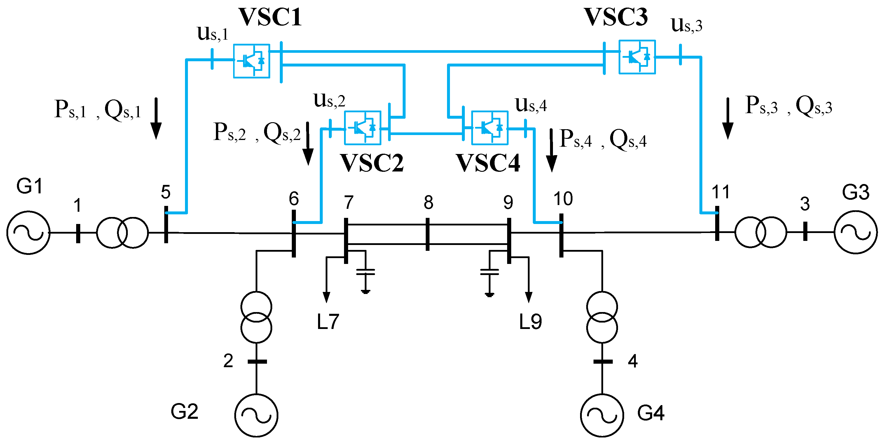
4. Case Study 1: Kundur’s Two-Area Test System with an Embedded VSC-MTDC System

The Kundur’s two-area test system [54] with an embedded 4-terminal VSC-MTDC system was used for simulation (Figure 7). Data are detailed in Appendix A. Converter stations were operated with DC-voltage droop control and reactive-power control. Simulations were carried out in PSS/E software [46], with the VSC-MTDC model presented in [44].
The initial operating point of the VSC-MTDC system was calculated running an AC/DC power flow, with the following specified variables:
  • VSC1: P s , 1 0 = 200 MW and Q s , 1 0 = 0 MVAr.
  • VSC2: P s , 2 0 = 200 MW and Q s , 2 0 = 0 MVAr.
  • VSC3: P s , 3 0 = 200 MW and Q s , 3 0 = 0 MVAr.
  • VSC4: u d c , 4 0 = 1 p.u and Q s , 4 0 = 0 MVAr (VSC4 is used as the DC-slack converter for power-flow calculation).
The following cases have been analysed and compared:
  • DC0: No supplementary control strategy in the VSC stations.
  • Strategy P-WAF (P injections of VSC stations).
  • Strategy Q-WAF (Q injections of VSC stations).
  • Strategy PQ-WAF (simultaneous modulation of P and Q injections of VSC stations).

4.1. Control Strategies

To start with, the performance of the control strategies was analysed, without communication delays, in order to illustrate the ideally achievable results.

4.1.1. Fault simulation

A three-phase-to-ground short circuit at line 7–8 a (close to bus 7) has been simulated. The fault is cleared after 200 ms by disconnecting the faulted circuit. Figure 8 shows the angle difference between generators 1 and 3. Generators lose synchronism when the VSC stations do not have any supplementary control strategies implemented (DC0), while synchronism is maintained with control strategies P-WAF, Q-WAF and PQ-WAF. Strategies P-WAF and PQ-WAF show better damping of the first swing of the angle difference than strategy Q-WAF.
In order to fully understand the effect of the proposed control strategies, the frequencies measured at the VSC stations ( ω i ), the WAF ( ω ¯ ) and the frequency deviations with respect to the WAF ( ω i ω ¯ ) are shown in Figure 9 for strategy P-WAF. Strategies Q-WAF and PQ-WAF show a similar pattern. During the short circuit, all synchronous machines of the system accelerate and all frequencies measured at the VSC stations rise. Nevertheless, some frequencies increase more than others. For example, during the fault and immediately after the fault clearance, frequencies measured by VSC1 and VSC2 are above the WAF, while frequencies measured by VSC3 and VSC4 are below the WAF.
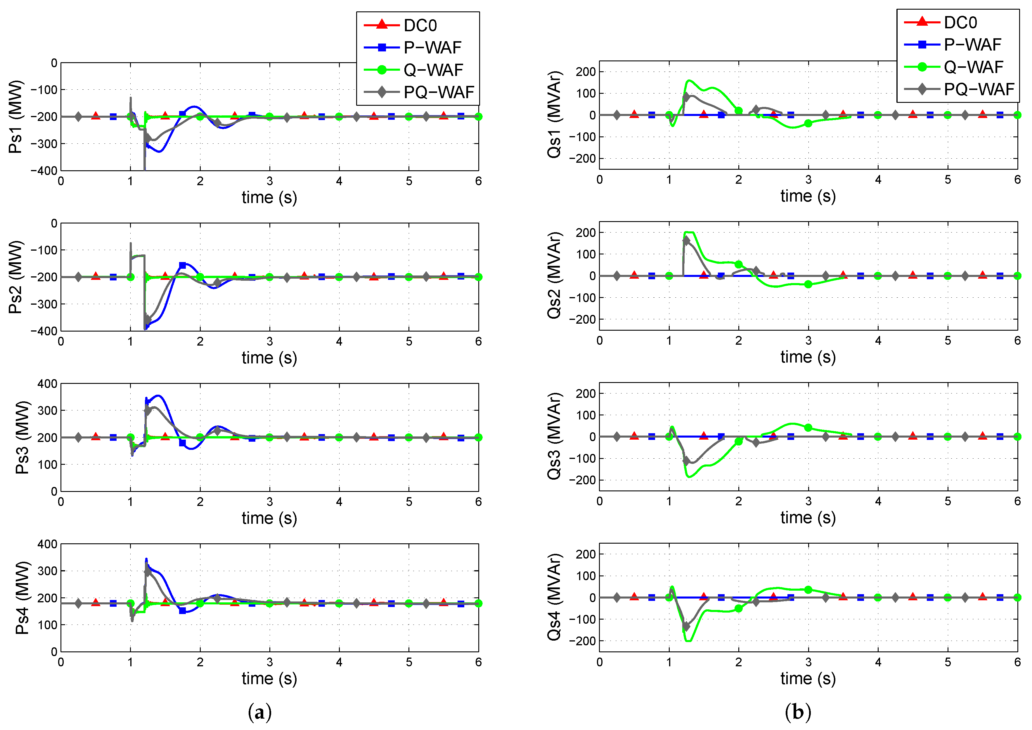
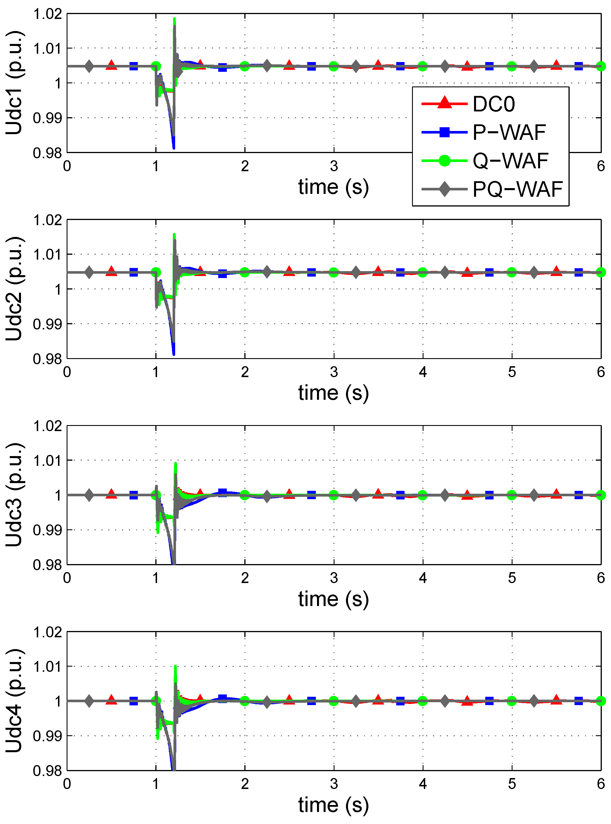
Figure 10 shows active- and reactive-power injections of the VSC stations into the AC grid, respectively. Without supplementary control (DC0), P and Q injections remain constant. In strategy P-WAF, P injections are modulated during the transient: immediately after the fault clearance, VSCs 1 and 2 reduce their P injections, since the frequencies measured by those converters are above the WAF. On the contrary, VSCs 3 and 4 increase their P injections, since their frequencies are below the WAF. In strategy Q-WAF, VSCs 1 and 2 increase their Q injections immediately after the fault clearance, while VSCs 3 and 4 reduce their Q injections. In strategy PQ-WAF, both, P and Q injections, are modulated simultaneously and this is why control effort is lower than the one in P-WAF and Q-WAF. By modulating P and Q injections of the VSC stations with strategies P-WAF, Q-WAF and PQ-WAF, the angles of generators are pulled together and transient stability is improved. Finally, Figure 11 shows the DC voltages of the converter stations, which remain close to 1 p.u. during the simulation.

4.1.2. Critical Clearing Times

The critical clearing time (CCT) is defined as the maximum time that a fault can remain before been cleared, without producing loss of synchronism and it is normally used as an indicator of a transient stability margin. The CCTs of the faults described in Table 1 are compared in Table 2, concluding that control strategies P-WAF, Q-WAF and PQ-WAF increase the CCTs significantly, with respect to the base case (DC0).

4.2. Impact of Communication Latency

The effect of latency on the frequencies measured by each VSC station to calculate the WAF in Equation (5) has been investigated. Each converter i will have a delay τ i i = 0 (zero delay applied to its own frequency measurement) and τ i j 0 (non-zero delay applied to the frequency measurements of the rest of VSC stations), when calculating the WAF.

4.2.1. Strategy P-WAF

The same fault as in Section 4.1.1 was simulated (Fault I of Table 1 cleared after 200 ms). Strategy P-WAF was implemented and the frequency signals were used by each converter to calculate the actual WAF communication latency. The following cases will be compared:
  • Strategy P-WAF, without communication latency ( τ i j = 0 ms).
  • Strategy P-WAF, with a communication latency of 50 ms ( τ i i = 0 ms and τ i j = 50 ms if i j ).
  • Strategy P-WAF, with a communication latency of 100 ms ( τ i i = 0 ms and τ i j = 100 ms if i j ).
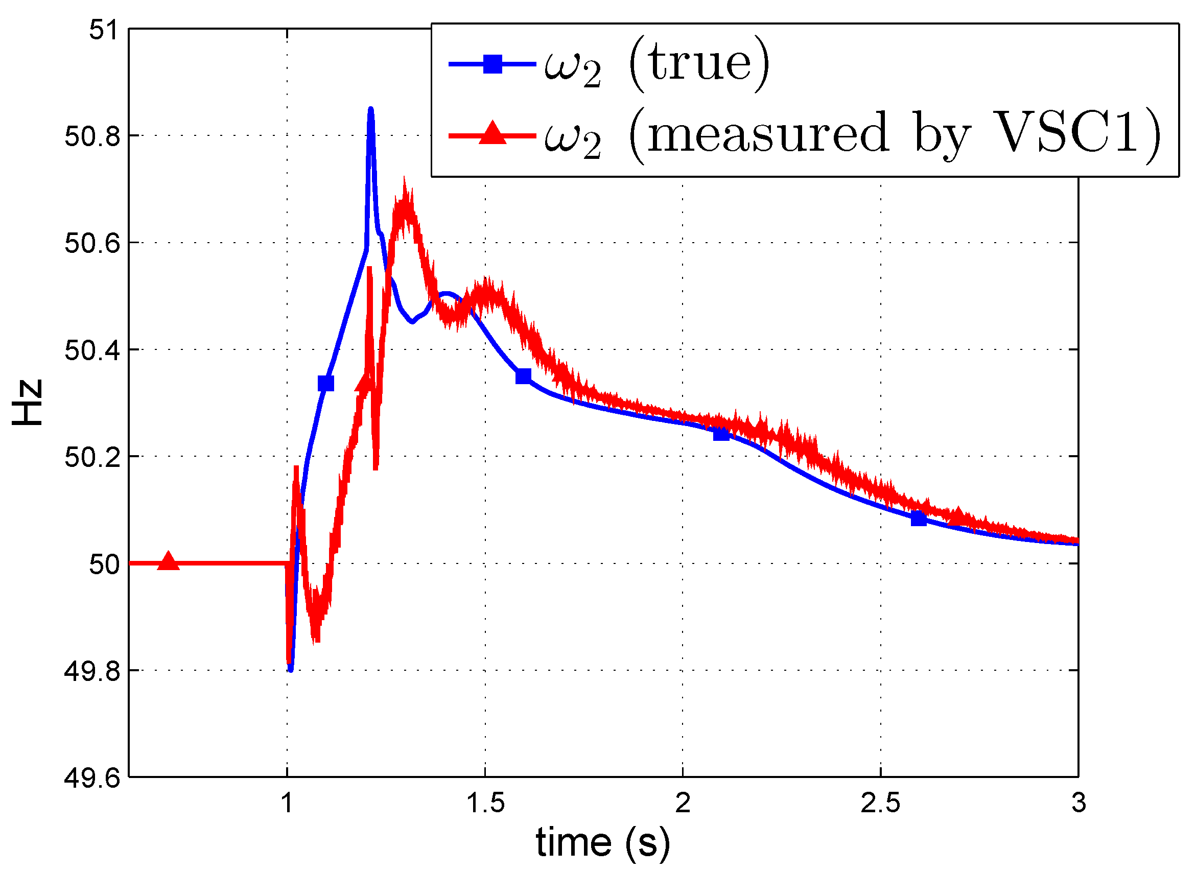
First of all, the impact of the communication delay on frequency measurements is illustrated: Figure 12 shows the true frequency at the AC terminal of VSC2 and the frequency of VSC2 measured by VSC1 when calculating the WAF, with a communication delay of τ 12 = 100 ms. Clearly, VSC1 sees the frequency of VSC2 delayed.
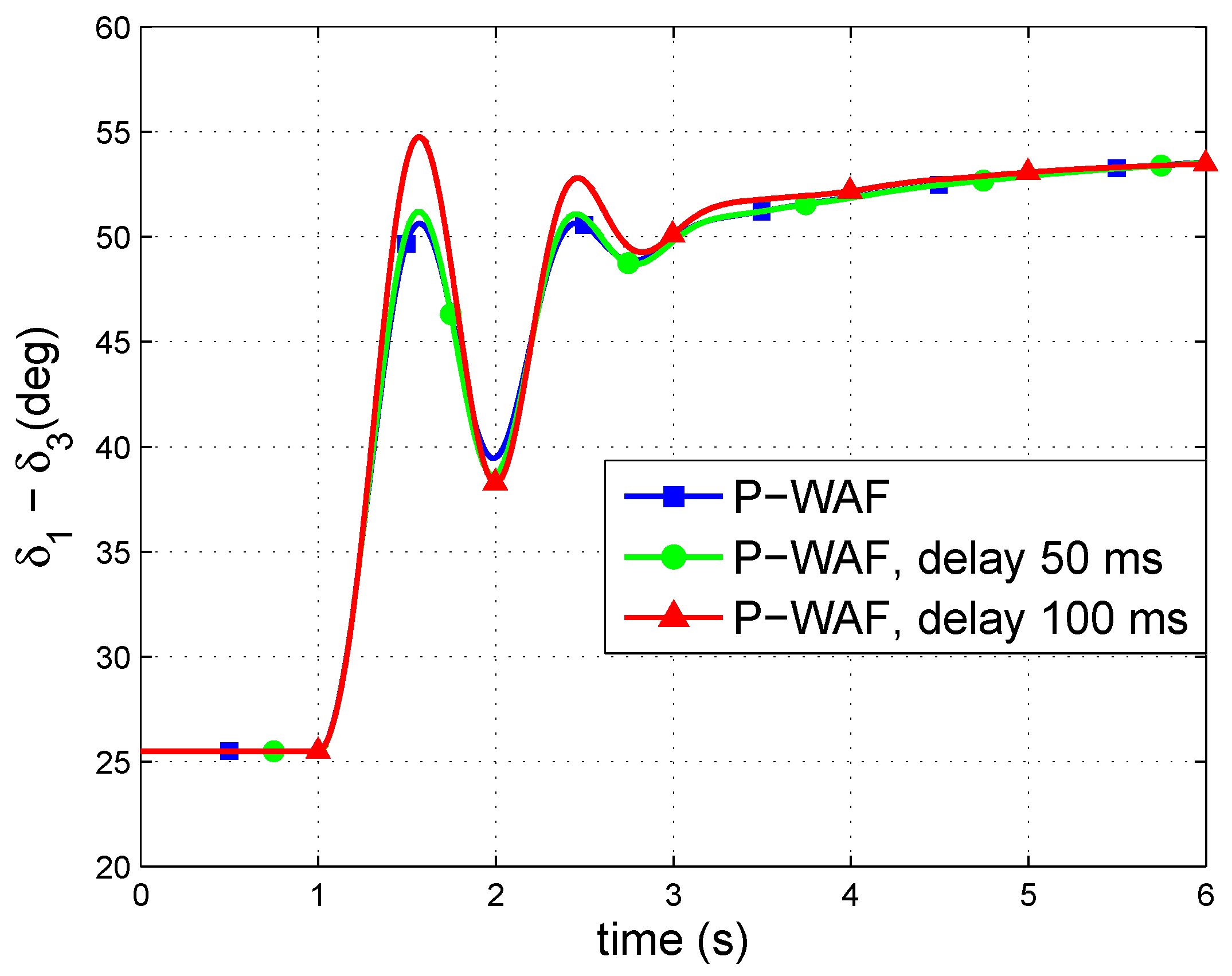
Results obtained with strategy P-WAF, with zero delay, τ i j = 50 ms and τ i j = 100 ms are shown in Figure 13 and Figure 14, respectively. The larger the communication delay is, the larger the generator-angle difference during the first swing is. However, the impact of communication latency on control strategy P-WAF is remarkable small and similar results are obtained in comparison to the case without communication latency. Notice that the time response of the P injections are very similar in the three cases (Figure 14a). This is due to the fact that strategy P-WAF and the DC-voltage droop are implemented together in all converter stations. Communication latency produces j = 1 n Δ p j r e f 0 , provoking DC-voltage fluctuations during the fault and immediately after its clearence (Figure 14b). These DC-voltage fluctuations are compensated with power sharing among all VSC stations thanks to the beneficial effect of the DC-voltage droop control implemented.

4.2.2. Strategy Q-WAF

Fault I of Table 1, cleared after 200 ms, was simulated. The following cases are compared:
  • Strategy Q-WAF, without communication latency ( τ i j = 0 ms).
  • Strategy Q-WAF, with a communication latency of 50 ms ( τ i i = 0 ms and τ i j = 50 ms if i j ).
  • Strategy Q-WAF, with a communication latency of 100 ms ( τ i i = 0 ms and τ i j = 100 ms if i j ).
Figure 15 shows the generator-angle differences, while Figure 16 shows Q injections of the VSC stations. Q-WAF clearly deteriorates with communication latency. This effect is more noticeable than when using strategy P-WAF. However, synchronism is maintained in all three cases. Q modulation with communication latency differs from the one with τ i j = 0 ms (Figure 16). Notice that, in the presence of communication latency, Q injections of VSCs 1 and 2 reach their limits (200 MVAr) during the fault and immediately after the fault clearance (Figure 16). The plots of P injections and DC voltages are omitted, since reactive-power control is independent of power sharing and DC voltages of the VSC-MTDC system.

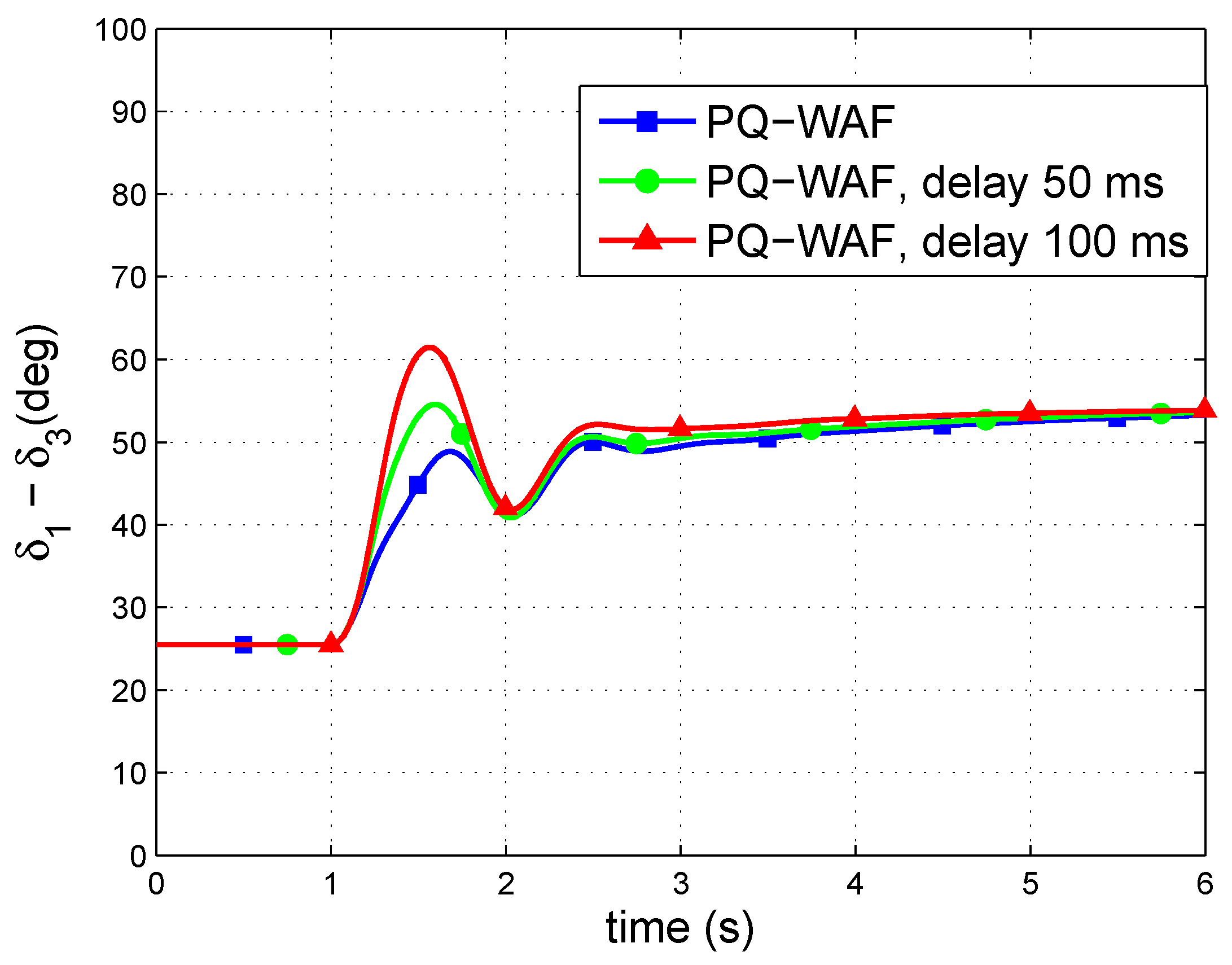
4.2.3. Strategy PQ-WAF

The effect of communication latency on strategy PQ-WAF was also analysed. Again, Fault I of Table 1, cleared after 200 ms, was simulated. The following cases are compared:
  • Strategy PQ-WAF, without communication latency ( τ i j = 0 ms).
  • Strategy PQ-WAF, with a communication latency of 50 ms ( τ i i = 0 ms and τ i j = 50 ms if i j ).
  • Strategy PQ-WAF, with a communication latency of 100 ms ( τ i i = 0 ms and τ i j = 100 ms if i j ).
Figure 17 shows the generator-angle differences. Results deteriorate with communication latency although stability is maintained in all three cases. The rest of the plots are omitted (P injections, Q injections and DC voltages), since they do not help understanding the system performance.

4.2.4. Critical Clearing Times

Table 3 shows the CCTs for the faults of Table 1, obtained with strategies P-WAF, Q-WAF and PQ-WAF, with communication latency of 50 ms and 100 ms. This case is called Case A, for further comparison with other cases in Section 4.3. The CCTs of all faults decrease as the communication latency increases, for all the control strategies. As already discussed, the impact of communication latency is more noticeable in strategy Q-WAF (Q injections) than in strategy P-WAF (P injections). The CCTs for all faults, obtained with the three control strategies and with a communication latency of 100 ms, are significantly higher than those obtained in the base case (DC0).
Finally, Figure 18 shows the CCT for Fault I versus communication-latency delay ( τ i j ) (from 0 ms to 250 ms, using a step of 50 ms). The CCT of the base case (DC0) is included in Figure 18 for comparison purposes. An indicator η is also plotted in Figure 18, which is defined as the CCT obtained with a certain control strategy divided by the CCT obtained in the base case:
η = C C T ( control   strategy ) C C T ( D C 0 )
As τ i j increases, the CCTs obtained with strategies Q-WAF and PQ-WAF decrease faster that the CCT obtained with strategy P-WAF (Figure 18). Notice that, in all three strategies, the CCTs obtained with τ i j = 250 ms are greater than the CCT obtained in the base case (DC0). Therefore, strategies P-WAF, Q-WAF and PQ-WAF proved to be robust against communication latency (see the percentage values of η in Figure 18).

4.3. Further Analysis of the Impact of Communication Latency: Equal versus Different Delays in the Communication Channels

A communication system between the VSC stations can be implemented in several ways. For example, frequency measurements at the AC side of all VSC stations can be collected by a central controller in order to be later distributed so that each converter can calculate the WAF according to Equation (5). Alternatively, each VSC station could be communicated directly with the others. Different communication arrangements will produce different latency patterns. There are two key aspects of communication latency that could affect the performance of the control strategies:
  • Total communication delay for frequency measurements at the VSC stations: having a delayed WAF instead of its true value.
  • Different communication delays for frequency measurements at the VSC stations: having a perturbed WAF instead of its true value, caused by different values of the communication delays of each frequency measurement.
The robustness of control strategies P-WAF, Q-WAF and PQ-WAF has been analysed in the following three cases:
  • Case A: Equal delay for all frequency measurements: τ i j = 50 ms, 100 ms, if i j , except for the frequency measured at the VSC station that calculates the WAF, that has zero delay ( τ i i = 0 ms) (this is the case analysed in Section 4.2). This case represents a communication system where frequency measurements at the VSC-MTDC systems are collected by a central controller and sent to each VSC station. Each VSC station uses those measurements to calculate the WAF.
  • Case B: Equal delay for all frequency measurements: τ i j = 50 ms, 100 ms, i , j . This case represents a communication system where frequency measurements at the VSC-MTDC systems are collected by a central controller and the central controller calculates the WAF, which is send, later, to all VSC stations.
  • Case C: Different delays for frequency measurements: τ i j , i , j , is obtained as a random number in the range [ 0 , Δ τ ] , following a uniform distribution ( τ i j U ( 0 , Δ τ ) ). The values of the delays are maintained constant during the simulation. Two values of Δ τ are used: 50 ms and 100 ms. Samples obtained for τ i j are given in Table 4. This case represents a communication system with communication channels between all the VSC stations.
  • Case D: Stochastic delays for frequency measurements: At each time step, the delay τ i j , if   i j , is obtained as a random number following a triangular distribution with mean τ i j 0 and upper/lower limits τ i j 0 ± Δ τ i j . The probability density function of the triangular distribution of τ i j is shown in Figure 19. Hence, the delay will be within the range:
    τ i j = τ i j 0 ± Δ τ i j
    As in case A, the frequency measured at the VSC station that calculates the WAF will have a zero delay ( τ i i = 0 ms). Two delays will be tested: τ i j = 50 ± 10 ms and τ i j = 100 ± 20 ms. Stochastic delays introduce noise, as shown in Figure 20. This case represents a more realistic version of Case A.
CCTs for the faults of Table 1 obtained in cases A, B, C and D are reported in Table 3 of Section 4.2 and Table 5, Table 6 and Table 7 respectively. In the four cases, CCTs decrease as the communication latency increases and, again, communication latency have a greater impact on strategy Q-WAF than on strategy P-WAF. Nevertheless, even in the presence of communication latency CCTs obtained with the control strategies outperform those obtained in the base case (DC0). Furthermore, no significant differences are observed in cases A (equal delay for all frequency measurements except for the frequency of the VSC station that calculates the WAF, that has τ i i = 0 ms), B (equal delay for all frequency measurements), C (different delays for frequency measurements) and D (stochastic delays for frequency measurements). Moreover, notice that the results of case A (Table 3 of Section 4.2) and case D (Table 7) are practically the same. This proves that the control strategies are robust against noisy delays and this is due to the low-pass filter used in the control schemes ( 1 / ( 1 + T f s ) in Figure 4 and Figure 5).

4.4. Further Research on the Impact of Communication Latency on Strategy P-WAF with Centralised DC-Voltage Control

So far, strategy P-WAF has been implemented in all VSC stations together with DC-voltage droop control (distributed DC-voltage control). As proved in Section 4.2.1, the presence of the latter mitigated the impact of communication latency. This Section investigated the case in which a DC-slack converter controls its DC voltage (centralised DC-voltage control) and all other converters control their P injections according to strategy P-WAF, only (there is not DC-voltage droop control). When modulating P injections in a VSC-MTDC system with centralised DC-voltage control, overloading of the DC-slack converter should be avoided.
Tests reported in this Section have been carried out within the following scenario:
  • VSC4 controled its DC voltage to 1 p.u (DC slack).
  • VSCs 1, 2 and 3 controled their P injections, using strategy P-WAF. Saturation parameters of the supplementary controller were set to Δ p i m a x = 0.2 p.u., in order to avoid overloading of the DC slack converter.
  • VSC2 was given the role of DC-slack converter, with DC-voltage limits u d c , i m a x = 1.1 p.u. and u d c , i m i n = 0.9 p.u.
  • DC-voltage limits of VSCs 1 and 3 were set to u d c , i m a x = 1.25 p.u. and u d c , i m i n = 0.7 p.u., in order to avoid interactions in case that the DC slack is overloaded.
Fault I of Table 1, cleared after 200 ms, was simulated and the following cases were compared:
  • Strategy P-WAF (with VSC4 as DC slack), without communication latency ( τ i j = 0 ms).
  • Strategy P-WAF (with VSC4 as DC slack), with a communication latency of 50 ms ( τ i i = 0 ms and τ i j = 50 ms if i j ).
  • Strategy P-WAF (with VSC4 as DC slack), with a communication latency of 100 ms ( τ i i = 0 ms and τ i j = 100 ms if i j ).
Figure 21 shows the generator-angle difference. Transient stability deteriorates with communication latency and the impact of the communication delay is more noticeable than when using strategy P-WAF together with DC-voltage droop control. Nevertheless, synchronism is maintained in all cases. Figure 22 shows P injections of the VSC stations and DC voltages. VSC stations 1, 2 and 3 modulate their P injections, while VSC4 controls its DC voltage to 1 p.u. Voltages at all DC buses are close to 1 p.u. during the whole simulation.
The CCTs for the faults of Table 1 are shown in 
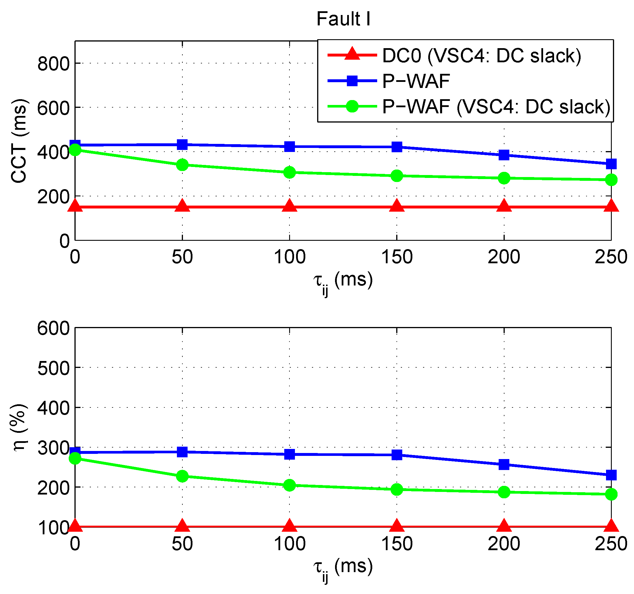
Table 8. As the communication delays increase, the CCTs decrease. Regardless of the communication latency, CCTs are significantly higher than those obtained in the base case (DC0, with VSC4 as DC slack). Finally, Figure 23 shows the CCT and indicator η of Fault I as a function of communication latency. The same scale of Figure 18 is used, to facilitate the comparison of the results. The CCT obtained with strategy P-WAF (and DC-voltage droop) is also plotted. In this case, the CCT of Fault I decreases as the communication delay increases, faster than in the case of P-WAF together with the DC-voltage frequency droop. The CCT obatined for τ i j = 250 ms is much higher than the one obtained in the base case.
Results show that strategy P-WAF, when implemented in a VSC-MTDC with centralised DC-voltage control (a single DC slack converter), is robust against communication latency although better results are obtained when implementing strategy P-WAF together with DC-voltage droop control.

5. Case Study 2: Cigré Nordic32A Test System with an Embedded VSC-MTDC System

The Cigré Nordic32A test system [55] with an embedded 3-terminal VSC-MTDC system was used for simulation (Figure 24). The objective of using this system is to test the control strategy in a larger multi-machine system, in order to test the scalability of the conclusions. Data are detailed in Appendix B. Converter stations were operated with DC-voltage droop control and reactive-power control. Simulations were carried out in PSS/E software [46], with the VSC-MTDC model presented in [44].
The initial operating point of the VSC-MTDC system was calculated running an AC/DC power flow, with the following specified variables:
  • VSC1: P s , 1 0 = 350 MW and Q s , 1 0 = 0 MVAr.
  • VSC2: P s , 2 0 = 500 MW and Q s , 2 0 = 150 MVAr.
  • VSC3: u d c , 3 0 = 1 p.u and Q s , 3 0 = 100 MVAr (VSC3 is used as the DC-slack converter for power-flow calculation).
The following cases have been analysed and compared:
  • DC0: No supplementary control strategy in the VSC stations.
  • Strategy P-WAF (P injections of VSC stations).
  • Strategy Q-WAF (Q injections of VSC stations).
  • Strategy PQ-WAF (simultaneous modulation of P and Q injections of VSC stations).
Since a detailed analysis has been presented in Section 4, this section will focus on the main results, only. The CCTs of the faults described in Table 9 have been calculated. Fault I is the most severe one, since corridor 4031–4041 carries a large amount of power in the operating point considered and both circuits of the corridor are disconnected after the fault clearing.
The performance of control strategies P-WAF, Q-WAF and PQ-WAF has been tested in the following three cases:
  • Case A: Equal delay for all frequency measurements: τ i j = 50 ms , 100 ms , if i j , except for the frequency measured at the VSC station that calculates the WAF, that has zero delay ( τ i i = 0 ms).
  • Case B: Equal delay for all frequency measurements: τ i j = 50 ms , 100 ms , i , j .
  • Case C: Different delays for frequency measurements: τ i j , i , j , is obtained as a random number in the range [ 0 , Δ τ ] , following a uniform distribution ( τ i j U ( 0 , Δ τ ) ). The values of the delays are maintained constant during the simulation. Two values of Δ τ are used: 50 ms and 100 ms. Samples obtained for τ i j are provided in Table 10.
  • Case D: Stochastic delays for frequency measurements: At each time step, the delay τ i j , if i j , is obtained as a random number following a triangular distribution with mean τ i j 0 and upper/lower limits τ i j 0 ± Δ τ i j . The probability density function of the triangular distribution of τ i j is shown in Figure 19. The frequency measured at the VSC station that calculates the WAF will have a zero delay ( τ i i = 0 ms). Two delays will be tested: τ i j = 50 ± 10 ms and τ i j = 100 ± 20 ms.
Table 11, Table 12, Table 13 and Table 14 report the CCTs obtained for the faults of Table 9, for cases A–D. Without communication latency, control strategies increase the CCTs significantly. For example, the CCT of Fault I increases from 105 ms in the base case DC0 to 390, 370 and 404 ms, with control strategies P-WAF, Q-WAF and PQ-WAF, respectively. The three control strategies proved to be robust against communication latency. Results with control strategies P-WAF and PQ-WAF are similar to those obtained without communication latency. As already discussed, communication latency have more impact when modulating reactive-power injections (Q-WAF). For example, with communication delays of 50 ms and 100 ms in case A (Table 11), the CCTs of Fault I are 317 ms and 160 ms, respectively. Those results still improve the base case (CCT of 105 ms), but below the improvement without communication latency (CCT of 370 ms). The CCTs of cases A–D (Table 11, Table 12, Table 13 and Table 14) follow a similar pattern and there are no signicant differences regarding the impact of the different type of delays considered.
Faults III and IV are also interesting to discuss. Fault III is almost unaffected by the control strategies and its CCT cannot be improved. The impact of strategy Q-WAF on Fault IV has a surprising pattern, since its CCT increases as the communication latency increases (when using Q-WAF). This was already observed in [39].
Finally, Figure 25 shows the CCT and η of Fault I (the most severe and challenging fault) as a function of communication latency of Case A. Control strategies P-WAF and PQ-WAF present significant improvements, even for large communication delays. In fact, the CCTs obtained are very similar to those obtained without communication delays. The performance of strategy Q-WAF worsens much faster as the value of the communication delay increases. Furthermore, for communication delays of τ i j = 200 ms and τ i j = 250 ms, the performance of strategy Q-WAF is very poor and results are worse than in the base case (a CCT of 0 ms means that the tripping of lines 4031-4041a&b produces loss of synchronism, even if there is no solid short circuit). This implies that control strategy Q-WAF requires fast communication systems to be effective (delays should not be greater than 100 ms).

6. Conclusions

This paper analysed the impact of communication latency on transient-stability-tailored control strategies in VSC-MTDC systems based on the weighted-average frequency (WAF) calculated by the VSC stations. Conclusions can be summarised as follows:
  • Strategies P-WAF (modulation of P injections), Q-WAF (modulation of Q injections) and PQ-WAF (simultaneous modulation of P and Q injections), implemented at the VSC stations of MTDC systems, improve transient stability, significantly.
  • Strategies P-WAF, Q-WAF and PQ-WAF improve transient stability, significantly, even when subject to communication latency, for realistic values of communication delays.
  • Strategy Q-WAF is more sensitive to communication latency than control strategy P-WAF.
  • Strategies P-WAF, Q-WAF and PQ-WAF proved to be robust against different types of communication latency (the same communication delay for all frequency measurements and different communication delays for the frequency measurements).
  • Strategy P-WAF implemented in a VSC-MTDC system with a single DC-slack converter is more sensitive to communication latency than control strategy P-WAF implemented in a VSC-MTDC system where converters have DC-voltage droop control.

Author Contributions

J.R., A.G.-C., L.R. and L.S. decided to investigate in detail the impact of communication latency on the transient-stability-tailored control strategies in VSC-MTDC systems (main contribution of the paper). J.R. ran the simulations and wrote the first version of the manuscript. J.R., A.G.-C., L.R. and L.S. improved the manuscript and elaborated the conclusions of this study.

Funding

Work supported by the Spanish Government under Project ENE2014-57760-C2-1R of the Spanish RETOS programme and by Madrid Regional Government under PRICAM-CM Project, Ref. S2013/ICE-2933. Work continues supported by PROMINT-CM Ref. S2018/EMT-4366, funded by Madrid Regional Government.

Conflicts of Interest

The authors declare no conflict of interest.

Appendix A. Data of the Case Study 1: Kundur’s Two-Area Test System with an Embedded VSC-MTDC System

Appendix A.1. HVAC Grid

Data of the HVAC system can be found in [54]. In the original test system, the nominal voltage of the transmission system and the nominal frequency were 230 kV and 60 Hz, respectively and those values have been changed to 220 kV and 50 Hz, respectively, in this work.
Synchronous machines are represented with a 6th-order dynamic model, with parameters:
S N = 900 MVA , H = 4.5   s   ( G 1 , G 2 ) , H = 4.175   s   ( G 3 , G 4 ) , D = 0 , T d 0 = 8   s , T d 0 = 0.03   s , T q 0 = 0.4   s , T q 0 = 0.05   s , X d = 1.8   p . u , X q = 1.7   p . u , X d = 0.3   p . u , X q = 0.55   p . u , X d = X q = 0.25   p . u , X l = 0.2   p . u , S ( 1.0 ) = 0.0435   p . u , S ( 1.2 ) = 0.2963   p . u .
Generators are equipped with a bus-fed static excitation system, as shown in Figure A1, with parameters:
T R = 0.01   s , K A = 200   p . u , K C = 0   p . u , E E M A X = 6.4   p . u , E E M I N = 6.4   p . u , E F D m a x = 6.4   p . u , E F D m i n = 6.4   p . u .
The generators are also equipped with a power system stabiliser (PSS) (STAB1 PSS/E library model [56]), with parameters:
K / T = 20   s 1 , T = 10   s , T 1 / T 3 = 2.5 , T 3 = 0.02   s , T 2 / T 4 = 0.5555 , T 4 = 5.4   s , H L I M = 0.05   p . u .
The governor system of the generators use IEEEG1 PSS/E library models [56], with parameters:
K = 20   p . u , T 1 = T 2 = 0   s , T 3 = 0.3   s , U o = 1   p . u . / s , , U c = 1   p . u . / s , P M A X = 1   p . u , P M I N = 0   p . u , T 4 = 0.3   s , K 1 = 0.3   p . u , K 2 = 0   p . u , T 5 = 7   s , K 3 = 0.3   p . u , K 4 = 0   p . u , T 6 = 0.6   s , K 5 = K 6 = K 7 = K 8 = 0   p . u , T 7 = 0   s .
For time-domain simulation, loads are represented with constant active current and with constant impedance for the reactive-power part.
The following modifications were made in order to consider a critical case for transient stability:
  • Inertia constants: H 1 = H 2 = 4.5 s and H 3 = H 4 = 4.175 s.
  • Loads: 467 MW and 100 MVAr at bus 7 and 2267 MW and 0 MVAr at bus 9.
Figure A1. Excitation system.
Energies 12 03638 g0a1

Appendix A.2. VSC-MTDC System

Table A1. Converter and HVDC grid parameters.
Parameters
VSC’s Rating are Base Values for p.u.
Rating VSC, DC voltage, AC voltage500 MVA, ± 320 kV, 300 kV
ConfigurationSymmetrical monopole
Max. active (reactive) power ± 500 MW ( ± 200 MVAr)
Max. current1 p.u (d-axis priority)
Max. DC voltage ± 10 %
Max. modulation index1.31 p.u
Current-controller time constant ( τ )5 ms
Connection resistance ( r s )/reactance ( x s )0.02 p.u / 0.20 p.u
(reactor + 300/220 kV transformer)
P prop./int. control: ( K d , p 1 / K d , i 1 )0/0 (i.e. i d , i r e f = p s , i r e f / u s , i )
Vdc prop./int. control ( K d , p 2 / K d , i 2 )4 p.u/0.24 p.u/s
Q-control prop./int. control: ( K q , p 1 / K q , i 1 )0/0 (i.e. i q , i r e f = q s , i r e f / u s , i )
DC-voltage droop constant ( k d c , i )0.1 p.u
VSCs’ loss coefficients (a/b) in p.u.5.25/1.65 × 10 3 p.u.
VSCs’ loss coefficients ( c r e c / c i n v ) in p.u.2.10/3.14 × 10 3 p.u.
DC-bus capacitance ( C d c , i )195 μ F
DC-line series parameters ( R d c , i j / L d c , i j )0.51 Ω /35.03 mH (lines 1–2 & 3–4)
5.23 Ω /357.26 mH (line 1–3)
4.92 Ω /336.24 mH (line 2–4)

Appendix A.3. Parameters of the Control Strategies

  • Strategy P-WAF: Block diagram of Figure 4, with parameters: k P , i = 200 p.u, T f , i = 0.1 s, T W , i = 15 s, Δ p m a x , i = 0.4 p.u and α k = 1 / 4 . The gains are in nominal p.u. The frequency set point is calculated as Equation (5).
  • Strategy Q-WAF: Block diagram of Figure 5, with parameters: k Q , i = 200 p.u, T f , i = 0.1 s, T W , i = 15 s, Δ q m a x , i = 0.4 p.u and α k = 1 / 4 . The gains are in nominal p.u. The frequency set point is calculated as Equation (5).
  • Strategy PQ-WAF: Strategies P-WAF and Q-WAF are implemented simultaneously. The same parameters of strategies P-WAF and Q-WAF are used.

Appendix B. Data of the Case Study 2: Cigré Nordic32A Test System with an Embedded VSC-MTDC System

Appendix B.1. HVAC Grid

Data of the HVAC system can be found in [55,57]. A comprehensive description of the system, with the analysis of different operating points, can be found in [58]. A heavily loaded operating point is considered in this work, with the modifications of Table A2. Loads are modelled with a constant impedance characteristic for dynamic simulation.
Table A2. Modifications of Nordic32A case.
Original ValueNew Value
LoadsBus 1044800 MW1300 MW
Bus 41540 MW620 MW
Bus 4071 (equiv.)300 MW0 MW
Bus 4072 (equiv.)2000 MW1840 MW
Bus 62300 MW200 MW
ShuntsBuses 1044 and 4041200 MVAr300 MVAr

Appendix B.2. VSC-MTDC System

Table A3. Converter and HVDC grid parameters.
Parameters
VSC’s Rating are Base Values for p.u.
Rating VSC, DC voltage, AC voltage1000 MVA, ± 320 kV, 300 kV
ConfigurationSymmetrical monopole
Max. active (reactive) power ± 1000 MW ( ± 450 MVAr)
Max. current1 p.u (d-axis priority)
Max. DC voltage ± 10 %
Max. modulation index1.31 p.u
Current-controller time constant ( τ )5 ms
Connection resistance ( r s )/reactance ( x s )0.002 p.u / 0.17 p.u
(reactor + 300/400 kV transformer)
P prop./int. control: ( K d , p 1 / K d , i 1 )0/0 (i.e., i d , i r e f = p s , i r e f / u s , i )
Vdc prop./int. control ( K d , p 2 / K d , i 2 )2 p.u/0.12 p.u/s
Q-control prop./int. control: ( K q , p 1 / K q , i 1 )0/0 (i.e., i q , i r e f = q s , i r e f / u s , i )
DC-voltage droop constant ( k d c , i )0.1 p.u
VSCs’ loss coefficients (a/b) in p.u.11.033/3.464 × 10 3 p.u.
VSCs’ loss coefficients ( c r e c / c i n v ) in p.u.4.40/6.67 × 10 3 p.u.
DC-bus capacitance ( C d c , i )195 μ F
DC-line series parameters ( R d c , i j / L d c , i j )2.05 Ω /140.10 mH

Appendix B.3. Parameters of the Control Strategies

  • Strategy P-WAF: Block diagram of Figure 4, with parameters: k P , i = 200 p.u, T f , i = 0.1 s, T W , i = 15 s, Δ p m a x , i = 1.0 p.u and α k = 1 / 3 . The gains are in nominal p.u. The frequency set point is calculated as Equation (5).
  • Strategy Q-WAF: Block diagram of Figure 5, with parameters: k Q , i = 200 p.u, T f , i = 0.1 s, T W , i = 15 s, Δ q m a x , i = 1.0 p.u and α k = 1 / 3 . The gains are in nominal p.u. The frequency set point is calculated as Equation (5).
  • Strategy PQ-WAF: Strategies P-WAF and Q-WAF are implemented simultaneously. The same parameters of strategies P-WAF and Q-WAF are used.

References

  1. Flourentzou, N.; Agelidis, V.G.; Demetriades, G.D. VSC-Based HVDC Power Transmission Systems: An Overview. IEEE Trans. Power Electron. 2009, 24, 592–602. [Google Scholar] [CrossRef]
  2. Gordon, S. Supergrid to the rescue. Power Eng. 2006, 20, 30–33. [Google Scholar] [CrossRef]
  3. Blau, J. Europe plans a North Sea grid. IEEE Spectr. 2010, 47, 12–13. [Google Scholar] [CrossRef]
  4. Van Hertem, D.; Ghandhari, M. Multi-terminal VSC HVDC for the European supergrid: Obstacles. Renew. Sustain. Energy Rev. 2010, 14, 3156–3163. [Google Scholar] [CrossRef]
  5. Bompard, E.; Fulli, G.; Ardelean, M.; Masera, M. It’s a Bird, It’s a Plane, It’s a... Supergrid. IEEE Power Energy Mag. 2014, 12, 41–50. [Google Scholar]
  6. Lesnicar, A.; Marquardt, R. An Innovative Modular Multilevel Converter Topology Suitable for a Wide Power Range. In Proceedings of the IEEE/PES PowerTech Conference, Bologna, Italy, 23–26 June 2003; pp. 1–6. [Google Scholar]
  7. Kouro, S.; Malinowski, M.; Gopakumar, K.; Pou, J.; Franquelo, L.G.; Wu, B.; Rodriguez, J.; Pérez, M.A.; Leon, J.I. Recent Advances and Industrial Applications of Multilevel Converters. IEEE Trans. Ind. Electron. 2010, 57, 2553–2580. [Google Scholar] [CrossRef]
  8. Bola, J.; Rivas, R.; Fernández-Alonso, R.; Pérez, G.; Hidalgo, J.; Coronado, L.M.; Longás, C.; Sanz, S.; Lemarchand, G.; Roguin, J.; et al. Operational experience of new Spain-France HVDC interconnection. In Proceedings of the CIGRE Session, Paper B4–117, Paris, France, 21 August 2016; pp. 1–13. [Google Scholar]
  9. Vrana, T.K.; Beerten, J.; Belmans, R.; Fosso, O.B. A classification of DC node voltage control methods for HVDC grids. Electr. Power Syst. Res. 2013, 103, 137–144. [Google Scholar] [CrossRef] [Green Version]
  10. Bianchi, F.D.; Domínguez-García, J.L.; Gomis-Bellmunt, O. Control of multi-terminal HVDC networks towards wind power integration: A review. Renew. Sustain. Energy Rev. 2016, 55, 1055–1068. [Google Scholar] [CrossRef] [Green Version]
  11. Prieto-Araujo, E.; Bianchi, F.D.; Junyent-Ferré, A.; Gomis-Bellmunt, O. Methodology for Droop Control Dynamic Analysis of Multiterminal VSC-HVDC Grids for Offshore Wind Farms. IEEE Trans. Power Deliv. 2011, 26, 2476–2485. [Google Scholar] [CrossRef]
  12. Egea-Alvarez, A.; Bianchi, F.; Junyent-Ferré, A.; Gross, G.; Gomis-Bellmunt, O. Voltage Control of Multiterminal VSC-HVDC Transmission Systems for Offshore Wind Power Plants: Design and Implementation in a Scaled Platform. IEEE Trans. Ind. Electron. 2013, 60, 2381–2391. [Google Scholar] [CrossRef]
  13. Berggren, B.; Lindén, K.; Majumder, R. DC Grid Control Through the Pilot Voltage Droop Concept—Methodology for Establishing Droop Constants. IEEE Trans. Power Syst. 2014, 30, 2312–2320. [Google Scholar] [CrossRef]
  14. Kirakosyan, A.; El-Saadany, E.F.; El Moursi, M.S.; Acharya, S.; Al Hosani, K. Control Approach for the Multi-Terminal HVDC System for the Accurate Power Sharing. IEEE Trans. Power Syst. 2018, 33, 4323–4334. [Google Scholar] [CrossRef]
  15. Häfner, J.; Jacobson, B. Device and Method to Break the Current of a Power Transmission or Distribution Line and Current Limiting Arrangement. European Patent EP2502248B1, 2009. [Google Scholar]
  16. Davidson, C.C.; Whitehouse, R.S.; Barker, C.D.; Dupraz, J.-P.; Grieshaber, W. A new ultra-fast HVDC Circuit breaker for meshed DC networks. In Proceedings of the 11th IET International Conference on AC and DC Power Transmission, Birmingham, UK, 10–12 February 2015; pp. 1–7. [Google Scholar]
  17. De Kerf, K.; Srivastava, K.; Reza, M.; Bekaert, D.; Cole, S.; Van Hertem, D.; Belmans, R. Wavelet-based protection strategy for DC faults in multi-terminal VSC HVDC systems. IET Gener. Transm. Distrib. 2011, 5, 496–503. [Google Scholar] [CrossRef]
  18. Descloux, J.; Rault, P.; Nguefeu, S.; Curis, J.B.; Guillaud, X.; Colas, P.; Raison, B. HVDC meshed grid: Control and protection of a multi-terminal HVDC system. In Proceedings of the CIGRE Session, Paris, France, 26–31 August 2012; pp. 1–8. [Google Scholar]
  19. Adamczyk, A.; Barker, C.D.; Ha, H. Fault Detection and Branch Identification for HVDC Grids. In Proceedings of the 12th IET International Conference on Developments in Power System Protection (DPSP), Copenhagen, Denmark, 31 March–3 April 2014; pp. 1–6. [Google Scholar]
  20. Leterme, W.; Beerten, J.; Van Hertem, D. Non-unit Protection of HVDC Grids With Inductive DC Cable Termination. IEEE Trans. Power Deliv. 2016, 31, 820–828. [Google Scholar] [CrossRef]
  21. Sneath, J.; Rajapakse, A.D. Fault Detection and Interruption in an Earthed HVDC Grid Using ROCOV and Hybrid DC Breakers. IEEE Trans. Power Deliv. 2016, 31, 973–981. [Google Scholar] [CrossRef]
  22. Torres-Olguin, R.E.; Hϕidalen, H.K. Travelling waves-based fault detection method in multi-terminal HVDC grids connecting offshore wind farms. In Proceedings of the 13th IET International Conference on Developments in Power System Protection (DPSP), Edinburgh, UK, 7–10 March 2016; pp. 1–7. [Google Scholar]
  23. Azad, S.P.; Van Hertem, D. A Fast Local Bus Current-Based Primary Relaying Algorithm for HVDC Grids. IEEE Trans. Power Deliv. 2017, 32, 193–202. [Google Scholar] [CrossRef]
  24. Tzelepis, D.; Dyśko, A.; Fusiek, G.; Nelson, J.; Niewczas, P.; Vozikis, D.; Orr, P.; Gordon, N.; Booth, C. Single-Ended Differential Protection in MTDC Networks using Optical Sensors. IEEE Trans. Power Deliv. 2017, 32, 1605–1615. [Google Scholar] [CrossRef]
  25. Yang, Q.; Le Blond, S.; Aggarwal, R.; Wang, Y.; Li, J. New ANN method for multi-terminal HVDC protection relaying. Electr. Power Syst. Res. 2017, 148, 192–201. [Google Scholar] [CrossRef] [Green Version]
  26. Latorre, H.; Ghandhari, M.; Söder, L. Active and reactive power control of a VSC-HVdc. Electr. Power Syst. Res. 2008, 78, 1756–1763. [Google Scholar] [CrossRef]
  27. Fuchs, A.; Imhof, M.; Demiray, T.; Morari, M. Stabilization of Large Power Systems Using VSC–HVDC and Model Predictive Control. IEEE Trans. Power Deliv. 2014, 29, 480–488. [Google Scholar] [CrossRef]
  28. Sigrist, L.; Echavarren, F.; Rouco, L.; Panciatici, P. A fundamental study on the impact of HVDC lines on transient stability of power systems. In Proceedings of the IEEE/PES PowerTech Conference, Eindhoven, The Netherlands, 29 June–2 July 2015; pp. 1–6. [Google Scholar]
  29. Martínez Sanz, I.; Chaudhuri, B.; Strbac, G. Coordinated Corrective Control for Transient Stability Enhancement in Future Great Britain Transmission System. In Proceedings of the 19th Power Systems Computation Conference (PSCC), Genoa, Italy, 24–26 June 2016; pp. 1–7. [Google Scholar]
  30. Kundur, P.; Paserba, J.; Ajjarapu, V.; Andersson, G.; Bose, A.; Canizares, C.; Hatziargyriou, N.; Hill, D.; Stankovic, A.; Taylor, C.; et al. Definition and classification of power system stability IEEE/CIGRE joint task force on stability terms and definitions. IEEE Trans. Power Syst. 2004, 19, 1387–1401. [Google Scholar]
  31. Zhou, Y.; Huang, H.; Xu, Z.; Hua, W.; Yang, F.; Liu, S. Wide-area measurement system-based transient excitation boosting control to improve power system transient stability. IET Gener. Transm. Distrib. 2015, 9, 845–854. [Google Scholar] [CrossRef]
  32. Díez-Maroto, L.; Vanfretti, L.; Almas, M.S.; Jónsdóttir, G.M.; Rouco, L. A WACS exploiting generator Excitation Boosters for power system transient stability enhancement. Electr. Power Syst. Res. 2017, 148, 245–253. [Google Scholar] [CrossRef]
  33. Díez-Maroto, L.; Renedo, J.; Rouco, L.; Fernández-Bernal, F. Lyapunov Stability Based Wide Area Control Systems for Excitation Boosters in Synchronous Generators. IEEE Trans. Power Syst. 2019, 34, 194–204. [Google Scholar] [CrossRef]
  34. Machowski, J.; Kacejko, P.; Nogal, L.; Wancerz, M. Power system stability enhancement by WAMS-based supplementary control of multi-terminal HVDC networks. Control. Eng. Pract. 2013, 21, 583–592. [Google Scholar] [CrossRef]
  35. Eriksson, R. Coordinated Control of Multiterminal DC Grid Power Injections for Improved Rotor-Angle Stability Based on Lyapunov Theory. IEEE Trans. Power Deliv. 2014, 29, 1789–1797. [Google Scholar] [CrossRef]
  36. Tang, G.; Xu, Z.; Dong, H.; Xu, Q. Sliding Mode Robust Control Based Active-Power Modulation of Multi-Terminal HVDC Transmissions. IEEE Trans. Power Syst. 2016, 31, 1614–1623. [Google Scholar] [CrossRef]
  37. Fan, X.; Shu, J.; Zhang, B. Coordinated Control of DC Grid and Offshore Wind Farms to Improve Rotor-Angle Stability. IEEE Trans. Power Syst. 2018, 33, 4625–4633. [Google Scholar] [CrossRef]
  38. Renedo, J.; García-Cerrada, A.; Rouco, L. Active Power Control Strategies for Transient Stability Enhancement of AC/DC Grids With VSC-HVDC Multi-Terminal Systems. IEEE Trans. Power Syst. 2016, 31, 4595–4604. [Google Scholar] [CrossRef]
  39. Renedo, J.; García-Cerrada, A.; Rouco, L. Reactive-Power Coordination in VSC-HVDC Multi-Terminal Systems for Transient Stability Improvement. IEEE Trans. Power Syst. 2017, 32, 3758–3767. [Google Scholar] [CrossRef]
  40. Milano, F.; Ortega, A. Frequency divider. IEEE Trans. Power Syst. 2017, 32, 1493–1501. [Google Scholar]
  41. Milano, F. Rotor Speed-Free Estimation of the Frequency of the Center of Inertia. IEEE Trans. Power Syst. 2018, 33, 1153–1155. [Google Scholar] [CrossRef]
  42. Cole, S.; Beerten, J.; Belmans, R. Generalized Dynamic VSC MTDC Model for Power System Stability Studies. IEEE Trans. Power Syst. 2010, 25, 1655–1662. [Google Scholar] [CrossRef]
  43. Beerten, J.; Cole, S.; Belmans, R. Modeling of Multi-Terminal VSC HVDC Systems With Distributed DC Voltage Control. IEEE Trans. Power Syst. 2014, 29, 34–42. [Google Scholar] [CrossRef]
  44. Renedo, J.; García-Cerrada, A.; Rouco, L.; Sigrist, L.; Egido, I.; Sanz Verdugo, S. Development of a PSS/E tool for power-flow calculation and dynamic simulation of VSC-HVDC multi-terminal systems. In Proceedings of the 13th IET International Conference on AC and DC Power Transmission, Manchester, UK, 14–16 February 2017; pp. 1–6. [Google Scholar]
  45. Daelemans, G.; Srivastava, K.; Reza, M.; Cole, S.; Belmans, R. Minimization of steady-state losses in meshed networks using VSC HVDC. In Proceedings of the IEEE/PES General Meeting, Calgary, AB, Canada, 26–30 July 2009; pp. 1–5. [Google Scholar]
  46. Siemens-PTI. PSS/E 33.5 Users Manual; Siemens Power Technologies International: Schenectady, NY, USA, 2013. [Google Scholar]
  47. Chainho, P.J.D. General Modeling of Multi-Terminal VSC-HVDC Systems for Transient Stability Analysis. Master’s Thesis, Universidade Técnica de Lisboa, Lisbon, Portugal, 2012. [Google Scholar]
  48. Chainho, P.J.D.; van der Meer, A.A.; Gibescu, M.; Hendriks, R.L.; van der Meijden, M.A.M.M. General Modeling of Multi-Terminal VSC-HVDC Systems for Transient Stability Studies. In Proceedings of the 6th IEEE Young Researchers Symposium in Electrical Power Engineering, Delft, The Netherlands, 16–17 April 2012; pp. 1–6. [Google Scholar]
  49. Ndreko, M. Offshore Wind Power Connected to the Dutch Transmission System by VSC-HVDC Networks: Modeling and Stability Analysis. Master’s Thesis, Delft University of Technology, Delft, The Netherlands, 2012. [Google Scholar]
  50. Liu, S.; Xu, Z.; Hua, W.; Tang, G.; Xue, Y. Electromechanical Transient Modeling of Modular Multilevel Converter Based Multi-Terminal HVDC Systems. IEEE Trans. Power Syst. 2014, 29, 72–83. [Google Scholar] [CrossRef]
  51. Beerten, J.; Cole, S.; Belmans, R. Generalized Steady-State VSC MTDC Model for Sequential AC/DC Power Flow Algorithms. IEEE Trans. Power Syst. 2012, 27, 821–829. [Google Scholar] [CrossRef]
  52. Zhang, F.; Sun, Y.; Cheng, L.; Li, X.; Chow, J.H.; Zhao, W. Measurement and Modeling of Delays in Wide-Area Closed-Loop Control Systems. IEEE Trans. Power Syst. 2015, 30, 2426–2433. [Google Scholar] [CrossRef]
  53. Chompoobutrgool, Y.; Vanfretti, L. Analysis of time delay effects for wide-area damping control design using dominant path signals. In Proceedings of the IEEE/PES General Meeting, National Harbor, MD, USA, 27–31 July 2014; pp. 1–5. [Google Scholar]
  54. Kundur, P. Power System Stability and Control; McGraw-Hill Education: New York, NY, USA, 1994. [Google Scholar]
  55. Stubbe (Convenor), M. Long Term Dynamics Phase II; Technical Report, Cigré Task Force 38.02.08–TB 102; CIGRE: Paris, France, 1995. [Google Scholar]
  56. Siemens-PTI. PSS/E 33.5 Model Library; Siemens Power Technologies International: Schenectady, NY, USA, 2013. [Google Scholar]
  57. Karlsson, B. Comparison of PSSE & PowerFactory; Degree Project; Uppsala Universitet: Uppsala, Sweden, 2013; Available online: https://www.diva-portal.org/smash/get/diva2:658793/FULLTEXT01.pdf (accessed on 20 September 2019).
  58. Van Cutsem, T.; Papangelis, L. Description, Modeling and Simulation Results of a Test System for Voltage Stability Analysis; Technical Report; Université de Liège: Liège, Belgium, 2014. [Google Scholar]
Figure 1. Hybrid voltage source converters (VSC)-based AC/DC system.
Energies 12 03638 g001
Figure 2. Model of a VSC and the DC grid [42].
Energies 12 03638 g002
Figure 3. (a) P control and (b) Q control.
Energies 12 03638 g003
Figure 4. Control for the active-power injection of a VSC.
Energies 12 03638 g004
Figure 5. Control for the reactive-power injection of a VSC.
Energies 12 03638 g005
Figure 6. Calculation of the frequency set point of VSC j in the presence of communication latency.
Energies 12 03638 g006
Figure 7. Kundur’s 2-area system with an embedded VSC-MTDC.
Energies 12 03638 g007
Figure 8. Generator angle difference.
Energies 12 03638 g008
Figure 9. Frequencies measured at the converter stations ( ω i ) and WAF ( ω ¯ ) (when using P-WAF).
Energies 12 03638 g009
Figure 10. (a) P and (b) Q injections of the converters.
Energies 12 03638 g010
Figure 11. DC voltages.
Energies 12 03638 g011
Figure 12. Strategy P-WAF with τ i j = 100 ms. Frequency of VSC2 measured by VSC1.
Energies 12 03638 g012
Figure 13. Strategy P-WAF: Impact of communication latency. Generator angle difference.
Energies 12 03638 g013
Figure 14. (a) P injections of the converters and (b) DC voltages.
Energies 12 03638 g014
Figure 15. Generator angle difference.
Energies 12 03638 g015
Figure 16. Q injections of the converters.
Energies 12 03638 g016
Figure 17. Generator angle difference.
Energies 12 03638 g017
Figure 18. CCTs and η versus communication delay.
Energies 12 03638 g018
Figure 19. Case D: Communication delays follow a triangular distribution. Probability density function.
Energies 12 03638 g019
Figure 20. Case D. Strategy P-WAF with τ i j = 100 ± 20 ms (triangular distribution). Frequency of VSC2 measured by VSC1.
Energies 12 03638 g020
Figure 21. Generator angle difference.
Energies 12 03638 g021
Figure 22. (a) P injections of the converters and (b) DC voltages.
Energies 12 03638 g022
Figure 23. CCTs and η versus communication delay.
Energies 12 03638 g023
Figure 24. Cigré Nordic 32A system with an embedded VSC-MTDC system.
Energies 12 03638 g024
Figure 25. Case A. CCTs and η versus communication delay.
Energies 12 03638 g025
Table 1. Faults.
Table 1. Faults.
Short Circuit at Line i j Close to BusClearing
Fault I7–8 a7Disconnection of line 7–8 a
Fault II5–65Short circuit cleared (line not disconnected)
Fault III10–1110Short circuit cleared (line not disconnected)
Table 2. Critical clearing times (CCT).
CCTs (ms)Fault IFault IIFault III
DC0150178189
P-WAF430242479
Q-WAF726423339
PQ-WAF828369585
Table 3. Case A. CCT. Effect of communication latency.
CCTs (ms)Fault IFault IIFault III
DC0150178189
P-WAF430242479
P-WAF, delay 50 ms433242443
P-WAF, delay 100 ms436243381
Q-WAF726423339
Q-WAF, delay 50 ms428398295
Q-WAF, delay 100 ms273312287
PQ-WAF828369585
PQ-WAF, delay 50 ms566332534
PQ-WAF, delay 100 ms444291471
Table 4. Case C. Communication delays used ( τ i j (ms)).
τ ij (ms)VSC τ i 1 τ i 2 τ i 3 τ i 4
Δ τ = 50  msVSC1: τ 1 j 646325
VSC2: τ 2 j 14274848
VSC3: τ 3 j 8494824
VSC4: τ 4 j 4072146
Δ τ = 100  msVSC1: τ 1 j 7996664
VSC2: τ 2 j 85936876
VSC3: τ 3 j 74396617
VSC4: τ 4 j 713285
Table 5. Case B. CCT.
CCTs (ms)Fault IFault IIFault III
DC0150178189
P-WAF430242479
P-WAF, delay: τ i j = 50  ms i , j 432242429
P-WAF, delay: τ i j = 100  ms i , j 423242351
Q-WAF726423339
Q-WAF, delay: τ i j = 50  ms i , j 365376290
Q-WAF, delay: τ i j = 100  ms i , j 242273277
PQ-WAF828369585
PQ-WAF, delay: τ i j = 50  ms i , j 518324519
PQ-WAF, delay: τ i j = 100  ms i , j 397273440
Table 6. Case C. CCT.
CCTs (ms)Fault IFault IIFault III
DC0150178189
P-WAF430242479
P-WAF, delay: τ i j U ( 0 , 50  ms) i , j 427242459
P-WAF, delay: τ i j U ( 0 , 100  ms) i , j 412242414
Q-WAF726423339
Q-WAF, delay: τ i j U ( 0 , 50  ms) i , j 492412295
Q-WAF, delay: τ i j U ( 0 , 100  ms) i , j 421392291
PQ-WAF828369585
PQ-WAF, delay: τ i j U ( 0 , 50  ms) i , j 584345542
PQ-WAF, delay: τ i j U ( 0 , 100  ms) i , j 505320511
Table 7. Case D. CCT.
CCTs (ms)Fault IFault IIFault III
DC0150178189
P-WAF430242479
P-WAF, delay: τ i j = 50 ± 10  ms433242443
P-WAF, delay: τ i j = 100 ± 20  ms436243382
Q-WAF726423339
Q-WAF, delay: τ i j = 50 ± 10  ms429400295
Q-WAF, delay: τ i j = 100 ± 20  ms275312287
PQ-WAF828369585
PQ-WAF, delay: τ i j = 50 ± 10  ms566332534
PQ-WAF, delay: τ i j = 100 ± 20  ms444291471
Table 8. CCT. Effect of communication latency on strategy P-WAF when the VSC-MTDC system has a single DC slack.
CCTs (ms)Fault IFault IIFault III
DC0 (VSC4: DC slack)150200225
P-WAF (VSC4: DC slack)408273296
P-WAF (VSC4: DC slack), delay 50 ms341260303
P-WAF (VSC4: DC slack), delay 100 ms307253301
Table 9. Faults.
Table 9. Faults.
Short Circuit at Line i j Close to BusClearing
Fault I4031–4041a4041Disconnect 4031–4041 a&b
Fault II4012–40224012Line disconnected
Fault III4012–40224022Line disconnected
Fault IV4032–40444044Line disconnected
Fault V4011–40224011Line disconnected
Table 10. Case C. Communication delays used ( τ i j (ms)).
τ ij (ms)VSC τ i 1 τ i 2 τ i 3
Δ τ = 50  msVSC1: τ 1 j 2541
VSC2: τ 2 j 351641
VSC3: τ 3 j 22219
Δ τ = 100  msVSC1: τ 1 j 778019
VSC2: τ 2 j 494565
VSC3: τ 3 j 717528
Table 11. Case A. CCT. Effect of communication latency.
CCTs (ms)Fault IFault IIFault IIIFault IVFault V
DC0105188237390205
P-WAF390224240824235
P-WAF, delay 50 ms389225240822235
P-WAF, delay 100 ms384225240824236
Q-WAF370247253564250
Q-WAF, delay 50 ms317236247581240
Q-WAF, delay 100 ms160225243603230
PQ-WAF404259250854261
PQ-WAF, delay 50 ms403252245819254
PQ-WAF, delay 100 ms389245242793248
Table 12. Case B. CCT. Effect of communication latency.
CCTs (ms)Fault IFault IIFault IIIFault IVFault V
DC0105188237390205
P-WAF390224240824235
P-WAF, delay: τ i j = 50  ms i , j 390224240822235
P-WAF, delay: τ i j = 100  ms i , j 390224240825235
Q-WAF370247253564250
Q-WAF, delay: τ i j = 50  ms i , j 195233245594237
Q-WAF, delay: τ i j = 100  ms i , j 128220241783226
PQ-WAF404259250854261
PQ-WAF, delay: τ i j = 50  ms i , j 408251244802252
PQ-WAF, delay: τ i j = 100  ms i , j 398241242781243
Table 13. Case C. CCT. Effect of communication latency.
CCTs (ms)Fault IFault IIFault IIIFault IVFault V
DC0105188237390205
P-WAF390224240824235
P-WAF, delay: τ i j U ( 0 , 50  ms) i , j 382224240815235
P-WAF, delay: τ i j U ( 0 , 100  ms) i , j 397224240824235
Q-WAF370247253564250
Q-WAF, delay: τ i j U ( 0 , 50  ms) i , j 331240249577244
Q-WAF, delay: τ i j U ( 0 , 100  ms) i , j 174232245603235
PQ-WAF404259250854261
PQ-WAF,delay: τ i j U ( 0 , 50  ms) i , j 400256246819258
PQ-WAF, delay: τ i j U ( 0 , 100  ms) i , j 408248243798251
Table 14. Case D. CCT. Effect of communication latency.
CCTs (ms)Fault IFault IIFault IIIFault IVFault V
DC0105188237390205
P-WAF390224240824235
P-WAF, delay τ i j = 50 ± 10  ms390224240823235
P-WAF, delay τ i j = 100 ± 20  ms388224240823235
Q-WAF370247253564250
Q-WAF, delay τ i j = 50 ± 10  ms320235248581240
Q-WAF, delay τ i j = 100 ± 20  ms171225243603231
PQ-WAF404259250854261
PQ-WAF, delay τ i j = 50 ± 10  ms401252245819254
PQ-WAF, delay τ i j = 100 ± 20  ms387245242793247

