Design and Implementation of a Speed-Loop-Periodic-Controller-Based Fault-Tolerant SPMSM Drive System

Abstract

This paper proposes a speed-loop periodic controller design for fault-tolerant surface permanent magnet synchronous motor (SPMSM) drive systems. Faulty conditions, including an open insulated-gate bipolar transistor (IGBT), a short-circuited IGBT, or a Hall-effect current sensor fault are investigated. The fault-tolerant SPMSM drive system using a speed-loop periodic controller has better performance than when using a speed-loop PI controller under normal or faulty conditions. The superiority of the proposed speed-loop-periodic-controller-based SPMSM drive system includes faster transient responses and better load disturbance responses. A detailed design of the speed-loop periodic controller and its related fault-tolerant method, including fault detection, diagnosis, isolation, and control are included. In addition, a current estimator is also proposed to estimate the stator current. When the Hall-effect current sensor is faulty, the estimated current is used to replace the current of the faulty sensor. A 32-bit digital signal processor, type TMS-320F-2808, is used to execute the fault-tolerant method and speed-loop periodic control. Measured experimental results validate the theoretical analysis. The proposed implementation of a fault-tolerant SPMSM drive system and speed-loop periodic controller design can be easily applied in industry due to its simplicity.

1. Introduction

Electrical motors, including DC motors, induction motors, and permanent magnet synchronous motors, were used to for decades, enabling modern life. Electric motors and their related inverters are used to transform electric power into mechanical power. Electric motors are used in pumps, cranes, conveyors, mills, elevators, and transportation. The surface permanent magnet synchronous motor (SPMSM) became more popular due to its excellent characteristics: high-power density, high efficiency, and a simple control method [1]. The SPMSM is widely used in traction applications, including land and marine vehicles because the SPMSM does not require any brushes, and there is no slip frequency between its stator and rotor [1]. In addition, increased awareness of global warming and motivation to decrease carbon emissions further increased the attraction of electric vehicles, most of which are driven by SPMSMs, which have the benefits of high-power density, good dynamic responses, and simple control methods [2].

Failure of an SPMSM drive system can put drivers, operators, passengers, and people in the vicinity at risk of injury or even death. Failures can be divided into two main categories: motor faults and inverter faults. An inverter is far more fragile and more likely to suffer a fault than a motor due to its high PWM switching frequency, vulnerable power devices, and complicated control algorithm. Development of advanced fault-tolerant control methods is important to reduce the potential for accidents and huge financial losses incurred by them [3]. Research on advanced fault-tolerant control technology was successfully applied in motor drives, power supplies, transportation, and other industrial applications [4,5]. For example, Naidu et al. proposed fault-tolerant SPMSM drive topologies for automotive vehicles, which used X-by-wire systems to improve their safety, reliability, and performance [6]. Kontarcek et al. investigated a low-cost fault-tolerant SPMSM drive system for an open-phase fault in an SPMSM drive system, which was based on field orientation control. In addition, a prediction stator current for the next sampling interval and a new post-fault operation method of the SPMSM was investigated [7]. Jung et al. proposed a model reference adaptive technique-based diagnosis of an open-circuit fault. An observer was implemented to determine the faulty condition. Two major post-fault actions were discussed as well [8]. Cai et al. proposed a Bayesian network-based data-driven fault diagnosis methodology for three-phase inverters. Two output line-to-line voltages were measured to detect and diagnose faults, which could be used for multilevel inverter SPMSM drive systems [9]. Meinguet et al. used multiple fault indices to retrieve the most likely state of the AC drive systems. Based on the unbalance of the three-phase currents and instantaneous frequency, a fault-tolerant topology was derived [10]. Wang et al. proposed a fault-tolerant control for dual three-phase SPMSM drive systems under open-phase faults. The object of the research included two parts. The first part was to maximize the torque capability while protection was considered, and the second part was to minimize copper loss [11]. Tseng et al. proposed a fault-tolerant control for a dual-SPMSM drive system. Two simple methods, including a short-circuit fault-tolerant method and an open-circuit fault-tolerant method, were investigated. Experimental results showed that this dual-SPMSM drive system could maintain speed although one power device was open-circuited or short-circuited [12]. Wang et al. proposed a fault-tolerant control system of a parallel-voltage inverter-fed SPMSM drive system. Three fault-tolerant control strategies were proposed and compared. The proposed method not only provided smooth torque but also had less copper loss under open-circuit faults [13].

Recently, Nasiri et al. proposed a full digital current control of an SPMSM for vehicular applications. The objective of the control is to achieve a deadbeat dynamic response for the speed control of an SPMSM. The proposed method discussed a robust sensorless method; as a result, an encoder fault was allowed [14]. Bennett et al. investigated a fault-tolerant electric drive for an aircraft nose wheel steering actuator. The wheel steering actuator included two independent controllers. Each controller operated one-half of a dual three-phase SPMSM drive system. As a result, the other controller could control the aircraft nose when one controller failed [15]. Jeong proposed a fault detection and fault-tolerant control of the IPMSM drive system for electric vehicles. Once the fault was detected, the control scheme automatically reconfigured to provide post-fault operational capability [16]. Wang et al. implemented a fault-tolerant control with an active fault diagnosis for four-wheel independently driven electric ground vehicles. An adaptive control-based passive fault-tolerant controller was designed to ensure that the vehicle system was stable and tracked a desired vehicle motion when the in-wheel motor drive system failed [17]. Zhang et al. proposed an active fault-tolerant control for electric vehicles with independently driven rear in-wheel motors against actuator faults. After the fault was detected, a proper reconfigurable controller was switched on to achieve optimal post-fault performance [18]. Bolognan proposed remedial strategies against failures occurring in an inverter power device for an SPMSM drive system. Minimal redundant hardware was implemented [19]. Bai proposed a fault-tolerant control for a dual-winding SPMSM drive system based on the space vector pulse width modulation technique. The distribution of the space vector voltages was analyzed, and the vector control strategies under healthy and one-phase open-circuit faulty conditions were investigated to maintain the magnetomotive force of the SPMSM as a constant [20]. The papers mentioned above, however, only focused on the fault detection, diagnosis, and isolation [6,7,8,9,10,11,12,13,14,15,16,17,18,19,20]. None or only a few researchers focused on the controller design of fault-tolerant drive systems. When the SPMSM drive system is operated in normal conditions, the three-phase currents are balanced. Thus, the torque pulsations are small. However, when the SPMSM drive system is operated in faulty conditions, the three-phase currents are seriously imbalanced, causing obvious torque pulsations. As a result, the drive system in a faulty condition is very difficult to control. To solve this challenge, this paper proposes a speed-loop periodic controller to improve the dynamic responses of the drive system under an open-circuit fault or short-circuit fault. To the authors’ best knowledge, the ideas of this paper are original. No previously published papers covered this issue.

This paper proposes a speed-loop periodic controller to improve the transient responses and load disturbance responses for SPMSMs under normal and faulty conditions. This paper is divided into the following sections: firstly, a fault-tolerant inverter is presented. Secondly, the fault detection, diagnosis, isolation, and control methods are discussed. The methods use a back-up leg to replace the faulty leg in the inverter. After that, a speed-loop periodic controller and a current-loop PI controller are designed to improve the dynamic responses of the SPMSM drive system, including fast transient responses and good load disturbance responses. Next, the implementation of the drive system is discussed. Finally, several experimental results and conclusions are included.

2. Fault-Tolerant SPMSM Drive System

Failure of the SPMSM drive system can be categorized into two major types: motor failures and circuit failures. Motor failures includes bearing damage, open winding, and partially short-circuited winding. Circuit failures include inverter failure, current sensor failure, and encoder failure. The inverter is the most likely location of a fault and not the motor because, compared to the SPMSM, the inverter is more fragile and more likely to be open- or short-circuited. In addition, the current sensor and its circuit malfunction easily due to the offset voltage and aging of the circuit. As a result, a fault-tolerant control method is proposed here to use the estimated current to replace the measured current. This paper only focuses on the fault-tolerant method of the inverter and sensor and not the SPMSM. In this section, fault detection, diagnosis, isolation, and control of a fault-tolerant inverter are discussed first, and then fault detection, isolation, estimation, and control of a Hall-effect sensor are investigated.

2.1. Fault Detection and Diagnosis of a Fault-Tolerant Inverter

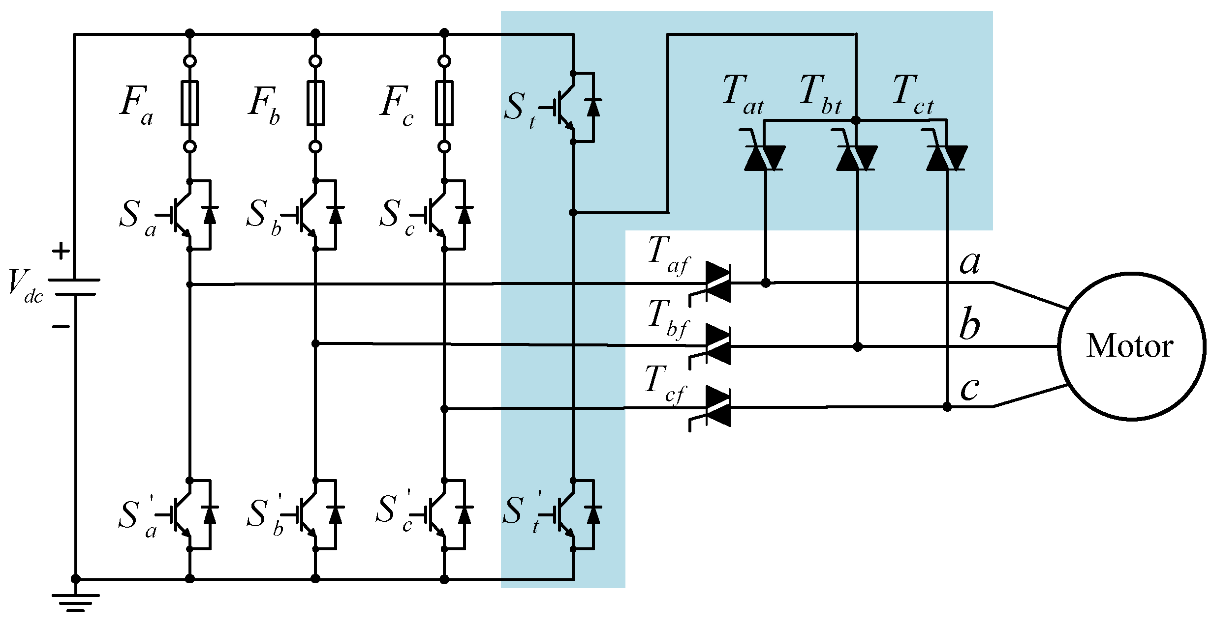
This research covers the situation when one power switch of the inverter is open- or short-circuited. The fault-tolerant inverter drive system is shown in Figure 1, which contains six IGBTs, $S_a$, $S_a^{\prime }$, $S_b$, $S_b^{\prime }$, $S_c$, and $S_c^{\prime }$, and two back-up IGBTs, $S_t$ and $S_t^{\prime }$. At the output of the inverter, six TRIACs, including $T_{at}$, $T_{bt}$, $T_{ct}$, $T_{af}$, $T_{bf}$, and $T_{cf}$ are added. In addition, three high-speed fuses $F_a$, $F_b$, and $F_c$ are inserted into the inverter and a back-up leg, including $S_t$ and $S_t^{\prime }$, is added as well. This paper discusses an open-circuit fault and a short-circuit fault of one leg in the inverter.

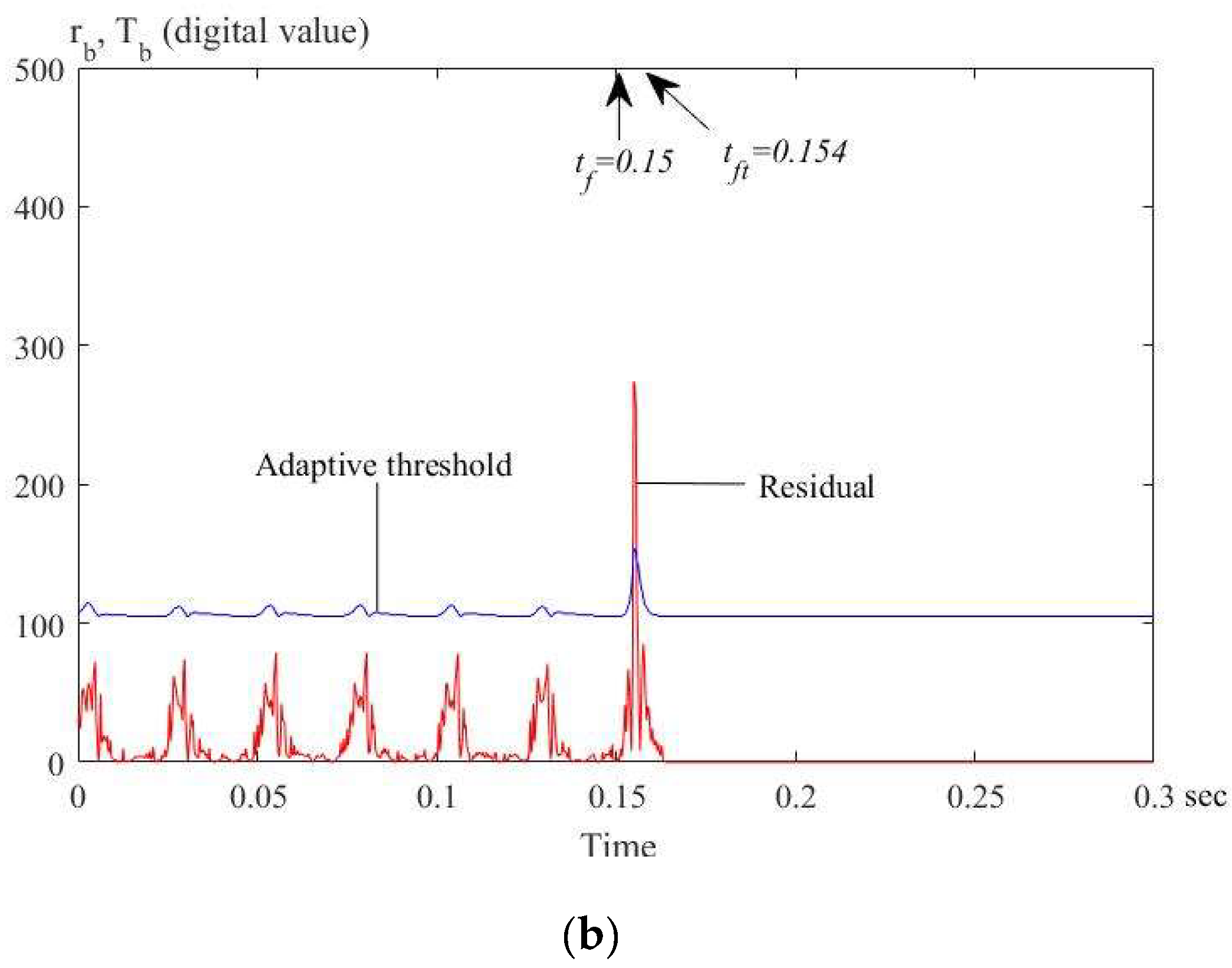
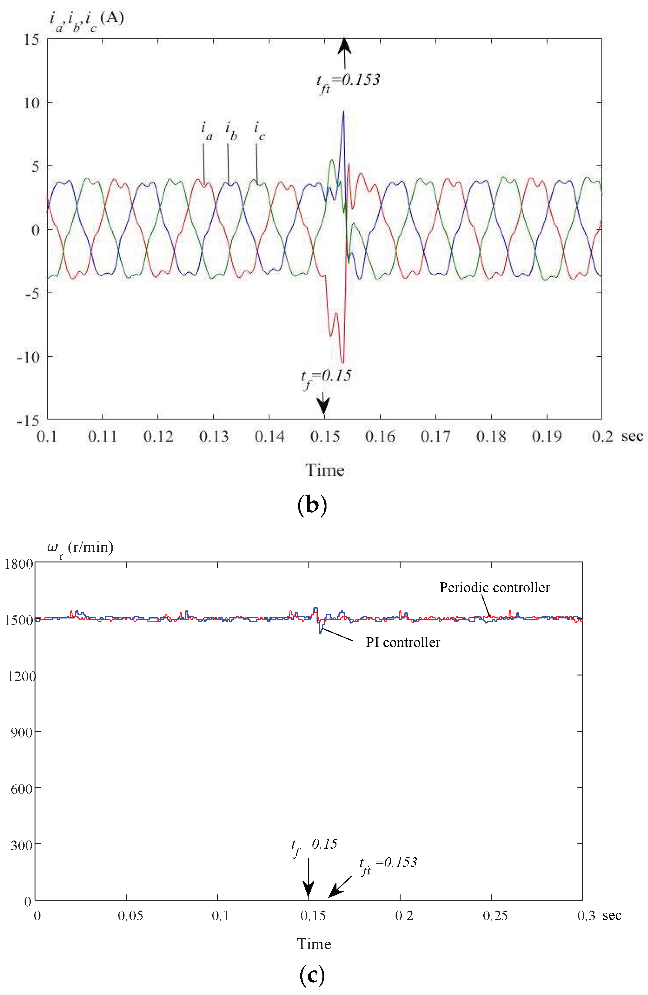
A performance index is established to identify if the SPMSM drive system failed [7]. During normal operation, the square magnitude error is calculated as follows:

$${\epsilon }_n(k)\cong {(\frac{v_d(k)}{L_s}\Delta t)}^2+{(\frac{v_q(k)-e_q(k)}{L_s}\Delta t)}^2,$$

(1)

where ${\epsilon }_n(k)$ is the performance index under normal conditions. $v_d(k)$ is the d-axis voltage, $L_s$ is the self-inductance, $v_q(k)$ is the q-axis voltage, $e_q(k)$ is the back-EMF, and $\Delta t$ is the time of each time interval. To avoid false detection, according to the authors’ experiences, 10 times the normal error vector is an adequate threshold to determine the faulty condition. The performance index in the faulty condition, $\epsilon (k)$ can be expressed as

$$\epsilon {(k)}_{}{>}_{}{10}_{}{\epsilon }_n^{}(k).$$

(2)

In Equation (2), the performance index of the SPMSM in a faulty condition, $\epsilon (k)$, can be defined as

$$\epsilon (k)=\Delta i_d^2(k)+\Delta i_q^2(k),$$

(3)

where $\epsilon (k)$ is the performance index in a faulty condition. $\Delta i_d(k)$ and $\Delta i_q(k)$ are the current deviations in the d-axis and q-axis in a faulty condition. The DSP diagnoses the faulty condition by measuring the deviations of the d-axis and q-axis currents and then identifying whether the faulty condition occurred in either the a-phase, b-phase, or c-phase. 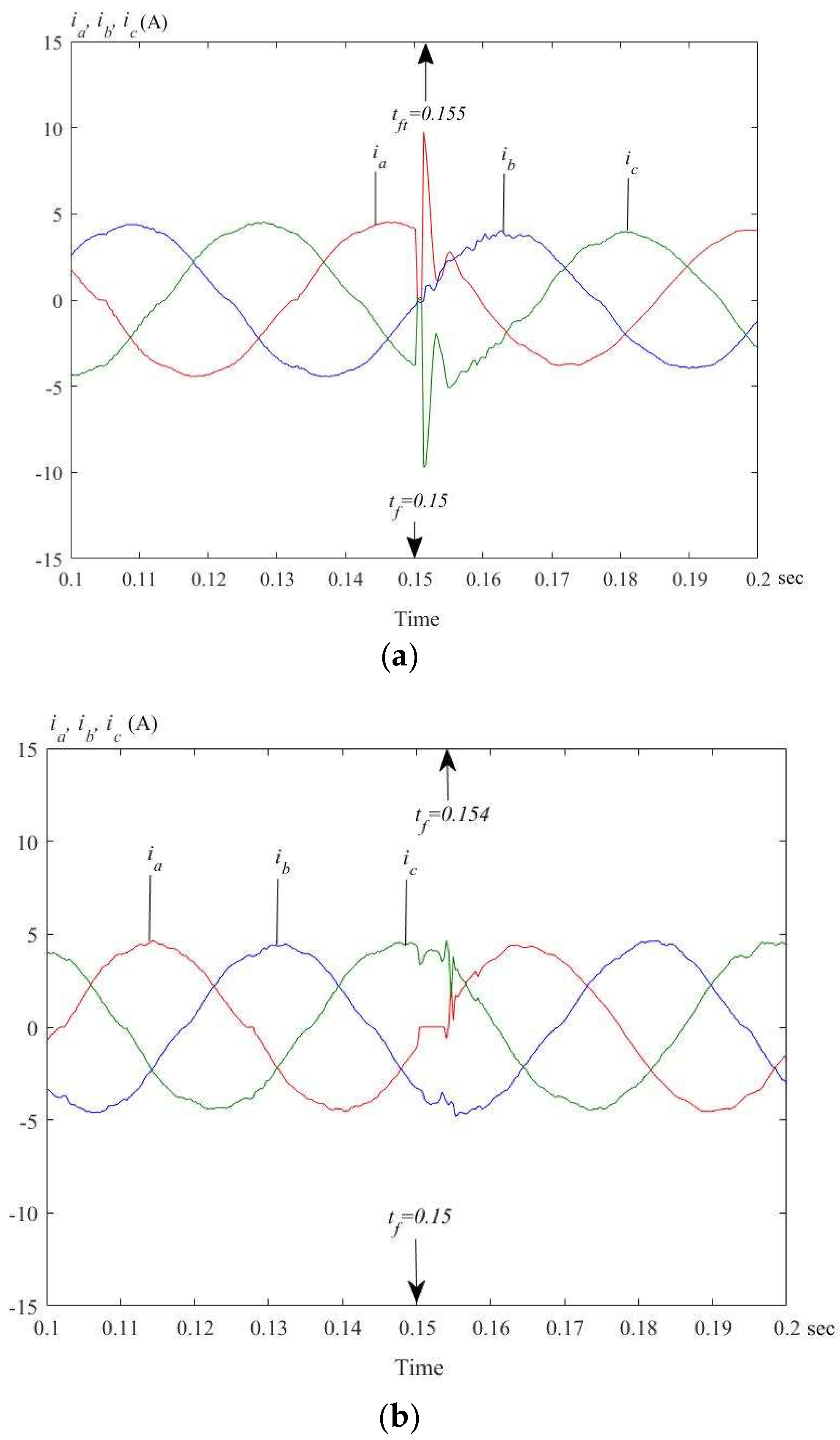The DSP transforms the a, b, c axis currents in the $\alpha$–$\beta$ axis currents, and then computes the current angle $\delta$ [21,22]. 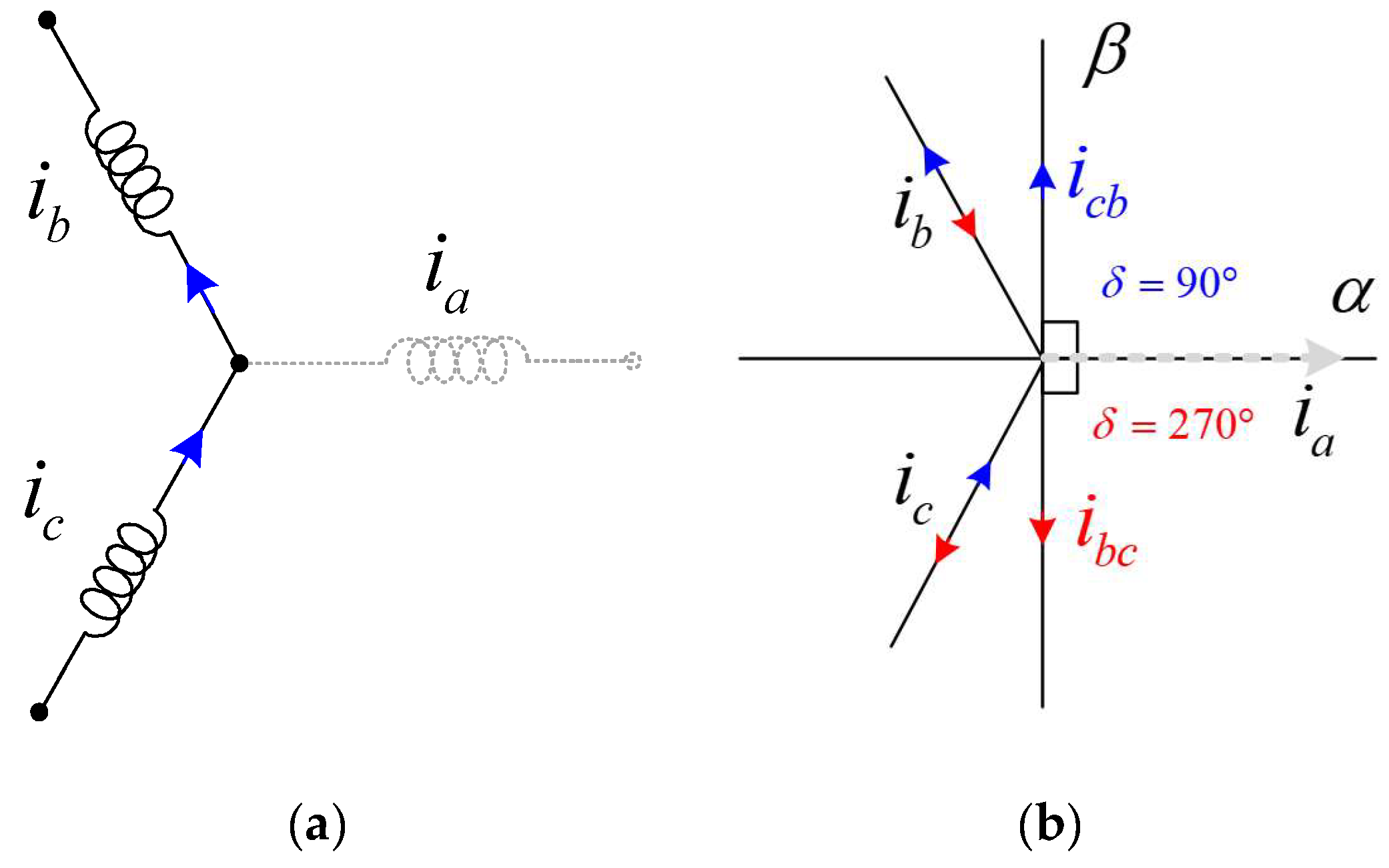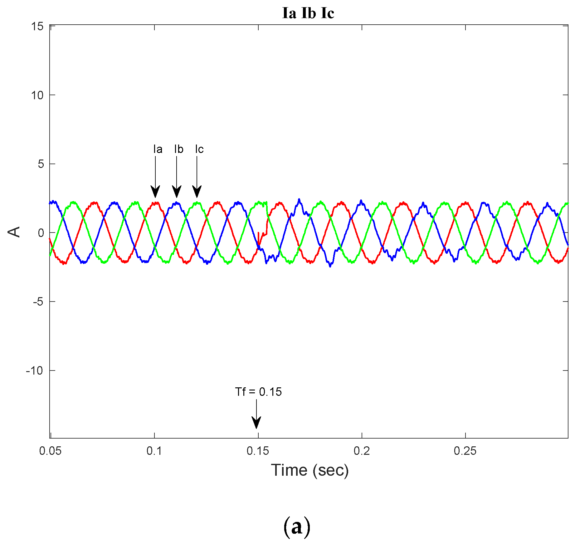Taking the a-phase fault as an example, Figure 2a shows the b-phase and c-phase currents when the a-phase winding is open-circuited. The current can flow in either direction as shown in Figure 2b. The current may flow from the b-phase to the c-phase, which results in the current vector having a 270$°$ angle, or the current may flow from the c-phase to the b-phase, which results in a 90$°$ angle. The summarized results of the current angle $\delta$ when one phase is faulty are shown in

Table 1. Current angle at different faulty phases.

Current Angle δ		Faulty Phase
Upper Quadrant	Lower Quadrant
90°	270°	a-phase
30°	210°	b-phase
150°	330°	c-phase

. By computing the current angle $\delta$, one can easily diagnose which phase is open. After that, an isolation and control method is executed to isolate the faulty part, and uses the back-up leg to replace the faulty leg. A fault-tolerant SPMSM drive system, thus, can be achieved.

2.2. Fault Detection and Control of a Current Sensor

This paper also investigates the detection and control of a fault in a one-phase current sensor. Previous research used a current estimator to evaluate the current sensor error, and an adaptive threshold was used to detect and diagnose the faulty condition [23,24]. In a faulty condition, the estimated current replaces the faulty current. The $\alpha$–$\beta$ axis voltages and currents were obtained using a coordinate transformation, and the estimated $\alpha$–$\beta$ currents in the discrete time domain can be expressed as

$${\widehat{i}}_{\alpha }\left(k\right)={\widehat{i}}_{\alpha }\left(k-1\right)+\frac{T_s}{L_s}\left[v_{\alpha }^{}\left(k\right)-r_s{i}_{\alpha }\left(k\right)-{\omega }_e\left(k\right){\lambda }_m\sin {\theta }_e\left(k\right)\right],$$

(4)

and

$${\widehat{i}}_{\beta }\left(k\right)={\widehat{i}}_{\beta }\left(k-1\right)+\frac{T_s}{L_s}\left[v_{\beta }^{}\left(k\right)-r_s{i}_{\beta }\left(k\right)+{\omega }_e\left(k\right){\lambda }_m\cos {\theta }_e\left(k\right)\right],$$

(5)

where ${\widehat{i}}_{\alpha }(k)$ and ${\widehat{i}}_{\beta }(k)$ are the estimated current, $v_{\alpha }(k)$ and $v_{\beta }^{}(k)$ are the $\alpha$–$\beta$ axis voltages, and $i_{\alpha }(k)$ and $i_{\beta }(k)$ are $\alpha$–$\beta$ axis currents. ${\omega }_e(k)$ and ${\theta }_e(k)$ are the electrical speed and angle. The current waveform factor $F_x(k)$ and ${\widehat{F}}_x(k)$ can be calculated as

$$F_x\left(k\right)=\frac{{\left|i_x\right|}_{\mathrm{RMS}}\left(k\right)}{{\left|i_x\right|}_{\mathrm{AVG}}\left(k\right)+e},$$

(6a)

and

$${\widehat{F}}_x\left(k\right)=\frac{{\left|i_x+{\epsilon }_x\right|}_{\mathrm{RMS}}\left(k\right)}{{\left|i_x+{\epsilon }_x\right|}_{\mathrm{AVG}}\left(k\right)+e},$$

(6b)

where e is a constant to prevent the denominator in the Equations (6a) and (6b) from reaching zero. $|i_x{|}_{RMS}(k)$ is the absolute value of the measured RMS current, $|i_x{|}_{AVG}(k)$ is the absolute value of the measured average current, and ${\epsilon }_x(k)$ is the estimated error. The residual function $R_x(k)$ is obtained by computing the difference between the estimated waveform factor ${\widehat{F}}_x(k)$ and the measured waveform factor $F_x(k).$ It can be expressed as

$$R_x\left(k\right)={\widehat{F}}_x\left(k\right)-F_x\left(k\right).$$

(7)

By substituting Equations (6a) and (6b) into Equation (7), the residual function $R_x(k)$ in the equation can be transformed into

$$R_x\left(k\right)=\frac{{\left|i_x+{\epsilon }_x\right|}_{\mathrm{RMS}}\left(k\right)}{{\left|i_x+{\epsilon }_x\right|}_{\mathrm{AVG}}\left(k\right)+e}-\frac{{\left|i_x\right|}_{\mathrm{RMS}}\left(k\right)}{{\left|i_x\right|}_{\mathrm{AVG}}\left(k\right)+e}=-\frac{{\left|i_x+{\epsilon }_x\right|}_{\mathrm{RMS}}\left(k\right)}{{\left|i_x+{\epsilon }_x\right|}_{\mathrm{AVG}}\left(k\right)+e}-\frac{{\left|i_x\right|}_{\mathrm{RMS}}\left(k\right)}{{\left|i_x\right|}_{\mathrm{AVG}}\left(k\right)+e},$$

(8)

where ${\epsilon }_x(k)$ is the estimated current error of the a, b, c phases. The numerator of the estimated absolute value of the RMS current $|i_x+{\epsilon }_x{|}_{RMS}(k)$ is always lower than or equal to the total of $|i_x{|}_{RMS}(k)+|{\epsilon }_x{|}_{RMS}(k)$ due to the triangular inequality rule. By using this relationship, the residual function $R_x(k)$ can be rewritten as

$$R_x\left(k\right)\le \frac{{\left|i_x\right|}_{\mathrm{RMS}}\left(k\right)}{{\left|i_x+{\epsilon }_x\right|}_{\mathrm{AVG}}\left(k\right)+e}+\frac{{\left|{\epsilon }_x\right|}_{\mathrm{RMS}}\left(k\right)}{{\left|i_x+{\epsilon }_x\right|}_{\mathrm{AVG}}\left(k\right)+e}-\frac{{\left|i_x\right|}_{\mathrm{RMS}}\left(k\right)}{{\left|i_x\right|}_{\mathrm{AVG}}\left(k\right)+e}.$$

(9)

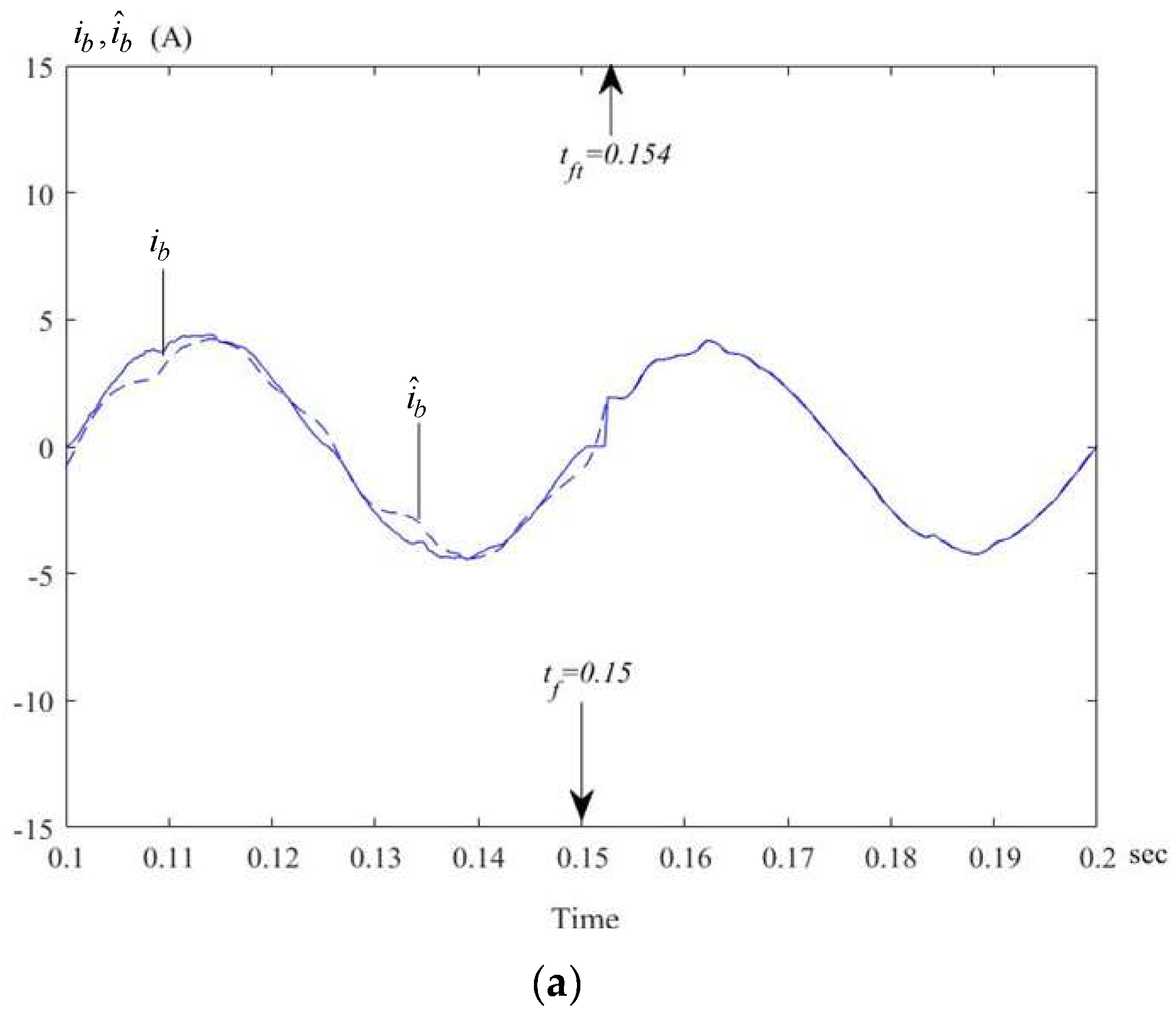
The difference between the threshold value and the residual value is used to determine if a faulty condition occurred. When the system is in a steady-state condition and the current sensor is in a normal condition, the measured and estimated waveform factors are constants and the residual value is near zero. On the other hand, when the current sensor is in a faulty condition, the residual value abruptly increases due to its large error. Finally, the estimated current ${\widehat{i}}_x(k)$ replaces the measured faulty current $i_x(k).$ However, in this paper, the estimated currents are near the measured currents only in steady-state conditions. The transient responses of the estimated currents are ignored to simplify the current estimating method.

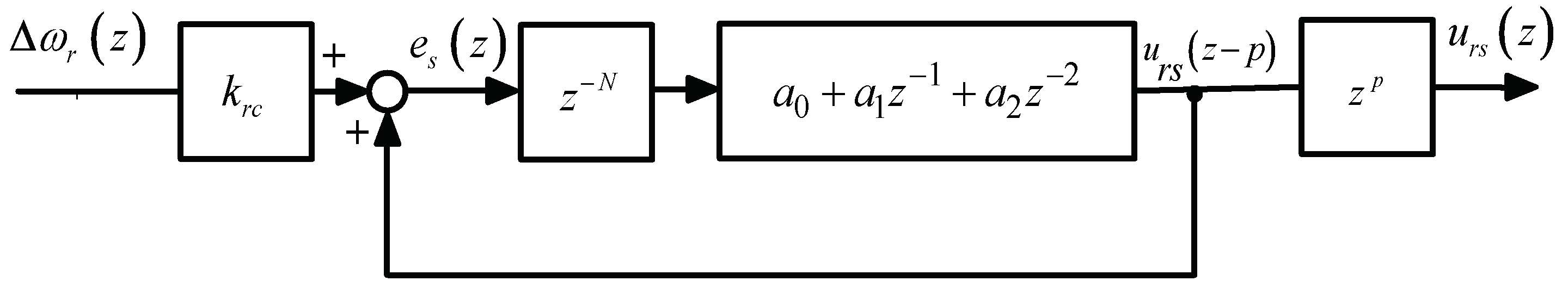
3. Speed-Loop Periodic Controller

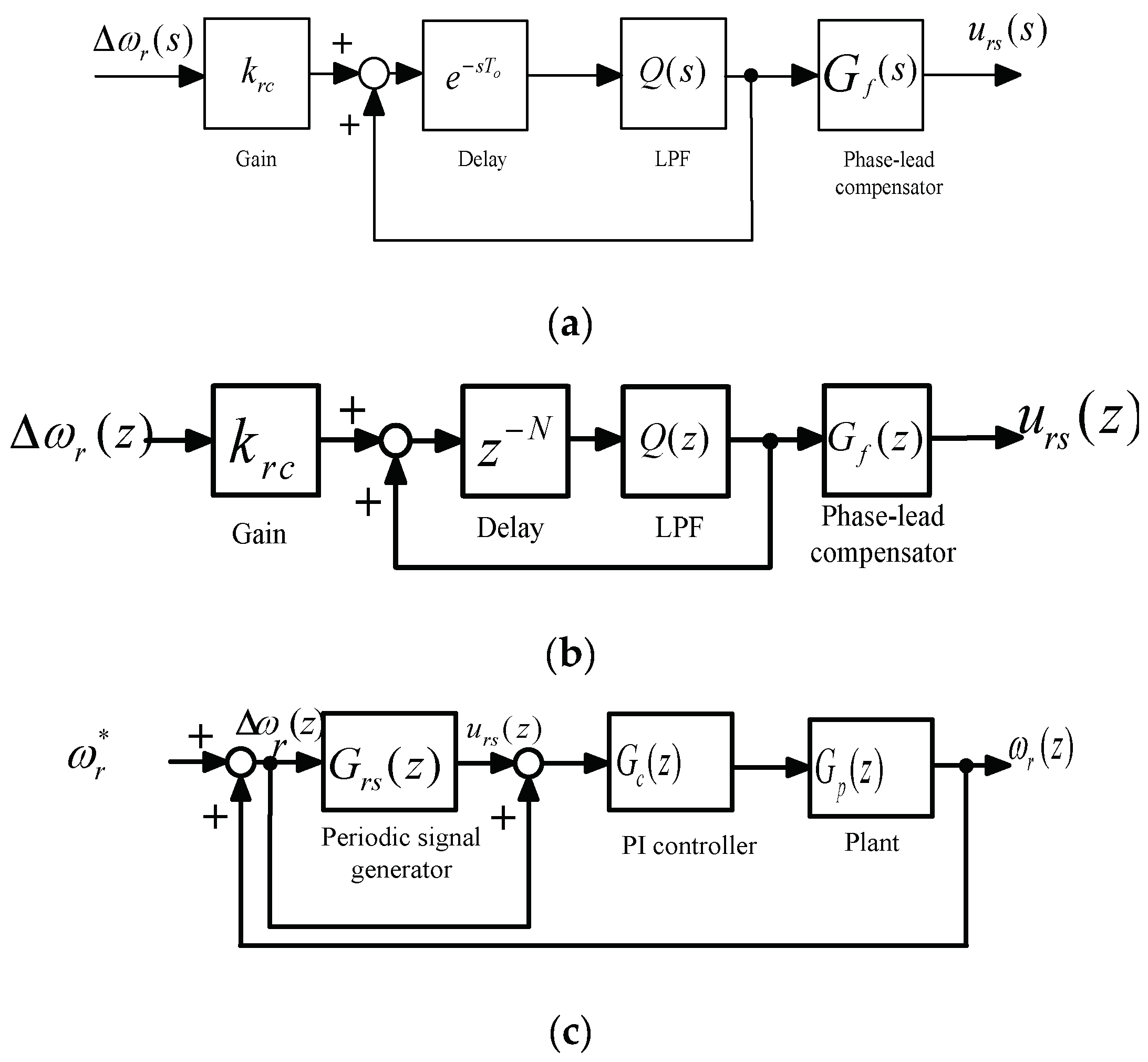
The speed-loop periodic controller for a fault-tolerant SPMSM in this paper is an original idea. The internal model principle states that perfect asymptotic tracking of persistent inputs can be attained by replicating the signal generator in a stable feedback loop [25]. The internal model of the inputs is a signal generator. Figure 3a shows the basic continuous s-domain structure of a periodic signal generator, which includes a delay device $e^{-s{T}_O}$ and a positive feedback. According to Figure 3a and assuming Q(s) = 1, the transfer function of the periodic signal generator can be expressed as

$$G_{rs}(s)=\frac{u_{rc}(s)}{e(s)}=\frac{e^{-s{T}_O}}{1-e^{-s{T}_O}},$$

(10)

where $G_{rs}(s)$ is the transfer function of the periodic signal generator, and $e^{-s{T}_O}$ is a time-delay unit. From Equation (10), the periodic signal generator $G_{rs}(s)$ can be expanded as follows [26]:

$$G_{rs}(s)=\frac{e^{-s{T}_O}}{1-e^{-s{T}_O}}=-\frac{1}{2}+\frac{1}{s{T}_O}+\frac{1}{T_O}{\displaystyle \sum _{n=1}^{\infty }\frac{2s}{s^2+{(n{\omega }_o)}^2}}.$$

(11)

In Equation (11), the first item is a transfer function of an impulse, the second item is a transfer function of a step input, and the third item is the transfer function of the harmonics. In the real world, a low-pass filter Q(s) is required to compensate for the related harmonics, and a phase-lead compensator $G_f(s)$ is used for the entire system delay compensation. To simplify the problem, assuming $Q(s)$ is 1, the classic periodic controller makes $G_{rs}(s)$ approach $\infty$ at poles s = $\pm jn{\omega }_o.$ In this research, a DSP is used to execute the control algorithm; as a result, the s-domain periodic signal generator needs to convert into the z-domain periodic signal generator shown in Figure 3b. The z-domain periodic signal generator is expressed in a discrete form as follows:

$$G_{rs}\left(z\right)=k_{rc}\frac{Q\left(z\right)z^{-N}}{1-Q\left(z\right)z^{-N}}{G}_f\left(z\right),$$

(12)

where $k_{rc}$ is a constant control gain, $Q(z)$ is a low-pass filter (LPF), $G_f(z)$ is a phase-lead compensator that compensates for the time delay, and N is the number of delay steps.

In the discrete time domain, the $z^{-N}$ is added as shown in Figure 3b. N can be expressed as

$$N=\frac{T_0}{T_s},$$

(13)

where $T_0$ is the fundamental period and $T_s$ is the sampling interval of the speed-loop control system. The fundamental period $T_0$ determines the delay of the periodic controller in N steps. The delay steps determine the settling time of the SPMSM drive system. If the delay time is set too short, the output generates obvious overshoot but has quick responses; however, if the delay time is too long, the periodic controller has slow responses. The choice of the parameter N depends on the designer’s experience. In addition, the periodic controller is added into the speed-loop PI controller in the forward loop [26], which is shown in Figure 3c. The speed-loop PI controller is used to improve the transient responses and load disturbance responses for the normal operation speed dynamics; however, the speed-loop periodical controller is used when the SPMSM drive system is faulty, which causes three-phase current imbalance. In Figure 3c, $G_p(z)$ is the transfer function of the SPMSM drive system, $G_c(z)$ is the speed-loop PI controller, and $G_{rs}(z)$ is the periodic signal generator, which is used to reduce the current harmonics. After that, the speed command ${\omega }_r{}^{*}$ is input into the closed-loop system. In this closed-loop system, a periodic signal output $u_{rs}(z)$ is added to the speed error $\Delta {\omega }_r(z)$ to generate the total input of the PI controller to control the system.

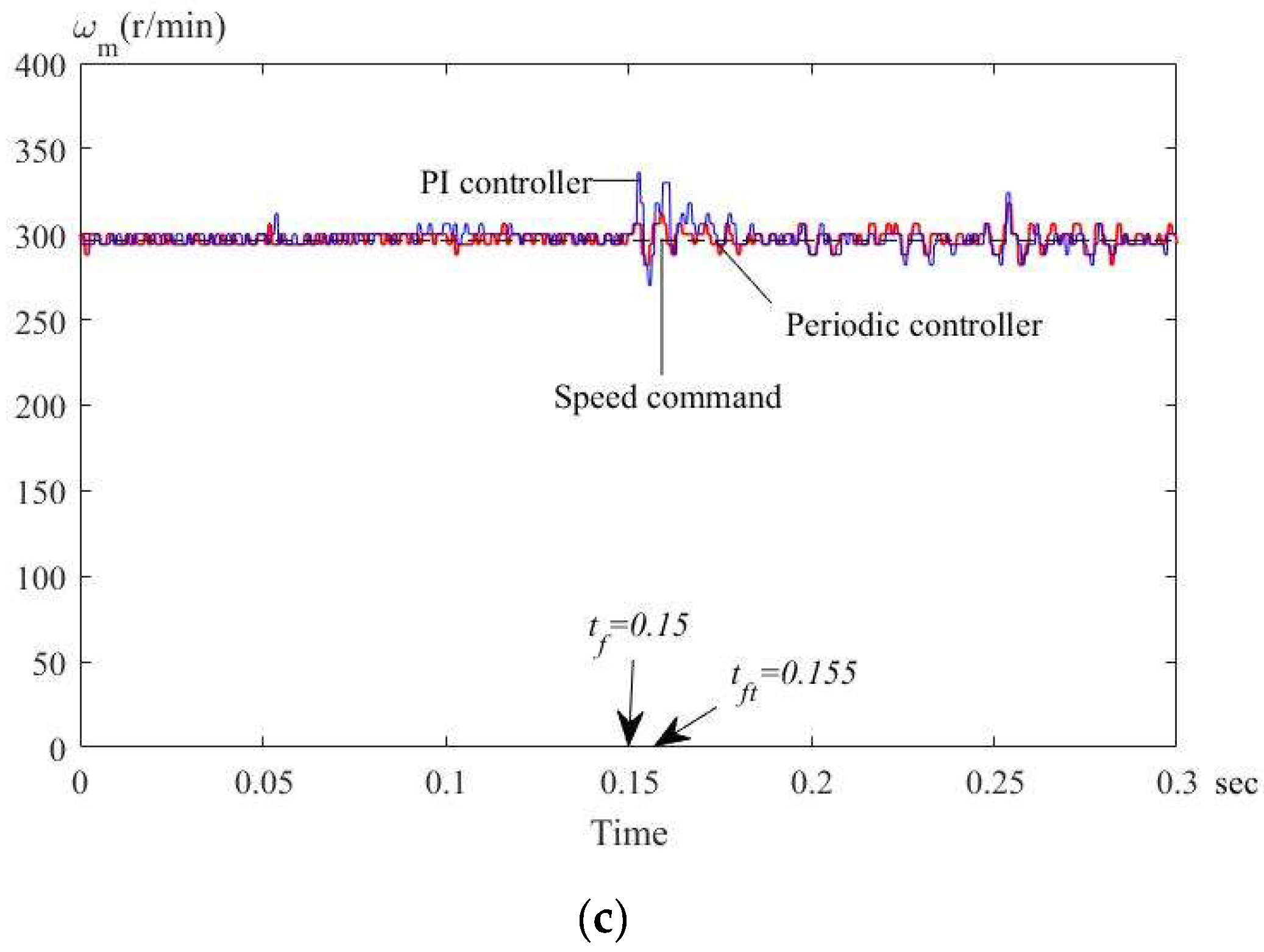
Compared to the traditional speed-loop PI controller, the proposed method uses a periodic controller to cascade to the traditional speed-loop PI controller, which increases the gain at certain frequencies. As a result, the transient responses and load disturbance responses of the SPMSM can be effectively improved. The computation of the periodic controller is very simple, which only includes a delay operation, a low-pass filter, a positive feedback operation, and phase-lead compensation. As a result, it is easy to implement the proposed control method by using a DSP.

The parameters of the periodic controller, including a control gain $k_{rc}$ and a phase-lead compensation $G_f(z)$, are determined by using stability analysis in the closed-loop control system. The detailed analysis and the stable condition of a closed-loop control system were previously discussed and can be expressed as follows [13]:

$$k_{rc}^{}<\frac{2\cos ({\theta }_H+p\omega )}{\left|H(e^{j\omega })\right|}\mathrm{and}{k}_{rc}^{}\ge 0,$$

(14a)

and

$$H(z)=\frac{G_c(z)G_p(z)}{1+G_c(z)G_p(z)},$$

(14b)

where ${\theta }_H$ is the phase angle of H(z), $\omega$ is the frequency, p is the order of the phase-lead compensation, and $H(z)$ is the transfer function of the closed-loop control system. The control gain $k_{rc}$ and the order $p$ of the phase-lead compensation are determined as shown below. In the z-domain analysis, the phase-lead compensation $G_f(z)$ is commonly expressed as follows [13]:

$$G_f\left(z\right)=z^p$$

(15)

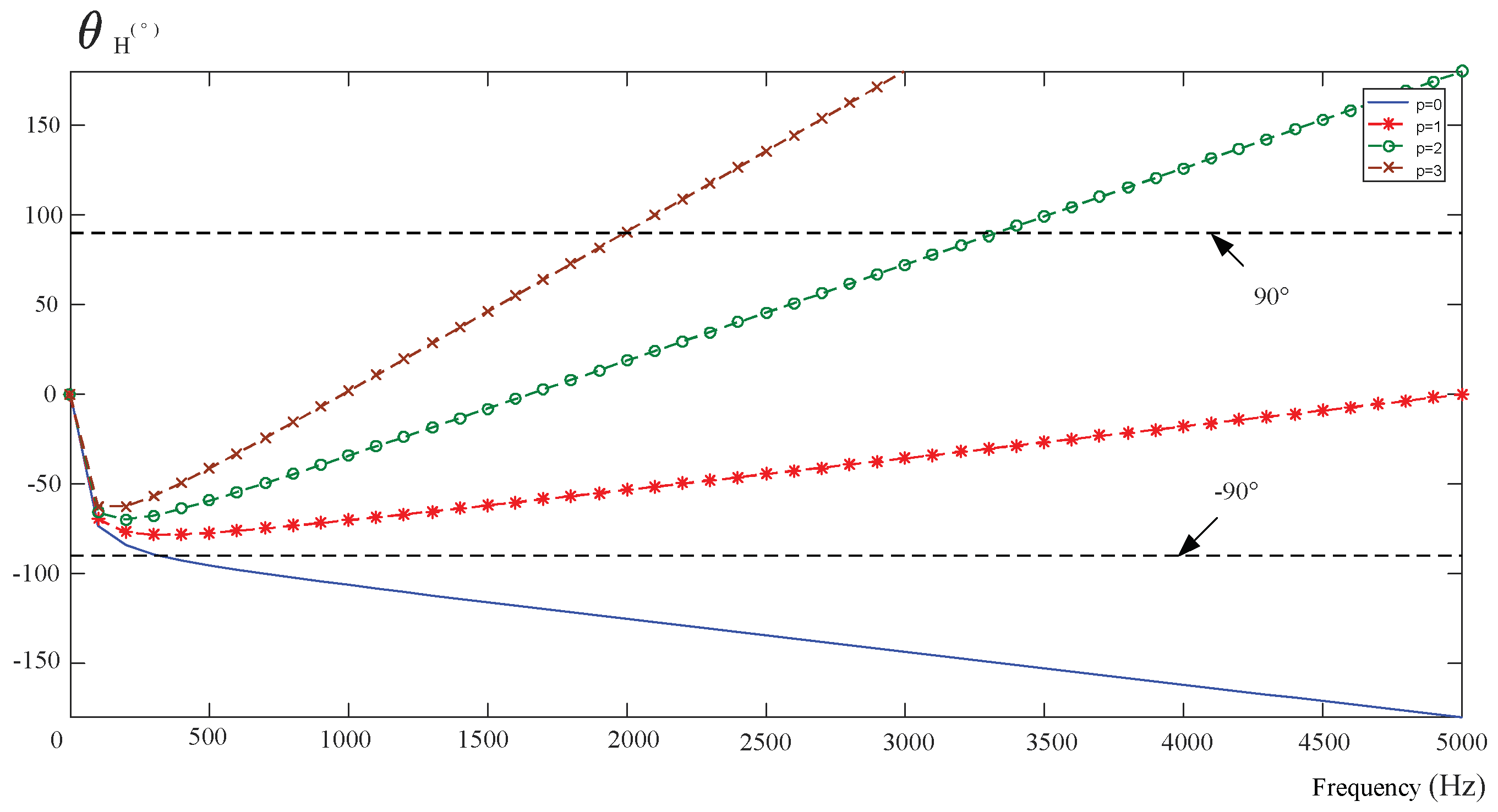
The characteristics of the closed-loop speed-control SPMSM drive system are discussed here. Figure 4 shows the relationship between the boundary of the phase angle and operating frequency of the closed-loop drive system. The phase lead step p includes steps 0, 1, 2, and 3, which are shown as p = 0, p = 1, p = 2, and p = 3 in Figure 4, respectively. In the physical system, the available range of the compensated phase is between −${90}^{\mathrm{o}}$ and $90^{\mathrm{o}}$, which is shown as the dashed line in Figure 4. From Figure 4, to operate in the phase boundary between −${90}^{\mathrm{o}}$ and ${90}^{\mathrm{o}}$, the maximum operating frequency is 0.4 kHz for zero-step phase-lead compensation, 5 kHz for one-step phase-lead compensation, 3.3 kHz for two-step phase-lead compensation, and 1.9 kHz for three-step phase-lead compensation. In order to obtain the widest operating frequency of the closed-loop SPMSM drive system, the one-step phase lead (p = 1) is selected in this research. 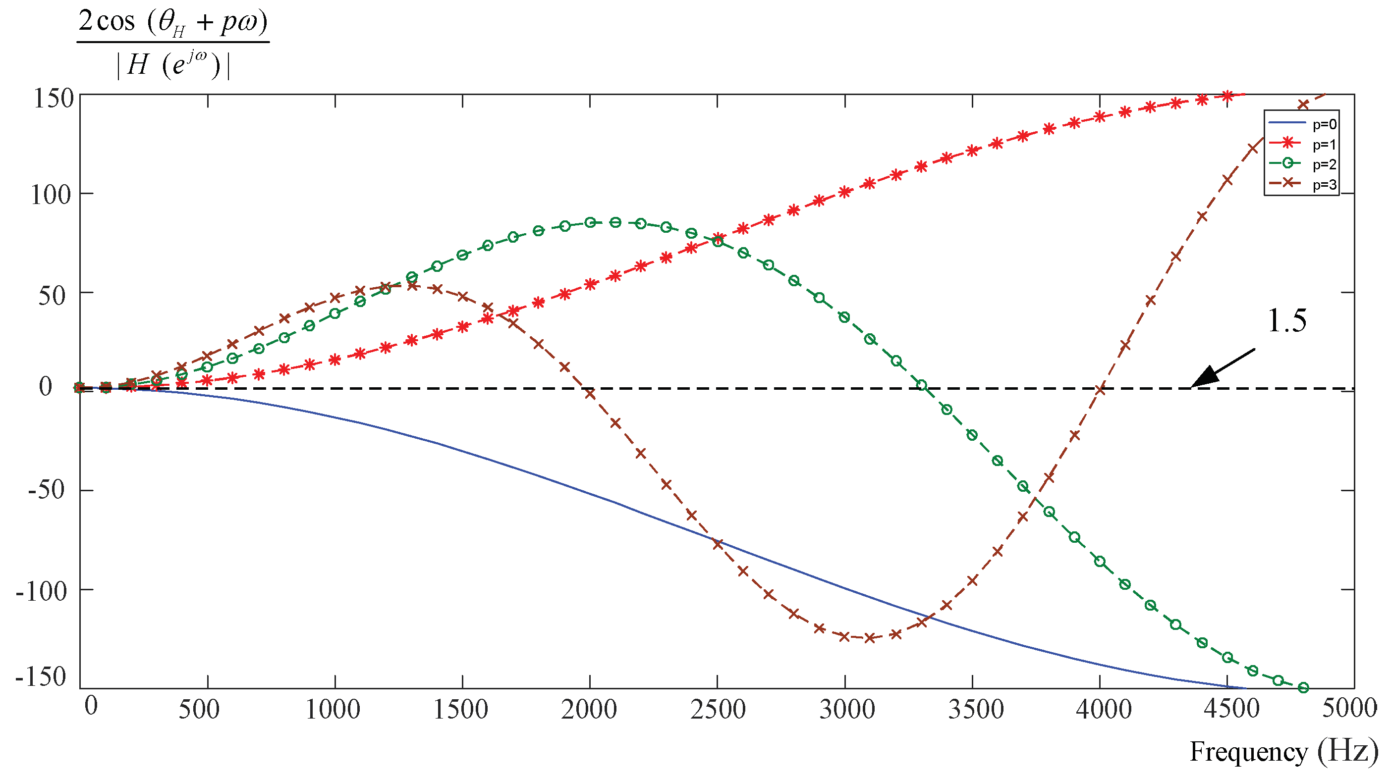After that, the gain $k_{rc}$ is chosen according to the stability analysis. The stability condition is shown in Equation (14a), which shows that the gain $k_{rc}$ needs to satisfy the inequality equation. Figure 5 shows the relationship between the maximum boundary $\frac{2\cos ({\theta }_H+p\omega )}{\left|H(e^{j\omega })\right|}$ and the operation frequency. In order to both satisfy Equation (14a) and obtain the widest operating frequency range, the one-step phase-lead compensation that provides a very smooth curve was chosen for this paper. By using the one-step phase-lead compensation and satisfying Equation (14a), $k_{rc}$ was selected as 1.5 because $\frac{2\cos ({\theta }_H+p\omega )}{\left|H(e^{j\omega })\right|}$ was varied between 1.5 and 150 when the operating frequency varied from 0 kHz to 5 kHz.

The low-pass filter, LPF $Q^{}(z)$, was designed by using finite impulse response (FIR). FIR was chosen here because it is commonly used in digital filter applications. The transfer function of an FIR LPF $Q^{}(z)$ can be expressed as

$$Q(z)={\displaystyle \sum _{i=0}^m{a}_i{z}^{-i}}.$$

(16)

The components of the periodic controller are shown in Figure 6. The speed error $\Delta {\omega }_e(z)$ is multiplied with a control gain $k_{rc}$, and then added to the $z^{-p}{u}_{rs}(z)$ to generate $e_s(z)$. A low-pass filter, $a_0+a_1{z}^{-1}+a_2{z}^{-2}$, is used to reduce the high-frequency noise. After that, the output of the low-pass filter, which is $z^{-p}{u}_{rs}(z)$, is added to the $k_{rc}\Delta {\omega }_r\left(k\right)$ to obtain $e_s(z).$ Finally, $u_{rs}(z-p)$ passes through the phase-lead compensator $z^p$ to obtain the $u_{rs}(z)$. By using k as the interval step number, the output before delay is expressed as $u_{rs}(z)z^{-p}$, and then the system error $e_s(z)$ can be transformed into

$$e_s\left(k\right)=k_{rc}\Delta {\omega }_r\left(k\right)+u_{rs}\left(k-p\right).$$

(17)

By using the LPF $Q^{}(z)$ with $a_i$ as the coefficient, the $u_{rc}(k)$ can be expressed as

$$u_{rs}\left(k\right)={\displaystyle \sum _{i=0}^m{a}_i{e}_s\left(k-N-i+p\right)}{,}_{ }i=0,1,2.$$

(18)

The total of $u_{rs}(k)$ and $\Delta {\omega }_r(z)$ becomes the control input of the PI controller.

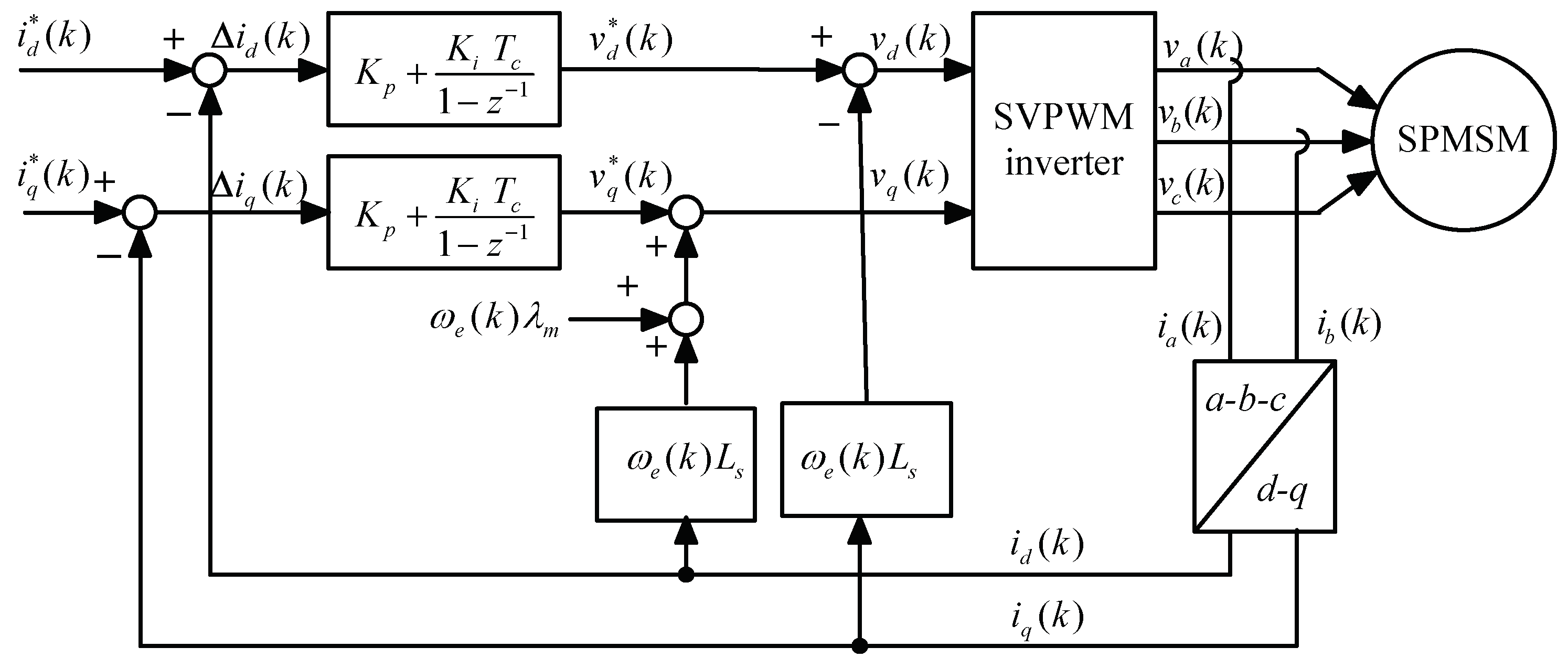
4. Current-Loop Controller

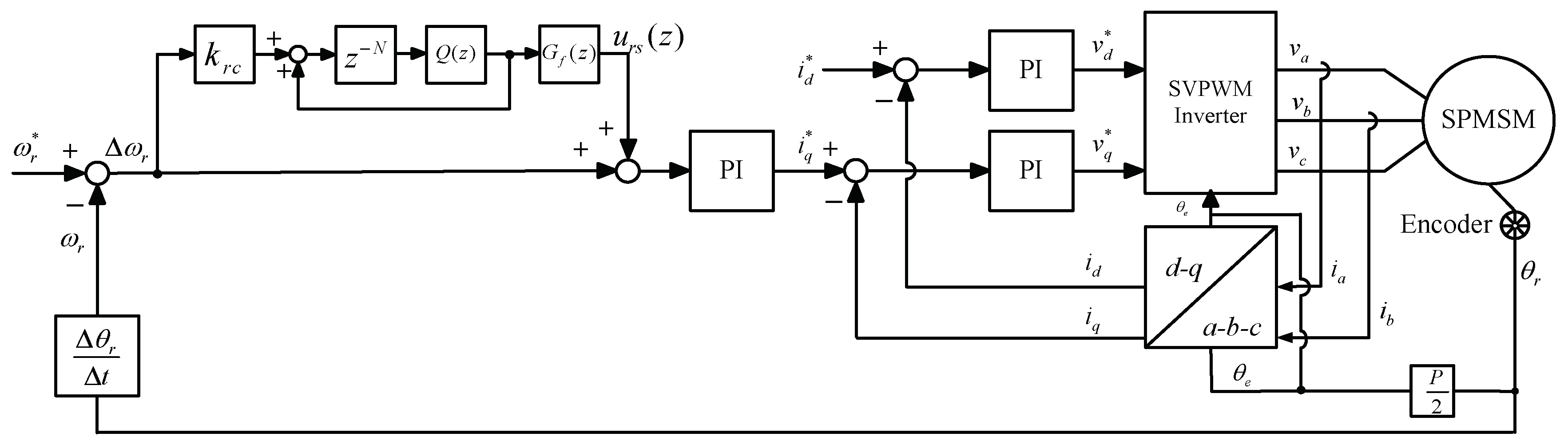
In general, the current-loop PI controller, which is a minor-loop of the SPMSM drive system, is cascaded with the speed-loop controller. Figure 7 shows the detailed block diagram of the speed-loop controller and current-loop controller in an SPMSM drive system. First, the speed ${\omega }_r$ is subtracted from the speed command ${\omega }_r^{*}$ to obtain the speed error $\Delta {\omega }_m$. Then, the speed-loop controller is executed to generate the q-axis current command $i_q^{*}$. The d-axis current command is set at zero in this research. Next, two PI controllers are designed to compute the d-axis voltage command $v_d^{*}$ from the d-axis current error, and also the q-axis voltage command $v_q^{*}$ from the q-axis current error. After that, the SVPWM inverter generates a-, b-, c-axis voltages $v_a$, $v_b$, and $v_c$ from the information of the $v_d^{*}$, $v_q^{*}$, and electrical rotor position ${\theta }_e$. The a, b, c voltages are injected into the SPMSM to generate the a, b, c currents $i_a$, $i_b$, and $i_c$. Finally, the SPMSM rotates and reports its mechanical angle ${\theta }_m$ to the DSP.

The SPMSM drive system returns the signals from the encoder and two Hall-effect current sensors to the DSP. The encoder detects the rotor angle ${\theta }_m$, and then computes the electrical angle ${\theta }_e$ by multiplying pole pairs. The rotor speed ${\omega }_r$ is obtained by taking the difference operation from the ${\theta }_r$. Two Hall-effect current sensors are used to measure the a-phase and b-phase currents $i_a$ and $i_b$, and then the c-phase current $i_c$ can be calculated because it is a three-phase balanced system. The relationship between the a, b, c currents and the d-, q-axis currents is shown below.

$$\left[\begin{array}{c}{i}_d\\ i_q\end{array}\right]=\frac{2}{3}\left[\begin{array}{c}\begin{array}{ccc}\cos ({\theta }_e)& \cos ({\theta }_e-\frac{2\pi }{3})& \cos ({\theta }_e+\frac{2\pi }{3})\end{array}\\ \begin{array}{ccc}\sin ({\theta }_e)& \sin ({\theta }_e-\frac{2\pi }{3})& \sin ({\theta }_e+\frac{2\pi }{3})\end{array}\end{array}\right]\left[\begin{array}{c}{i}_a\\ i_b\\ i_c\end{array}\right].$$

(19)

In the d-, q-axis synchronous frame, the dynamic equation of currents for an SPMSM is expressed as

$$\frac{d{i}_d(t)}{dt}=\frac{1}{L_s}\left(v_d(t)-r_s{}_{}{i}_d(t)+{\omega }_e{(t)}_{}{L}_s{}_{}{i}_q(t)\right),$$

(20)

$$\frac{d{i}_q(t)}{dt}=\frac{1}{L_s}\left(v_q(t)-r_s{}_{}{i}_q(t)-{\omega }_e{(t)}_{}{L}_s{}_{}{i}_d(t)-{\omega }_e{(t)}_{}{\lambda }_m\right).$$

(21)

The dynamic equation of the speed is

$$\frac{d{\omega }_e(t)}{dt}=\frac{1}{J_m}\left(T_e-B_m{\omega }_e(t)-T_L\right),$$

(22)

and the electromagnetic torque is

$$T_e=\frac{3}{2}\frac{P}{2}\left({\lambda }_m{}_{}{i}_q(t)\right),$$

(23)

where $\frac{d}{dt}$ is the differential operator, $L_s$ is the stator inductance, $r_s$ is the stator resistance, ${\lambda }_m$ is the flux linkage, $J_m$ is the inertia, $B_m$ is the friction coefficient, and $T_L$ is the external load. Assuming the resistance voltage is neglected and the decoupling forward method is used, then the d-, q-axis voltage $v_d^{*}$ and $v_q^{*}$ can be expressed as

$$\frac{1}{L_s}{v}_d^{*}=\frac{1}{L_s}\left(v_d+{\omega }_e{L}_s{i}_q\right),$$

(24)

and

$$\frac{1}{L_s}{v}_q^{*}=\frac{1}{L_s}\left(v_q-{\omega }_e{L}_s{i}_d-{\omega }_e{\lambda }_m\right).$$

(25)

Substituting Equations (24) and (25) into Equations (20) and (21), the dynamics of the SPMSM can be rewritten as

$$\frac{d{i}_d}{dt}=-\frac{r_s}{L_s}{i}_d^{}+\frac{1}{L_s}{v}_d^{*},$$

(26)

and

$$\frac{d{i}_q}{dt}=-\frac{r_s}{L_s}{i}_q^{}+\frac{1}{L_s}{v}_q^{*}.$$

(27)

After using the current-loop PI controllers, the d-, q-axis voltage commands, $v_d^{*}$ and $v_q^{*}$, are expressed as

$$v_d^{*}(t)=K_P\left(i_d^{*}(t)-i_d(t)\right)+K_I{\displaystyle {\int }_0^t{\left(i_d^{*}(\tau )-i_d(\tau )\right)}_{}}d\tau ,$$

(28)

and

$$v_q^{*}(t)=K_P\left(i_q^{*}(t)-i_q(t)\right)+K_I{{\displaystyle {\int }_0^t\left(i_q^{*}(\tau )-i_q(\tau )\right)}}_{}d\tau .$$

(29)

The d-axis voltage is obtained by substituting Equation (28) into Equation (24), and the q-axis voltage is obtained by substituting Equation (29) into Equation (25). Finally, the output voltages can be expressed as

$$v_d^{}(t)=K_P\left(i_d^{*}(t)-i_d(t)\right)+K_I{{\displaystyle {\int }_0^t\left(i_d^{*}(\tau )-i_d(\tau )\right)}}_{}d\tau -{\omega }_e(t)L_s{i}_q(t),$$

(30)

and

$$v_q^{}(t)=K_P\left(i_q^{*}(t)-i_q(t)\right)+K_I{{\displaystyle {\int }_0^t\left(i_q^{*}(\tau )-i_q(\tau )\right)}}_{}d\tau +{\omega }_e(t)L_s{i}_d+{\omega }_e(t){\lambda }_m.$$

(31)

After transferring the continuous time domain into discrete time domain, one can obtain the d-, q-axis voltage commands as

$$v_d^{}(k)=K_P\left(i_d^{*}(k)-i_d(k)\right)+K_I{T}_c{\displaystyle \sum _{n=1}^k}{\left(i_d^{*}(k)-i_d(k)\right)}_{}-{\omega }_e{(k)}^{}{L}_s{}^{}{i}_q(k),$$

(32)

and

$$v_q^{}(k)=K_P\left(i_q^{*}(k)-i_q(k)\right)+K_I{}^{}{T}_c{\displaystyle \sum _{n=1}^k}\left(i_q^{*}(k)-i_q(k)\right)+{\omega }_e{(k)}^{}{L}_s{}^{}{i}_d(k)+{\omega }_e{(k)}^{}{\lambda }_m,$$

(33)

where $T_c$ is the sampling interval of the current loop. From Equations (32) and (33), a block diagram of the PI current-loop controller can be constructed as shown in Figure 8. In this research, the parameters of the PI controller were obtained by using the pole assignment technique.

5. Implementation

A block diagram of the implemented SPMSM drive system is shown in Figure 9a. A DSP type TMS320F2808 was used as the control center. The SPMSM drive system includes a fault-tolerant inverter, a DSP, gate drivers, current-sensing circuits, an encoder circuit, and an overcurrent protection circuit. The speed-loop PI controller includes $K_p=0.5$ and $K_I=0.2$, which are obtained by pole assignment with two poles, $p_1=0.79$ and $p_2=0.93$. The speed-loop periodic controller includes $k_{rc}=1.5$, $Q(z)=0.2+0.45z^{-1}+0.2z^{-2}$, N = 50, and $G_f(z)=z$. The sampling interval of the speed loop is 1 ms. The current-loop PI controllers include $K_p=12.17$ and $K_I$ = 0.0006, which determine the inner-loop current dynamics. The sampling interval of the current loop is 100 $\mathsf{\mu }\mathrm{s}.$

The SPMSM has the following parameters: $r_s{=}_{}$ ${0.73}_{}\mathsf{\Omega },$ $L_s=$ ${1.37}_{}{\mathrm{mH}}_{}$, ${\lambda }_m=$ ${0.167}_{}\mathrm{Wb},$ $B_m=$ 0.003 N∙m∙s/rad, and $K_T=$ 1.0 N∙m/A. Figure 9b shows a photograph of the implemented drive system, which includes an SPMSM and a dynamometer, which provides the external load for the SPMSM drive system.

6. Simulated and Experimental Results

The simulated and experimental results were measured under the following five conditions: a normal condition, an open-circuit condition, a short-circuit condition, a faulty current sensor condition, and a multiple faulty condition. The details are given below.

6.1. Normal Condition Experimental Results

Figure 10a shows the measured speed responses at 100 r/min, 300 r/min, and 500 r/min. The periodic controller has quicker transient responses than the PI controller. Figure 10b shows the measured q-axis currents. The periodic controller provides greater input power when compared to the PI controller. Figure 11a shows the speed responses at 500 r/min when an external load of 3.5 N∙m was added. The periodic controller provides a lower speed drop and quicker recovery time than the PI controller. Figure 11b shows the q-axis current responses in the same case. The periodic controller shows better performance than the PI controller, including a lower overshoot and quicker recovery time when an external load is added.

6.2. Inverter Open-Circuit Faulty Condition Experimental Results

Figure 12a–c show the simulated results of the a-phase open circuit at 300 r/min without using the fault-tolerant method. The simulated results include the three-phase currents, q-axis current, and speed. Figure 13a shows the measured three-phase currents without using the proposed fault-tolerant method of the SPMSM drive system when its a-phase upper leg was open-circuited at 300 r/min. The faulty condition occurs at 0.15 s. A manual switch was in series with the power device. When the switch was opened, the power device was instantaneously opened. Thus, the PMSM drive system became a three-phase unbalanced drive system. Figure 13b shows the q-axis current response when the a-phase upper leg is open. The q-axis current oscillated due to the unbalanced three-phase currents. Figure 13c shows the measured speed response. As we can observe, in this figure, the speed varied between 485 r/min to 510 r/min when the a-phase upper leg was open. Figure 14a–c show the simulated results using the fault-tolerant control when the a-phase leg was open-circuited. The d-axis inductance remained the same as its nominal value, but the q-axis inductance was reduced to 50% of its nominal value due to the influence of saturation. The simulated results include the currents of the speed-loop PI controller, the currents of the speed-loop periodic controller, and the speed responses of speed-loop PI and periodic controllers. Figure 15a–c show the measured results of fault-tolerant control at 300 r/min when the a-phase was open-circuited. The periodic controller had better performance than the PI controller, including lower peak current and smaller speed variations during faulty intervals. Figure 15a shows the three-phase currents using the fault-tolerant method. Figure 15b shows the measured currents of the speed-loop periodic controller. The measured speed responses of both the PI controller and periodic controller are shown in Figure 15c. Figure 16a–c show the measured results of the fault-tolerant control when one switch of the a-phase leg was open-circuit at 1500 r/min.

6.3. Inverter Short-Circuit Faulty Condition Experimental Results

Figure 17a–c show the simulated results of the a-phase short-circuited at 300 r/min without using the fault-tolerant method, including the three-phase currents, q-axis current, and speed response. Figure 18a–c show the measured results of the same case. Figure 18a shows the measured three-phase currents without using the fault-tolerant method. Figure 18b shows the measured q-axis current. Figure 18c shows the measured speed response that dropped quickly due to the trip of the inverter. Figure 19a–c show the simulated results of the a-phase short-circuited at 300 r/min using the fault-tolerant method. The simulated results include the current responses, speed responses, and performance index. Figure 20a–c show the measured results of the fault-tolerant control when the a-phase inverter was short-circuited at 300 r/min. The two power devices in the upper leg and lower leg were both turned on to have this leg short-circuited. Figure 20a shows the measured current responses when using a PI controller. Figure 20b shows that the measured speed variation was 80 r/min when using a speed PI controller, but it was 50 r/min when using the speed-loop periodic controller. These results show that the periodic controller has better transient response than the PI controller. Figure 20c shows the performance index before and after the fault. Yan et al. proposed a PWM voltage source inverter diagnosis method for a PMSM drive system based on a fuzzy logic approach [27]. By using the fuzzy logic diagnosis method, the DSP could identify the faulty condition in 0.09 s after the fault occurrence. Compared to Yan’s method, in this paper, from Figure 20b, the short-circuit fault-tolerant control was finished in 0.01 s. As a result, this work reduced the time by approximately 89% when compared to Yan’s method. The reason is that fuzzy logic is more complicated than the method proposed in this paper. Hang et al. proposed the detection and discrimination of an open-phase fault in an SPMSM drive system based on the zero-sequence voltage components [28]. For one switch open, Hang’s proposed detection and discrimination method required 0.04 s. Compared to Hang’s method, in this paper, from Figure 15c, the open-circuit fault-tolerant control was finished in 0.006 s. As a result, this work reduced the time by approximately 85% when compared to Hang’s method. However, this paper may cause more conduction loss because six TRIACs were used to change the structure of the inverter. Figure 21a–c show the measured results of the short-circuit fault-tolerant control at one switch of the a-phase leg at 1500 r/min.

6.4. Current Sensor Faulty Condition Experimental Results

In addition, when the a-phase Hall-effect current sensor is open, the a-phase measured current suddenly becomes zero. Then, the estimated current is used to replace the measured current. In the experiment, a manual switch was connected with the current-sensing circuit. When the switch was opened, the phase current became zero, resulting in a one-phase current fault. Figure 22a shows the measured a-phase current and its estimated current in normal operating conditions. As we can see in this figure, they were very close. Figure 22b shows the residual and adaptive threshold. The residual was always below its adaptive threshold because the system was operated in normal conditions. Figure 23a,b show the b-phase measured current and its estimated current when the b-phase current sensor was faulty at 0.15 s. The estimated b-phase current replaced the measured b-phase current at 0.154 s. Figure 24a–c show the measured three-phase currents when the a-phase current sensor was faulty. Figure 24a shows the measured three-phase currents using the PI controller. Figure 24b shows the measured three-phase current using the speed-loop periodic controller. Again, the periodic controller performed better than the PI controller. Figure 24c shows the measured speed responses using the speed-loop periodic controller and the speed-loop PI controller. The speed-loop periodic controller once again performed better than the speed-loop PI controller.

6.5. Multiple Faulty Conditions Experimental Results

Figure 25a,b show the simulated multiple faults when the a-phase leg was open-circuited and the a-phase current sensor was faulty using the periodic speed-loop controller. Figure 25a shows the simulated currents, and Figure 25b shows the simulated speed.

The proposed method required more computation time for a DSP. In addition, the proposed method also added two IGBTs for the back-up leg, and six TRIACs for changing the structure of the inverter. As a result, the proposed drive system required a higher cost, and generated more conduction losses. In addition, the proposed method required more CPU computation time. These were considered the overheads of the process. According to the experimental results, there were no faulty cases that the proposed design failed to detect. All faulty cases were successfully detected and controlled.

7. Conclusions

In this paper, the design of a speed-loop periodic controller for a fault-tolerant SPMSM drive system was investigated and discussed. A 32-bit DSP, TMS-320F-2808, was used to execute the speed-loop periodic controller and fault-tolerant algorithm. The detailed design procedures of the speed-loop periodic controller design were presented. The experimental results showed that the proposed periodic speed-loop controller provided better performance, including faster transient responses and better load disturbance responses, than the speed-loop PI controller under normal operating conditions and faulty conditions. The experimental results validated the theoretical analysis. The proposed method can be applied in industry due to its simplicity. This paper only focused on the faulty conditions that were clearly open- or short-circuited. Unclear faulty conditions, including resistance changing, noise interruption, overheating, and current or voltage derating of the IGBT, will be discussed in future research.