Day Ahead Hourly Global Horizontal Irradiance Forecasting—Application to South African Data

Abstract

Due to its variability, solar power generation poses challenges to grid energy management. In order to ensure an economic operation of a national grid, including its stability, it is important to have accurate forecasts of solar power. The current paper discusses probabilistic forecasting of twenty-four hours ahead of global horizontal irradiance (GHI) using data from the Tellerie radiometric station in South Africa for the period August 2009 to April 2010. Variables are selected using a least absolute shrinkage and selection operator (Lasso) via hierarchical interactions and the parameters of the developed models are estimated using the Barrodale and Roberts’s algorithm. Two forecast combination methods are used in this study. The first is a convex forecast combination algorithm where the average loss suffered by the models is based on the pinball loss function. A second forecast combination method, which is quantile regression averaging (QRA), is also used. The best set of forecasts is selected based on the prediction interval coverage probability (PICP), prediction interval normalised average width (PINAW) and prediction interval normalised average deviation (PINAD). The results demonstrate that QRA gives more robust prediction intervals than the other models. A comparative analysis is done with two machine learning methods—stochastic gradient boosting and support vector regression—which are used as benchmark models. Empirical results show that the QRA model yields the most accurate forecasts compared to the machine learning methods based on the probabilistic error measures. Results on combining prediction interval limits show that the PMis the best prediction limits combination method as it gives a hit rate of 0.955 which is very close to the target of 0.95. This modelling approach is expected to help in optimising the integration of solar power in the national grid.

1. Introduction

1.1. Background

In this paper, the focus is on probabilistic solar irradiance modelling and forecasting. Probabilistic forecasts take probability distributions of future events into account. They are preferred over deterministic forecasting because they take into account the uncertainties in the predicted values which help in taking effective decisions. Therefore, it is believed that probabilistic forecasting can become a power trend in solar irradiance forecasting [1]. Providing the full predictive density or providing prediction intervals of the forecasts help decision makers in power utility companies in assessing future uncertainty of the power supply [2,3].

Renewable energy sources are preferable over fossil fuels since the latter produce climate-changing carbon emissions. Renewable energies, such as solar, are getting cheaper over the long term because the sun’s energy is free. This appeals to every profit-making business, more especially as the cost of electricity in South Africa (SA) continues to rise [4]. It is therefore important to develop modelling frameworks which can be used in any prediction conditions as proposed by Reference [5].

Antonanzas et al. [6] argue that solar irradiance forecasting is important for the integration of photovoltaic (PV) plants in an electrical grid. Accurate solar irradiance forecasting helps the grid operators to optimize their electricity production and to reduce additional costs by preparing an appropriate strategy [6]. Utility companies and transmission system operators have to deal with the fluctuating input from PV system energy sources. Efficient use of the fluctuating energy output of PV system requires reliable forecast information [6].

Solar irradiance forecasts are typically derived from numerical weather prediction (NWP) models but statistical and machine learning techniques are increasingly being used together with the NWP models to produce more accurate forecasts since NWP forecasts are available at a few distinct spatial points only [7]. SA currently benefits from clean electricity produced by renewable energy technologies such as solar and wind. Such technologies have their own advantages and can be implemented depending on local conditions. For instance, the coastal areas are windy, implying suitability for wind energy. In urban areas solar is a better option than wind because the turbines are noisy. Also compared to wind farms, solar does not require much space [4]. The data used in this study is from Tellerie radiometric station, which is one of Eskom’s radiometric stations. Eskom is SA’s electricity public utility established by the government of SA as the Electricity Supply Commission (ESC) in 1923.

1.2. An Overview of the Literature on Solar Irradiance Forecasting

The integration of solar energy generation requires accurate forecasting. Cloud movement, cloud formation and cloud dissipation are the main causes of solar irradiance variations. The effect of clouds on solar irradiance depends on the cloud’s height and thickness. Thick clouds absorb radiation but they can also scatter radiation from their sides so that some extra radiation gets to the radiometers. Thin clouds scatter the radiation so that much of it becomes diffuse rather than direct radiation.

Researchers have developed different methods for solar irradiance forecasting, such as statistical approaches using historical data, use of numerical weather prediction (NWP) models, tracking cloud movements from satellite images and tracking cloud movements from direct ground observations using sky cameras [8]. Some reviews on renewable energy forecasting models are given in References [6,7,8,9,10,11] among others. Some notable methods are discussed in the following paragraphs.

Huang and Perry [12] use a non-parametric approach to develop a probabilistic solar irradiance forecasting model. The authors use the proposed approach to calculate the prediction intervals using a k-nearest neighbour’s regression model. They use the historical data from the ECMWF numerical weather prediction model containing the actual solar irradiance and twelve independent variables. The developed model proves to be successful in producing accurate forecasts of solar irradiance output together with realistic prediction intervals. Grantham et al., 2016 [13] propose a new method for constructing a full predictive density of solar irradiance based on a non-parametric bootstrap. The bootstrap method is a general tool to assess statistical accuracy. The authors demonstrate probabilistic forecasting of solar irradiance on an hourly basis. The results indicate that the new approach is computationally inexpensive and easily tractable and also delivers sharp and calibrated ensembles of one-hour ahead forecasts. The authors further suggest that for future improvements the non-parametric bootstrap approach should be extended to a case of autoregressive conditionally, heteroscedastic models for tracking non-linear dynamics in solar irradiance using sieve and other types of approximations as well as to a more general case of joint multivariate wind and solar probabilistic forecasting.

Using the application of an analogue ensemble (AnEn) method, Reference [14] generate probabilistic solar irradiance forecasts (PSIF). The authors based the method on a historical set of deterministic NWP model forecasts and observations of the solar irradiance. They compare the AnEn performance for PSIF with the quantile regression (QR) technique and a persistence ensemble (PeEn) over three solar farms in Italy. One of the advantages of these methods (the AnEn, QR and PeEn) is that they do not require an irradiance-to-power conversion function. The results indicate that AnEn gives the best level of statistical consistency compared to QR and PeEn. The authors suggest that the tests they carried out could be expanded to other locations spanning a wider range of climatological conditions in future.

Juban et al. [15] propose a generic framework for probabilistic energy forecasting based on multiple quantile regression and also discuss the application of the method to several tracks in the 2014 Global Energy Forecasting Competition (GEFCom2014). The authors use the approach to predict a full distribution over possible future energy outcomes. As a result, the method is ranked on the top five for the three of the four tasks (solar, wind and price) and is ranked the seventh in the load forecasting task.

Yang et al. [16] propose the use of Lasso to perform a sub-5-minute irradiance forecasting. This is used to automatically shrink and select the most appropriate covariates. It is found that the proposed model outperforms univariate time series models and ordinary ridge regression significantly and that it has a good performance when the training data are few and predictors are many. In the present paper Lasso via hierarchical interactions will be used to select the appropriate variables. Lasso via hierarchical interactions is based on a strong hierarchy constraint [17,18]. The strong hierarchy constraint is one in which if variables are included in the interactions, then the cross-effects will also be included in the main effects [17,18].

Hu et al. [19] propose a Bayesian quantile regression method for partially linear additive models. The authors use the simulation studies to illustrate the algorithm. They further illustrate the proposed approach using two real data sets. The simulation results show that the methods perform well even though the errors are not generated based on their assumed generating mechanism.

Using the K-nearest neighbour (KNN) and support vector machines (SVM), the authors of Reference [20] discuss the impact of weather classification on solar irradiance data. Results from this study reveal that SVM produce good results for small samples, while KNN produces more accurate results for sufficiently large samples. In another study, the authors of Reference [21] propose the use of machine and deep learning algorithms for day-ahead forecasting of solar irradiance. The proposed methods are convolutional neural network, deep learning model based on wavelet decomposition and long short-term memory model. The proposed methodology produce more accurate forecasts compared to the traditional and single deep learning benchmark models.

1.3. Highlights of The Study

The following is a summary of the highlights of this study. This study has established that the use of a non-linear trend variable improves forecast accuracy. Partially linear additive quantile regression (PLAQR) model with pair-wise hierarchical interactions has been found to be an appropriate model for forecasting hourly solar irradiance and use of quantile regression averaging (QRA) significantly improves forecast accuracy. The results demonstrate that QRA gives more robust prediction intervals than the other models. Results on combining prediction interval limits show that the Probability averaging of endpoints and simple averaging of Midpoints (PM) is the best prediction limits combination method as it gives a hit rate which is very close to the target of 0.95.

The rest of the paper is organized as follows: Section 2 presents the models. The empirical results are presented in Section 3. Section 4 concludes.

2. Models

This section discusses the general theory of the partially linear additive quantile regression models.

2.1. Additive Quantile Regression Models

2.1.1. Partially Linear Additive Models

One of the strategies for dimension reduction in multivariate non-parametric models involves additive models of the form ([22]):

$$Y={\beta }_0+\sum _{j=1}^p{g}_j\left(X^T{\beta }_j\right)+{\epsilon }_t,$$

(1)

where Y is the response variable (global horizontal irradiance (GHI)), X are the independent variables, ${\beta }_0$ is the intercept, ${\beta }_j$ are parameters, $g_j$ is an unknown function and ${\epsilon }_t$ denotes the error term. A partially linear additive model (PLAM) with a non-parametric component and an additive linear parametric component are regarded as the most important special examples of the additive models [22].

A generalised additive model (GAM) which was first introduced by Reference [23] follows from the additive models. It additionally has the relation to a generalised linear model (GLM) where the linear predictors include a sum of smooth functions of the independent variables and a consistent parametric component of the linear prediction. Hence GAM incorporates both parametric and non-parametric model components and the model indicates the dependence of the response on the independent variable in a flexible way, not relying upon the assumption that all relations can be modelled as linear.

On the other hand quantile regression (QR) is a statistical technique that allows the estimation of the conditional quantile function. It is also used to obtain statistical inference about the quantiles in the same way as classical regression methods based on minimizing sum of squares of residuals that facilitate estimation of conditional mean functions [24]. The QR model was first introduced by Reference [25] as an extension of median regression (the ${\ell }_1$ estimator). The ${\ell }_1$ estimator is analogous to ordinary least squares regression (OLSR) which is mostly used to establish a relationship between a response (dependent) variable and one or more independent variables [26].

2.1.2. Partially Linear Additive Quantile Regression Models

A partially linear additive quantile regression model (PLAQR) is a combination of GAM and QR models. The PLAQR model is more flexible than stringent linear models since they have both linear and non-linear additive components and they are also more parsimonious than the general non-parametric regression models [27]. A PLAQR model can be written as [27].

$$y_{t,\tau }={\beta }_{0,\tau }+\sum _{j=1}^s{\beta }_{j,\tau }{x}_j+\sum _{j=1}^r{s}_{j,\tau }\left(z_j\right)+{\epsilon }_{t,\tau },t=1,...,n,\tau ϵ(0,1),$$

(2)

where $y_{t,\tau }$ is the response variable (GHI) at time t at the ${\tau }^{th}$ quantile, $x_j$ denotes the linear variables, ${\beta }_{0,\tau }$ is the intercept, $s_{j,\tau }$ are smooth functions, $z_j$ are non-linear variables, ${\beta }_{j,\tau }$ are parameters and ${\epsilon }_{t,\tau }$ are random errors. The total number of parameters will be $k=s+r+1$. Equation (2) can be written in a vector form as given in Equation (3).

$$Y=s_{\tau }\left(X\right)+Z^T{\beta }_{\tau }+\epsilon .$$

(3)

This results in the minimisation of the function $Q({\beta }_{\tau },s_{\tau }\left(x\right))$ given in Equation (4) ([27]).

$$Q({\beta }_{\tau },s_{\tau }\left(x\right))=\sum _{j=1}^n{\rho }_{\tau }(Y_j-Z_j^T\beta -s\left(X\right))+\sum _{j=1}^n{\lambda }_j\int {\left(s^{″}\left(t\right)\right)}^{2}dt$$

(4)

where ${\rho }_{\tau }(.)$ is the quantile (pinball) loss function and ${\lambda }_j$ denotes the non-negative Lasso smoothing parameter. The minimisation results in the estimators of Equation (3). The non-linear relationships in the PLAQR models are modelled through the use of B-splines. B-splines are known to be very stable and flexible basis for large scale spline interpolation [28].

2.2. Variable and Model Selection

Variable selection is necessary because most models do not deal well with a large number of irrelevant variables. With such large number of variables, there might exist problems among explanatory variables, in particular there could be a problem with multicollinearity. Also with a large number of variables there is often a desire to select a smaller subset that not only fits as well as the full set of variables but also contains the more important variables. This helps to reduce both the dimension of the problem and over-fitting.

2.2.1. Lasso via Hierarchical Pairwise Interactions

In this study variables will be selected using shrinkage methods. A shrinkage method is a general procedure that is used in improving a least squares estimator which comprises in reducing the variance by adding constraints on the value of the coefficients [17]. There are three types of shrinkage methods, namely: ridge regression, Lasso and elastic net. In this study the focus is on the use of Lasso in variable selection. Lasso is a useful variable selection method, especially when dealing with highly correlated predictors and it allows for automatic variable selection [17].

Interactions are an important part of the regression model in such a way that adding them to a regression model can greatly expand the understanding of the relationship among the variables. Since there are $\left(\genfrac{}{}{0pt}{}{p}{k}\right)$ interactions of order k, fitting regression models with interactions is quite challenging. This study focuses on pairwise $(k=2)$ interaction models [17]. Considering a regression model with pairwise interactions between the predictors $x_1,...,x_P$ (i.e., total column liquid water of cloud, surface pressure, etc.) for an outcome variable Y (i.e., hourly global horizontal irradiance (GHI)). In particular the pairwise interaction model will have the form [17]:

$$y_{t,\tau }={\beta }_{0,\tau }+\sum _j{\beta }_{j,\tau }{x}_j+\frac{1}{2}\sum _{j\ne k}{\mathrm{\Theta }}_{jk,\tau }{x}_j{x}_k+{\epsilon }_{t,\tau },$$

(5)

where $y_{t,\tau }$ is the response variable at time t at the ${\tau }^{th}$ quantile, $x_j$ and $x_k$ are predictor variables, ${\beta }_{0,\tau }$ is the intercept and ${\epsilon }_{t,\tau }$ is the error term, ${\beta }_{0,\tau }$ is the intercept, ${\beta }_{j,\tau }$, ${\mathrm{\Theta }}_{jk,\tau }$, are the parameters, respectively. The second term after the intercept ${\beta }_{0,\tau }$ is referred to as the main effects and the third as the interaction terms. The factor of half before the interaction summation is a consequence of notational decision to deal with a symmetric matrix $\mathrm{\Theta }$ of interactions rather than a vector of length $p(p-1)/2$ [17]. When fitting model Equation (5) the interactions are allowed into the model only if at least one of the corresponding main effects is in the model. There are two types of hierarchical restrictions, namely: strong hierarchy (In strong hierarchy, an interaction model is said to obey a strong hierarchy if and only if both its main effects are present) and weak hierarchy (A weak hierarchy is said to be obeyed only if one of its main effects is present) [17]. In this study we will use the strong hierarchy constraint. Therefore the PLAQR model with hierarchical pairwise interactions can be written as:

$$\begin{array}{c}\hfill y_{t,\tau }={\beta }_0+\sum _{j=1}^p{\beta }_{j,\tau }{x}_j+\sum _{j=1}^q{s}_{j,\tau }\left(z_j\right)+\sum _{j\ne i}\frac{1}{2}\left({\gamma }_{ji,\tau }{x}_j{x}_i\right)+\sum _{j\ne i}\frac{1}{2}\left({\sigma }_{ji,\tau }{x}_j{z}_i\right)+\sum _{j\ne r}\frac{1}{2}\left({\varphi }_{jr,\tau }{z}_j{z}_r\right)+{\epsilon }_{t,\tau }\end{array}$$

(6)

and the error terms, ${\epsilon }_{t,\tau }$ may be autocorrelated, that is, they follow a SARIMA(p,d,q) × (P,D,Q)${}_s$ model given in Equation (7).

$$\varphi \left(L\right)\mathrm{\Phi }\left(L^s\right){\nabla }^d{\nabla }_s^D{\epsilon }_{t,\tau }=\theta \left(L\right)\mathrm{\Theta }\left(L^s\right)a_t,$$

(7)

where s is the seasonal length, L is a lag operator, $\varphi \left(L\right)$ is the non-seasonal autoregressive (AR) operator, $\mathrm{\Phi }\left(L^s\right)$ is the seasonal AR operator, $\theta \left(L\right)$ is the non-seasonal moving average (MA) operator, $\mathrm{\Theta }\left(L^s\right)$ is the seasonal MA operator. The operators ${\nabla }^d$ and ${\nabla }_s^D$ are the non-seasonal and seasonal difference operators of order d and D, respectively, with $a_t$ denoting a white noise process. This modelling approach is used to reduce the autocorrelation in the residuals. Similar studies are discussed in literature, see for example, References [29] and [30], among others. Now let

$$\begin{array}{c}\hfill g(x,z)=\sum _{j=1}^p{\beta }_{j,\tau }{x}_j+\sum _{j=1}^q{s}_{j,\tau }\left(z_j\right)+\sum _{j\ne i}\frac{1}{2}\left({\gamma }_{ji,\tau }{x}_j{x}_i\right)+\sum _{j\ne i}\frac{1}{2}\left({\sigma }_{ji,\tau }{x}_j{z}_i\right)+\sum _{j\ne r}\frac{1}{2}\left({\varphi }_{jr,\tau }{z}_j{z}_r\right),\end{array}$$

(8)

then

$$y_{t,\tau }={\beta }_0+g(x,z)+{\epsilon }_{t,\tau }$$

(9)

implies

$${\epsilon }_{t,\tau }=y_{t,\tau }-{\beta }_0-g(x,z).$$

(10)

Now substituting in Equation (7) results in Equation (11)

$$\varphi \left(L\right)\mathrm{\Phi }\left(L^s\right){\nabla }^d{\nabla }_s^D[y_{t,\tau }-{\beta }_0-g(x,z)]=\theta \left(L\right)\mathrm{\Theta }\left(L^s\right)a_t.$$

(11)

The best model is selected based on the Akaike information criterion (AIC), corrected AIC (AICc), Bayesian information criterion (BIC), cross validation (CV) and adjusted R squared ($Adj{R}^2$).

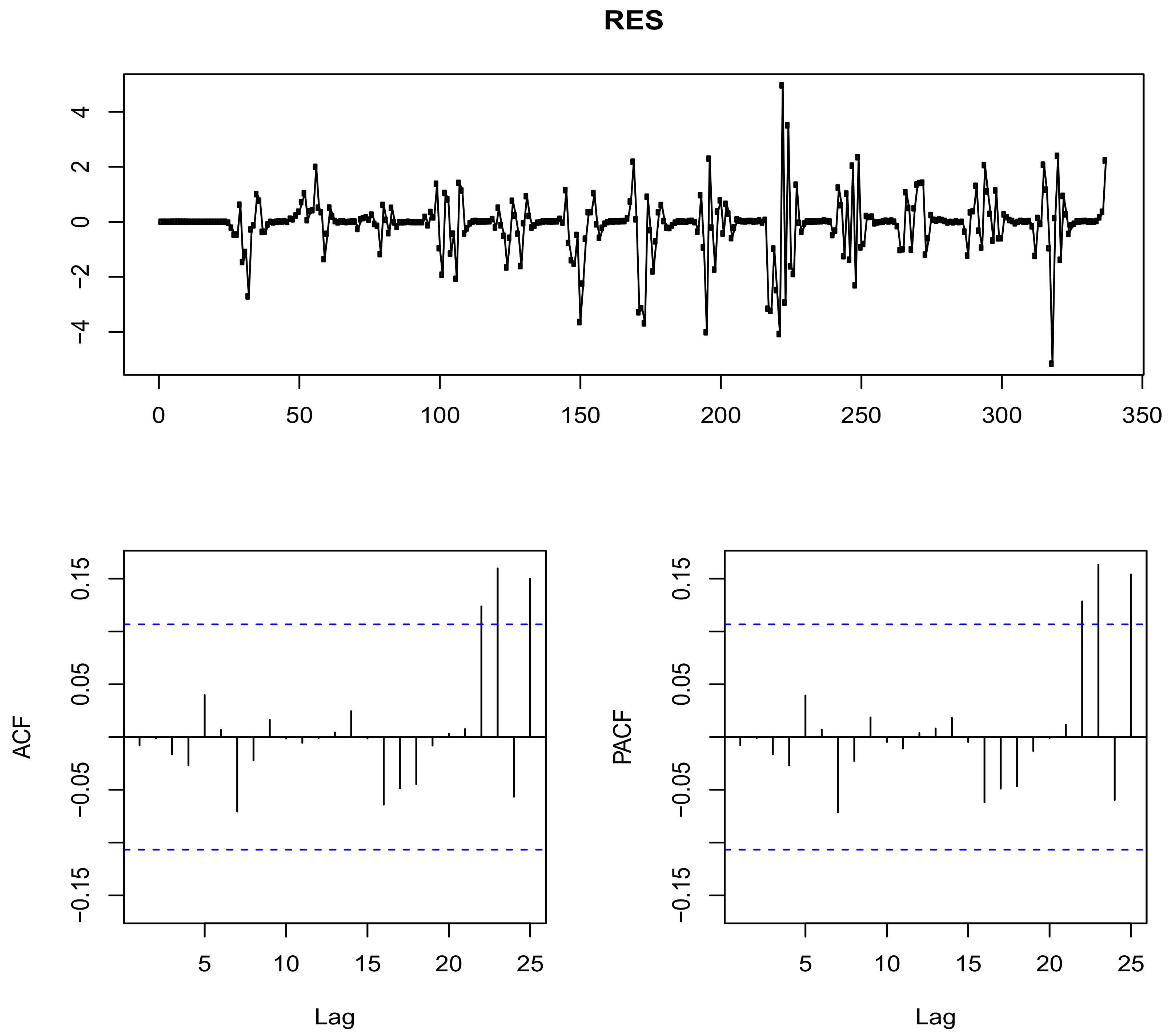
2.2.2. Residual Analysis

After fitting a model, it is important to determine whether all the necessary assumptions of the residuals are valid before performing inference because if there are any violations, the subsequent inferential procedures may be invalid resulting in faulty conclusions. One of the tests will be to check whether or not the residuals are autocorrelated. The residuals, ${\epsilon }_{t,\tau }$ are defined as the difference between the actual and the fitted values and are expressed as shown in Equation (12).

$${\epsilon }_{t,\tau }=y_{t,\tau }-{\widehat{y}}_{t,\tau },t=1,...,n,$$

(12)

where $y_{t,\tau }$ are the actual values of a response variable and ${\widehat{y}}_{t,\tau }$ are the estimated values of a response variable [17].

When fitting a model the autocorrelation of the residuals also has to be considered and accounted for. When the original data is highly autocorrelated, the residuals have a high risk of being autocorrelated. Thus, autocorrelation has to be dealt with, however this can be done by adding more parameters in the fit. Reducing all autocorrelation by adding more parameters is quite hard. Therefore a SARIMA model can be added to the model. A formal test for autocorrelation can be summarized as follows [29,30]:

• Estimate the parameters;
• Check if the response variables and predictors are stationary using the Kwiatkowski-Phillips-Schmidt-Shin (KPSS) unit root test;
• If not apply differencing until all variables become stationary;
• Extract residuals and use the Ljung Box-test to test for autocorrelation and if still autocorrelated, identify an appropriate SARIMA model by repeating the process until the desired results are achieved. The residuals are also tested for normality using the Shapiro-Wilk test.

2.3. Forecast Combination

Combining forecasts was first introduced by Reference [31]. It is particularly useful when one is uncertain about a situation, uncertain about which method is most accurate and when one wants to avoid large errors. It improves the forecast accuracy to the extent that the component contains useful and independent information.

2.3.1. Convex Combination

The loss functions play important roles in forecast combination in two ways. The first one is that they may serve as a key ingredient in combination formulas and the second one is that they are used to define performance evaluation criteria. In the first direction the use of loss functions is found in many popular combination schemes such as regression based combination and many adaptive forecast combination methods. Let $y_{t,\tau }$ be hourly GHI and let there be K methods used to predict the next m observations of $y_{t,\tau }$, that is, m is the total number of forecasts. The combined forecasts, $z_{t,\tau }$ are then given by Equation (13) [32,33]:

$$z_{t,\tau }=\sum _{k=1}^K{w}_{t,k,\tau }{\widehat{y}}_{t,k,\tau }+{\epsilon }_{t,\tau },\tau \in (0,1),t=1,...,m,$$

(13)

where $w_{t,k,\tau }$ is the weight assigned to the forecast ${\widehat{y}}_{t,k,\tau }$ and ${\epsilon }_{t,\tau }$ denotes the error term.

2.3.2. Quantile Regression Averaging

Quantile regression averaging (QRA) was first introduced by Reference [34] as a new approach to compute the prediction intervals. It can be viewed as an extension of combining forecasts. It involves applying QR to the forecasts of a small number of individual forecasting models. This approach treats the individual forecasts as the independent variables and the corresponding observation as the dependent variable (GHI). Let $y_{t,\tau }$ be hourly GHI as discussed in Section 2.1, then combined forecasts will be given by Equation (14).

$${\widehat{y}}_{t,\tau }^{\mathrm{QRA}}={\omega }_{0,\tau }+\sum _{k=1}^K{\omega }_{k,\tau }{\widehat{y}}_{t,k,\tau }+{\epsilon }_{t,\tau },\tau \in (0,1),t=1,...,m,$$

(14)

where ${\widehat{y}}_{t,k,\tau }$ represents forecasts from method k, ${\widehat{y}}_{t,\tau }^{\mathrm{QRA}}$ is the combined forecasts and ${\epsilon }_{t,\tau }$ is the error term.

2.4. Error Measures for Probabilistic Forecasting and Evaluation of Methods

In order to compare the probabilistic forecasts from the different models, scoring rules will be used. A penalty score denoted by $S(y,F)$ is assigned by a scoring rule to the probabilistic forecast, where y is the observation used in evaluating the forecast and F denotes the forecast distribution [35]. In this paper we use three error measures, that is the continuous rank probability score (CRPS), Dawid-Sebastiani score (DSS) and the pinball loss function (PLF).

2.4.1. Continuous Rank Probability Score

The CRPS measures the distance between the predicted and the observed cumulative density functions (CDFs) of scalar variables [35]. The CRPS is given as:

$$\begin{array}{c}\hfill CRPS(y,F)={\int }_0^1{QS}_{\tau }\left(F^{-1}\left(\tau \right),y\right)d\tau ,\end{array}$$

(15)

where F is the forecast distribution and ${QS}_{\tau }$ is the quantile score given as:

$$\begin{array}{c}\hfill {QS}_{\tau }\left(F^{-1}\left(\tau \right),y\right)=2\left(\mathbf{I}\left[y\le F^{-1}\left(\tau \right)\right]-\tau \right)\left(F^{-1}\left(\tau \right)-y\right),\end{array}$$

(16)

where I is an indicator function.

2.4.2. Dawid-Sebastiani Score

For complex forecast distributions, the CRPS is normally difficult to compute [36]. An alternative to the CRPS is the DSS which is relatively easier to compute. The DSS is given in Equation (17) [36].

$$\begin{array}{c}\hfill \mathrm{D}\mathrm{S}\mathrm{S}(y,F)=\frac{{(y-{\mu }_F)}^2}{\left({\sigma }_F^2\right)}+2\mathrm{l}\mathrm{o}\mathrm{g}\left({\sigma }_F\right),\end{array}$$

(17)

where F is the forecast distribution, with ${\mu }_F$ and ${\sigma }_F$ representing the mean and standard deviation, respectively.

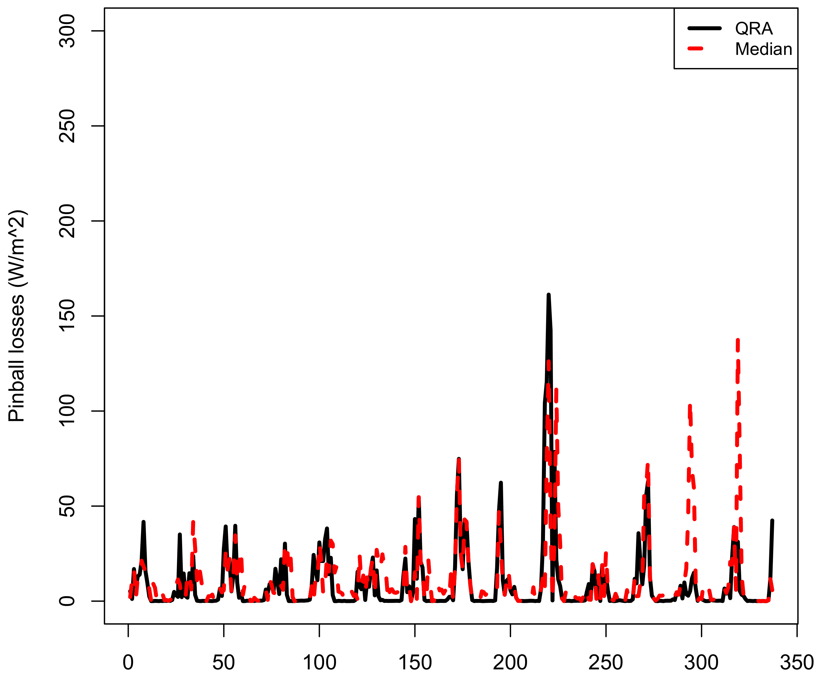
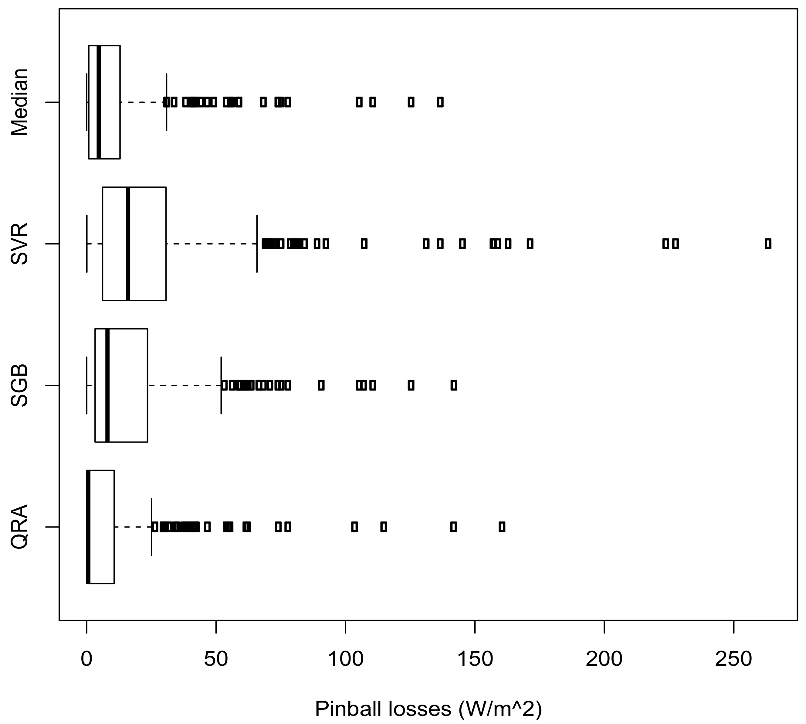
2.4.3. Pinball Loss Function

The pinball loss function is relatively easy to use and is given as:

$$L(q_{\tau },y_t)=\left\{\begin{array}{cc}\tau (y_t-q_{\tau }),\hfill & \mathrm{if}{y}_t>q_{\tau },\hfill \\ (1-\tau )(q_{\tau }-y_t),\hfill & \mathrm{if}{y}_t\le q_{\tau },\hfill \end{array}\right.$$

(18)

where $q_{\tau }$ is the quantile forecast and $y_t$ is the observed value of GHI.

2.5. Prediction Intervals

Providing prediction intervals of the future forecasts helps decision makers in power utility companies in assessing future uncertainty of the power supply [2,3]. We discuss briefly in the following sections, prediction interval widths and performance of estimated prediction intervals.

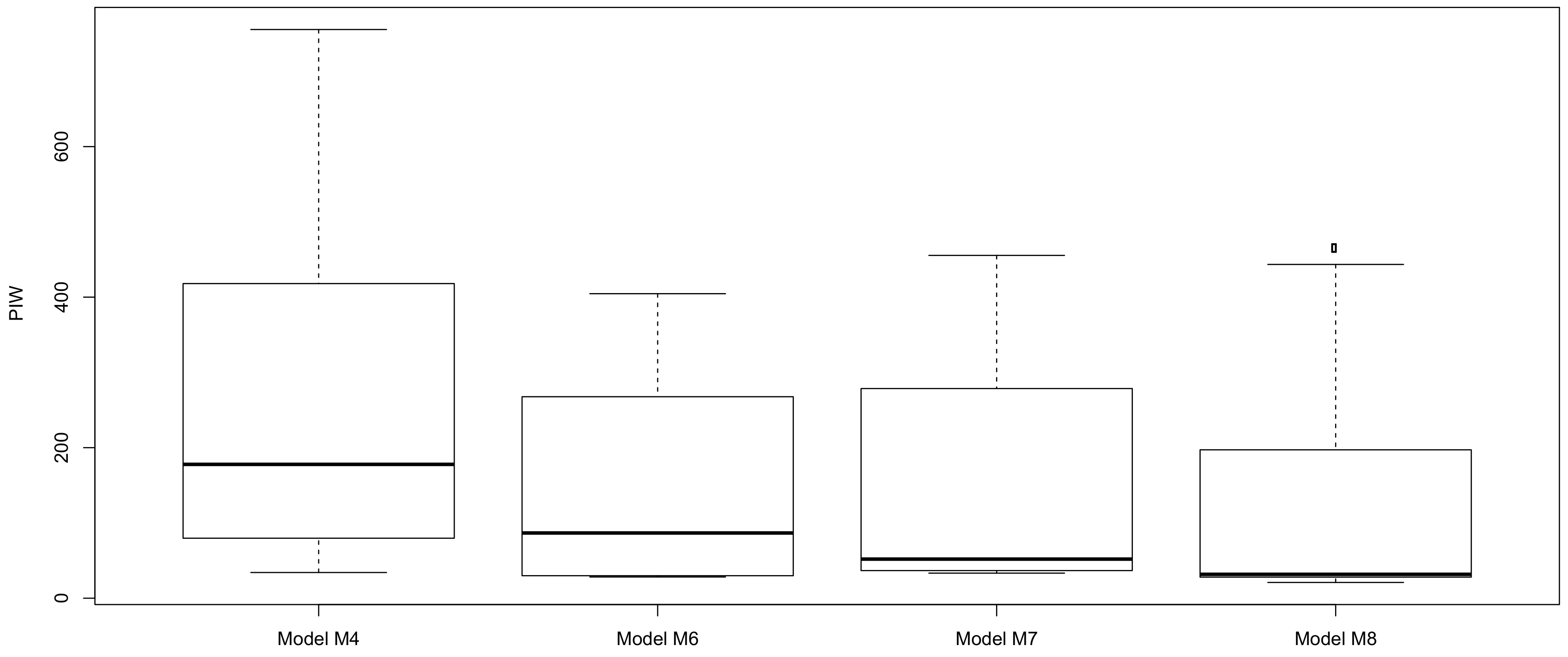
2.5.1. Prediction Intervals Widths

Prediction interval width (PIW) is the difference of the estimated upper and lower limit values. Generally it is given by the following Equation (19) [37]:

$${\mathrm{P}\mathrm{I}\mathrm{W}}_t=U_t-L_{t}t=1,...,h,$$

(19)

where $U_t$ and $L_t$ is the upper and lower limit. The PI normalised Average Width (PINAW) and PI Coverage Probability (PICP), respectively are used to evaluate the performance of prediction intervals (PIs). The PINAW describes the width of the PIs and the PICP evaluate the reliability of the PIs and are given by Equations (20) and (21), respectively [37]:

$$\mathrm{P}\mathrm{I}\mathrm{N}\mathrm{A}\mathrm{W}=\frac{1}{h}\sum _{t=1}^h\frac{PI{W}_t}{y_{max}-y_{min}},$$

(20)

$$\mathrm{P}\mathrm{I}\mathrm{C}\mathrm{P}=\frac{1}{h}\sum _{t=1}^h{I}_t{I}_t=\left\{\begin{array}{c}1if{y}_tϵ(L_t,U_t)\hfill \\ 0otherwise\hfill \end{array}\right.,$$

(21)

where $y_{min}$ and $y_{max}$ represent the minimum and the maximum values of PIW respectively. For the PIs to be valid, the PICP value has to be greater than or equal to the predetermined confidence level. The deviation degree from the actual value to the PIs is described by the PI normalised Average Deviation (PINAD). The PINAD is defined as [37]:

$$\mathrm{P}\mathrm{I}\mathrm{N}\mathrm{A}\mathrm{D}=\frac{1}{h}\sum _{t=1}^h\frac{d_t}{y_{max}-y_{min}}{d}_t=\left\{\begin{array}{c}{L}_t-y_{t}if{y}_t<L_t\hfill \\ 0if{L}_t\le y_t\le U_t\hfill \\ y_t-U_{t}if{y}_t>U_t\hfill \end{array}\right..$$

(22)

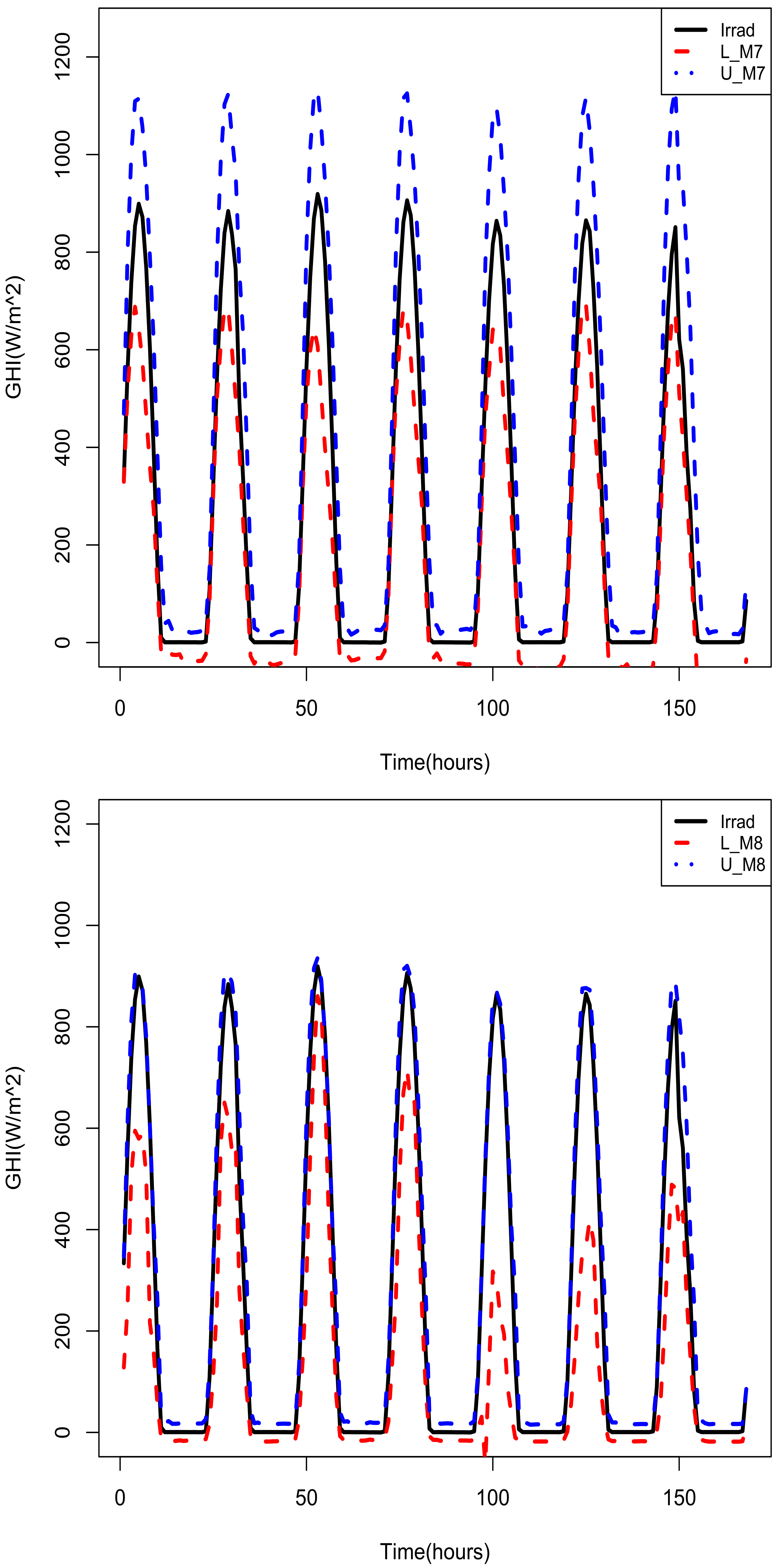
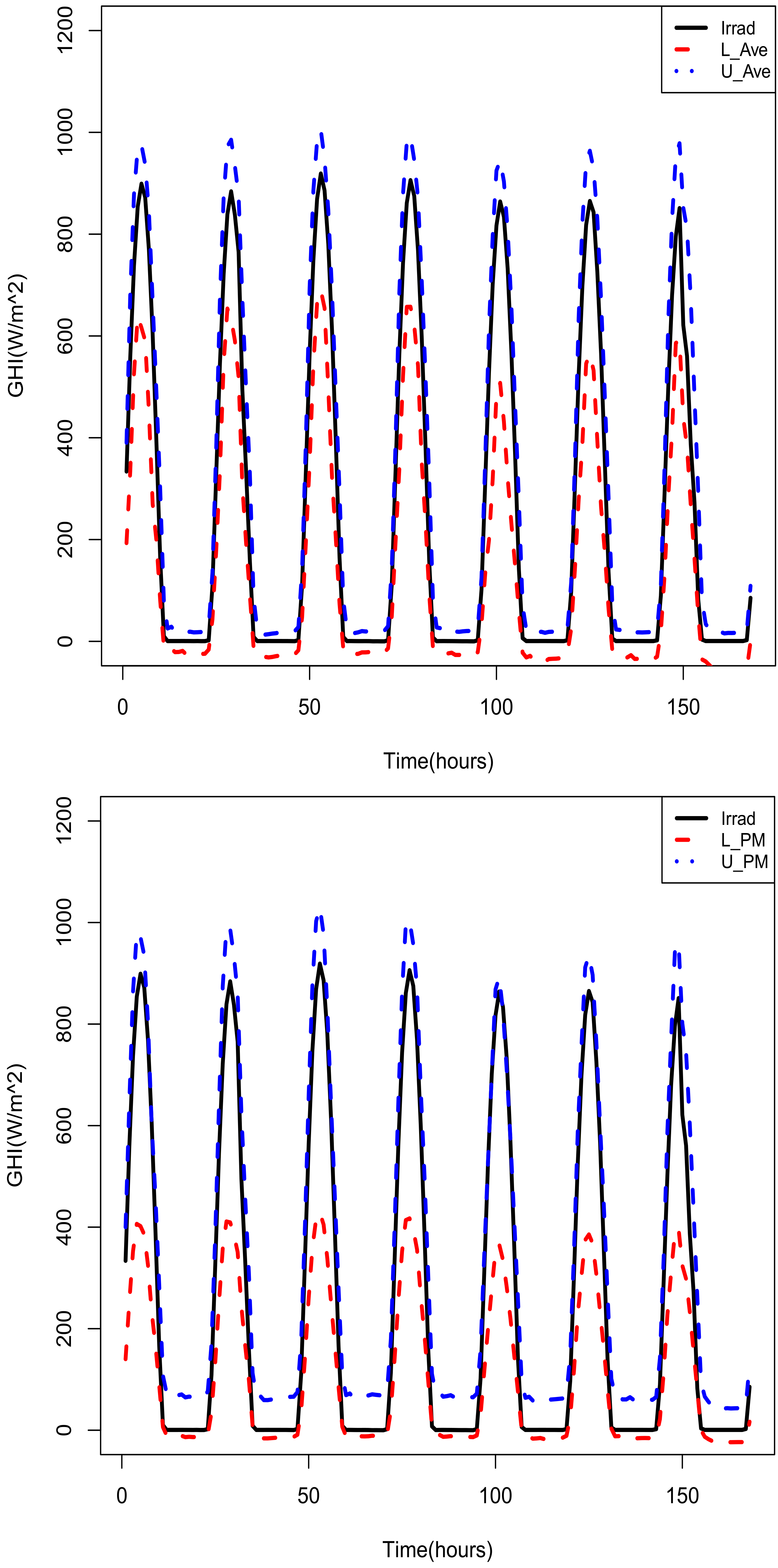
2.5.2. Performance of Estimated Prediction Intervals

Research has shown that combining point forecasts can improve the accuracy of the forecasts ([31,32]). This is then extended to combining prediction limits of the combined forecasts. In this section we present prediction interval combinations from the models M6, M7 and M8 and compare the combined intervals from the intervals of the individual models.

Let $[L_k,U_k],k=1,...,K$ be the $100(1-\alpha )\%$ prediction intervals given by K forecasting methods (the K methods discussed in Section 2.3.1). Let $[L_C,U_C]$ denote the $100(1-\alpha )\%$ combined prediction intervals using the interval combining method C [3]. In this paper we are going to use the simple average (Av), median (Md) and the probability averaging of endpoints and simple averaging midpoints (PM) as discussed in Reference [3].

Simple Average

This method takes the simple arithmetic means of the prediction limits given as $L_{Av}=\frac{1}{K}{\sum }_{k=1}^K{L}_k$ and $U_{Av}=\frac{1}{K}{\sum }_{k=1}^K{U}_k$. This approach is fairly simple and is known to produce intervals which are robust [3].

Median Method

The median method is also fairly easy to use and is not sensitive to outliers. It is given as [3]: $L_{Md}=median(L_1,...,L_K)$ and $U_{Md}=median(U_1,...,U_K)$.

Probability Averaging of Endpoints and Simple Averaging of Midpoints

The probability averaging of endpoints and simple averaging of midpoints (PM) combines simple averaging with probability averaging [3]. It is assumed that the prediction limit points are from a symmetric distribution (normal distribution). This results in finding the centre of the combined interval limits as $C=\frac{1}{2K}{\sum }_{k=1}^K(L_k+U_k)=\frac{1}{2}(\overline{L}+\overline{U})$. The lower ($L_{PM}$) and upper ($U_{PM}$) limits are then chosen such that $\frac{1}{K}{\sum }_{k=1}^K{F}_k\left(L_{PM}\right)=\frac{\alpha }{2}$ and $\frac{1}{K}{\sum }_{k=1}^K{F}_k\left(U_{PM}\right)=1-\frac{\alpha }{2}$ with $F_k$ denoting the distribution function of a normal distribution [3].

2.6. Benchmark Models

2.6.1. Stochastic Gradient Boosting

Gradient boosting (GB) is a machine learning technique which fits an additive model in a stage-wise way. The additive model can take the form given in Equation (23) [38].

$$f\left(x\right)=\sum _{m=1}^M{\beta }_{m}b(x;{\gamma }_m),$$

(23)

where $b(x;{\gamma }_m)\in \mathbb{R}$ are functions of x which are characterised by the expansion parameters ${\gamma }_m$, ${\beta }_m$. The parameters ${\beta }_m$ and ${\gamma }_m$ are fitted in a stage-wise way, a process which slows down over-fitting [38]. Stochastic gradient boosting (SGB) is a modification of GB in which a random sample of the training data set is taken without replacement. A more detailed discussion of this is found in Reference [39].

2.6.2. Support Vector Regression

Support vector regression (SVR) is based on support vector machines (SVM) and uses different kernel functions which map low dimensional data to high dimensional space. Introduced by Reference [40], SVR seeks to estimate a regression function of the form given in Equation (24).

$$\begin{array}{c}\hfill f\left(x\right)=x^{T}w+b,\end{array}$$

(24)

where b is a scalar and $\omega$ is a vector of weights. Equation (24) can be reformulated as a quadratic programming problem (QPP) by introducing an $\epsilon$-insensitive loss function as given in Equation (25) [40].

$$\begin{array}{c}\hfill \underset{(\omega ,b,{\xi }_1,{\xi }_2)}{min}\frac{1}{2}{\omega }^T\omega +C(e^T{\xi }_1+e^T{\xi }_2)\\ \hfill s.t.y_i-x_i^T\omega -b\le \epsilon +{\xi }_1\\ \hfill x_i^T\omega +b-y_i\le \epsilon +{\xi }_2\\ \hfill and{\xi }_{1i},{\xi }_{2i}\ge 0,i=1,...,m,\end{array}$$

(25)

where $C>0,\epsilon >0$ are input parameters, ${\xi }_1={({\xi }_{11},...,{\xi }_{1m})}^T$ and ${\xi }_2=({\xi }_{21},...,{\xi }_{2m})$ are slack variables. The QPP in Equation (24) can be reformulated using Lagrange multipliers. Only the non-zero Lagrange multipliers are important in the prediction of the regression function. A kernel function, $k(.,.)$ is used in cases where there are non-linear regressors. When a non-linear regressor is used, the regression function in Equation (24) is then written as:

$$\begin{array}{c}\hfill f\left(x\right)=\sum _{i=1}^m({\lambda }_{1i}-{\lambda }_{2i})k(x,x_i)+b,\end{array}$$

(26)

where ${\lambda }_{1i}$ and ${\lambda }_{2i}$ are Lagrange multipliers. The Lagrange formulation of the non-linear case is given as:

$$\begin{array}{c}\hfill \underset{({\lambda }_1,{\lambda }_2)}{min}\frac{1}{2}\sum _{i,j=1}^m{({\lambda }_{1i}-{\lambda }_{2i})}^{T}k(x_i,x_j)({\lambda }_{1i}-{\lambda }_{2i})+\epsilon \sum _{i=1}^m({\lambda }_{1i}-{\lambda }_{2i})-\sum _{i=1}^m{y}_i({\lambda }_{1i}-{\lambda }_{2i})\\ \hfill s.t.\sum _{i=1}^m({\lambda }_{1i}-{\lambda }_{2i})=0\\ \hfill and{\lambda }_1\ge 0,{\lambda }_2\le Ce.\end{array}$$

(27)

3. Empirical Results and Discussion

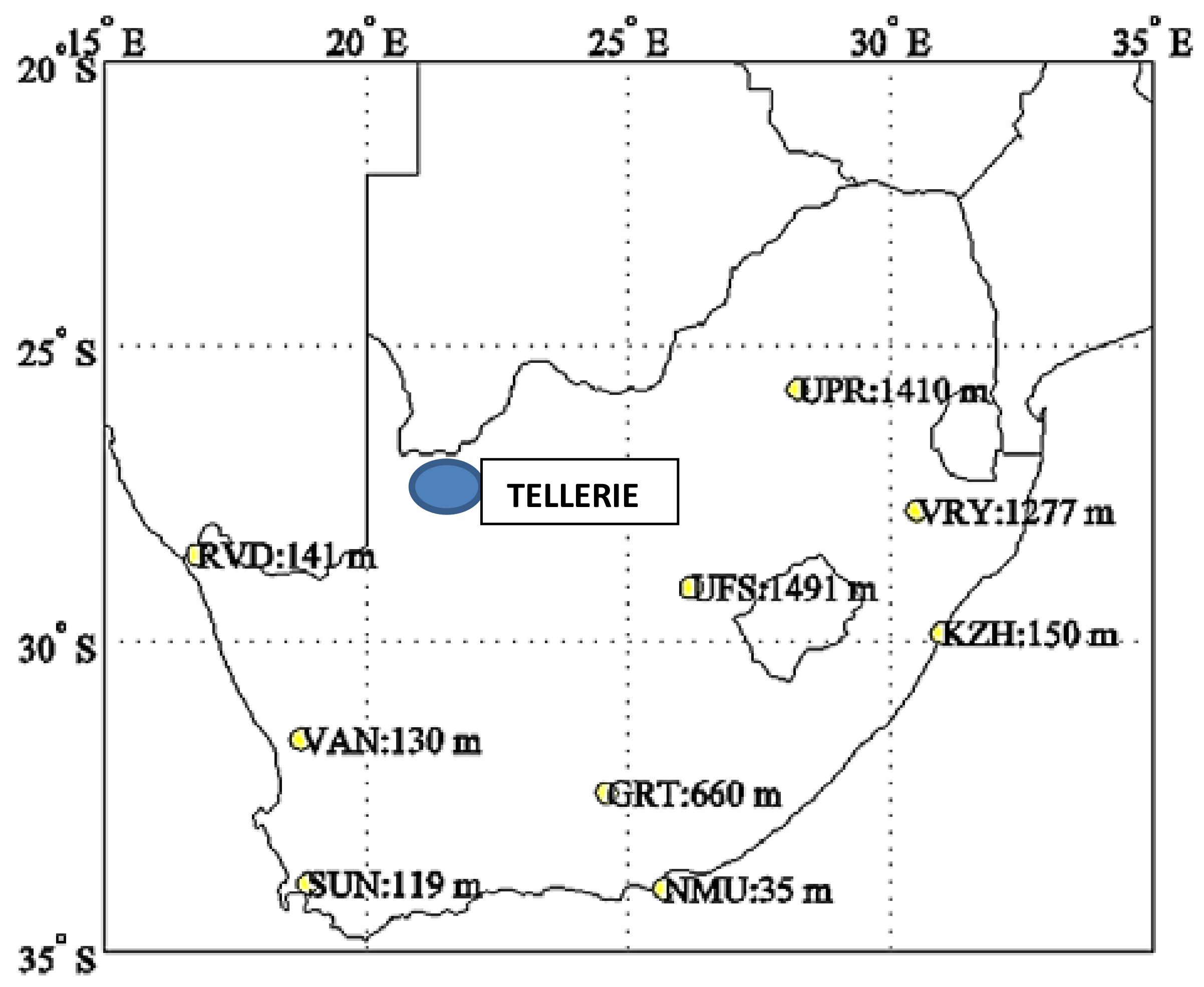
3.1. Data Source

The data used in this study is hourly averaged GHI (average W/m${}^2$) measured by Eskom (www.eskom.co.za), at site Tellerie in Northern Cape, South Africa for the period August 2009 to April 2010 giving a sample size of $n=5698$ observations. The target variable is the GHI (average W/m${}^2$). The covariates used in this study are (these were the only available covariates on the Eskom website): Relative humidity (RH_Avg), Rain fall (RN), Wind speed (WS_ms_S_WVT), Air temperature (AirTC_Avg), Barometric pressure (BP_mbar_Avg) and Wind direction (WindDir_D1_WVT).

In addition to the covariates given above, a factor variable (Hour (Hr)), Hour = 1, Hour = 2,..., Hour = 24; a non-linear trend (noltrend) and lagged GHI (Lag1 and Lag2) variables are added in order to model the trend in the time series data and also to help in reducing the autocorrelation, respectively. A non-linear trend is obtained by fitting a penalised cubic smoothing spline to the response variable (GHI). The penalised cubic smoothing spline function is given by Equation (28):

$$\mathrm{\Pi }\left(t\right)=\sum _{t=1}^n{(y_t-f\left(t\right))}^2+\lambda \int f^{\prime \prime }{\left(t\right)}^{2}d\left(t\right),$$

(28)

where $\lambda$ is the smoothing parameter which is selected based on the generalised cross validation (GCV) criterion. Lag1 and Lag2 represent the lagged GHI of the first and second previous hours, therefore taking the lags reduced the sample size from 5700 to 5698.

The wind speed and wind direction are both measured at 9m levels. All the variables provided have an impact on the solar irradiance generated. There are many predictors of solar irradiance that are left out in this study such as surface pressure, total cloud cover, total precipitation and so forth. These variables were not available on the Eskom website. The exact location of Tellerie radiometric station is:

• Latitude: ${27}^{\circ }22.{505}^{\prime }$ S
• Longitude: ${21}^{\circ }17.{799}^{\prime }$ E

The map of South Africa showing the location of the Eskom solar measuring station Tellerie located in Northern Cape is presented in Figure 1.

Figure 1. Map of South Africa showing the location of the Eskom solar measuring station Tellerie located in Northern Cape [41].

The data for the period 28 August 2009 (00:00 hour) to 8 April 2010 (10:00 hour) is used for training ($n_1=5362$ observations), while the remaining data that is, 9 April 2010 (11:00 hrs) to 22 April 2010 (09:00 hrs) ($n_2=336$ observations) are used for testing. The training and testing data sets are used for all the models developed in this study.

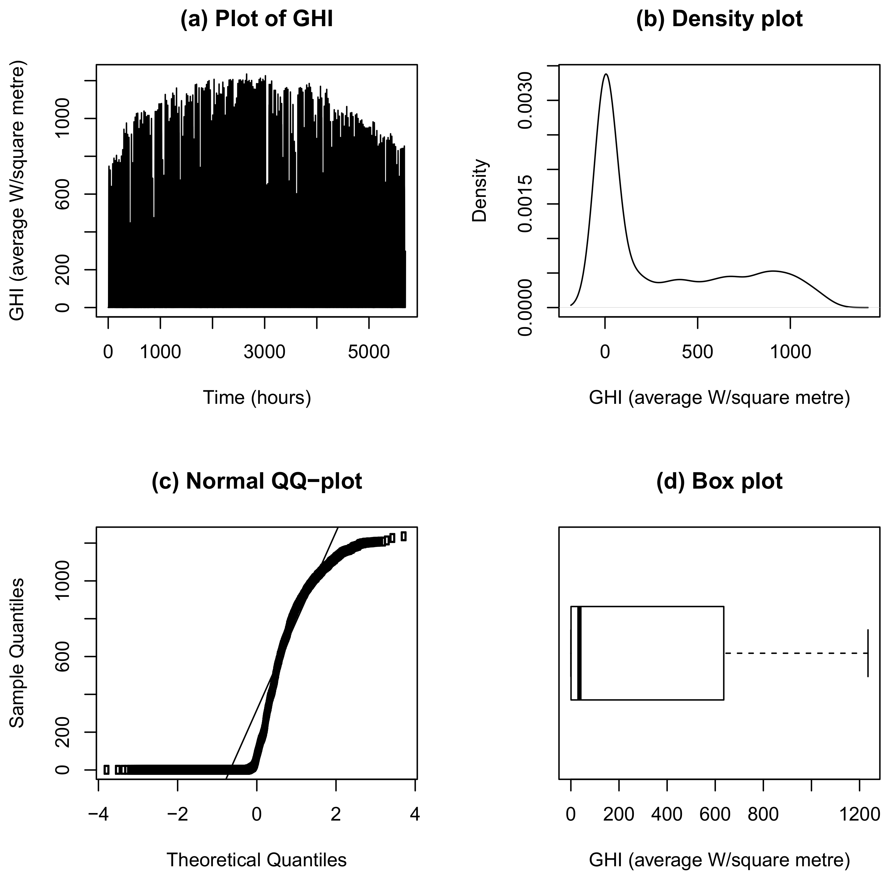
3.2. Exploratory Data Analysis

It is considered important to first do an exploratory data analysis of the historical data before setting up the forecasting models. The time series, density, box and normal Q-Q plots for the dependent variable (GHI (average W/m${}^2$)) are given in Figure 2 in the panels (a), (b), (c), (d), respectively. Plot (a) in Figure 2 displays GHI (average W/m${}^2$) in South Africa measured hourly from 2009–2010. It indicates that there is an upward trend from observation 1–3000, followed by a downward trend from observation 3000–5700. The density plot shown in panel (b) of Figure 2 the distribution of GHI is skewed to the right suggesting that it is not normally distributed. Plot (c) shows a non-linear relationship between the theoretical and sample quantiles of GHI suggesting that GHI data are not normally distributed as is also confirmed by the boxplot in panel (d).

Figure 2. Panel (a): Plot of global horizontal irradiance (GHI) (W/m${}^2$). Panel (b): Density plot of GHI. Panel (c): Normal Q-Q plot of GHI. Panel (d): Box plot of GHI.

Summary statistics of GHI showing a minimum GHI of 0 (average W/m${}^2$) and maximum GHI of 1235 (average W/m${}^2$) is given in Table 1. The skewness coefficient presented in Table 1 indicates that the distribution of GHI is skewed to the right. The mean and the median are not equal and the Jarque-Bera statistic is 854.21 with a p-value of 0.000 which confirms that the distribution is not normally distributed.

Table 1. Summary statistics of the GHI (average W/m${}^2$).

Min	1st Qu	Median	Mean	3rd Qu	Max	Skewness	Kurtosis	Jarque-Bera
0.000	0.64	34.84	305.91	635.20	1235.00	0.86	−0.79	854.21 (0.000)

3.3. Forecasting Results

3.3.1. Variable Selection Using Lasso Via Hierarchical Interactions

Variable selection using Lasso via hierarchical interactions is carried out and a summary of the results are presented in Table 2.

Table 2. Variables selected using Lasso via hierarchical interactions.

	Main Effect	RN	WS	WindDir	AirTC	RH	BP	HOUR	noltrend	Lag1	Lag2	Tight?
RN	−6.29	−4.62	0	0	0	0	0	0	0	0	−1.67
WS	4.04	0	0	0	0	0	4.04	0	0	0	0
WindDir	8.87	0	0	−1.14	0	0	4.29	−3.007	0.43	0	0	*
AirTC	169.62	0	0	0	43.81	−15.83	0.61	−106.10	0	0	0
RH	−49.30	0	0	0	−15.83	0.49	−4.21	28.77	0	0	0	*
BP	38.28	0	4.04	4.29	0.61	−4.21	0	0	0	0	8.26
HOUR	−97.36	0	0	−3.00	−106.10	28.77	0	−196.79	0	0	0	*
noltrend	0.43	0	0	0.43	0	0	0	0	0	0	0
Lag1	2.845	0	0	0	0	0	0	0	0	−2.85	0	*
Lag2	14.19	−1.67	0	0	0	0	8.26	0	0	0	0

The first column indicates the main effect, next columns indicate the non-zero interactions of the row predictor and the last column indicates whether hierarchy constraint is tight or not, 0 indicate that there is no interactions between the variables. The variables with interactions are RN and Lag2, WS and BP, WindDir and BP, WindDir and HOUR, WindDir and noltrend, AirTC and BP, AirTC and HOUR, AirTC and noltrend, RH and AirTC, RH and BP, RH and HOUR, BP and Lag2.

3.3.2. Variable Importance

Table 3 shows the relative contribution of the variables used in this study. It can be seen that the variable “hour” has the highest relative importance, meaning that the hour of the day is very important for GHI, followed by air temperature. The selected variables are then used in all the developed models in this study including the benchmark models.

Table 3. Variable importance.

Variable	Relative Influence
hour	40.458
AirTC	30.769
Lag2	11.019
RN*Lag2	10.884
noltrend	2.535
BP*Lag2	1.867
Lag1	0.594
AirTC*hour	0.430
WindDir*hour	0.359
RH	0.285
RH*AirTC	0.224
RN	0.164
WS*BP	0.146
WindDir*BP	0.127
WindDir*noltrend	0.071
WindDir	0.036
BP	0.021
WS	0.010

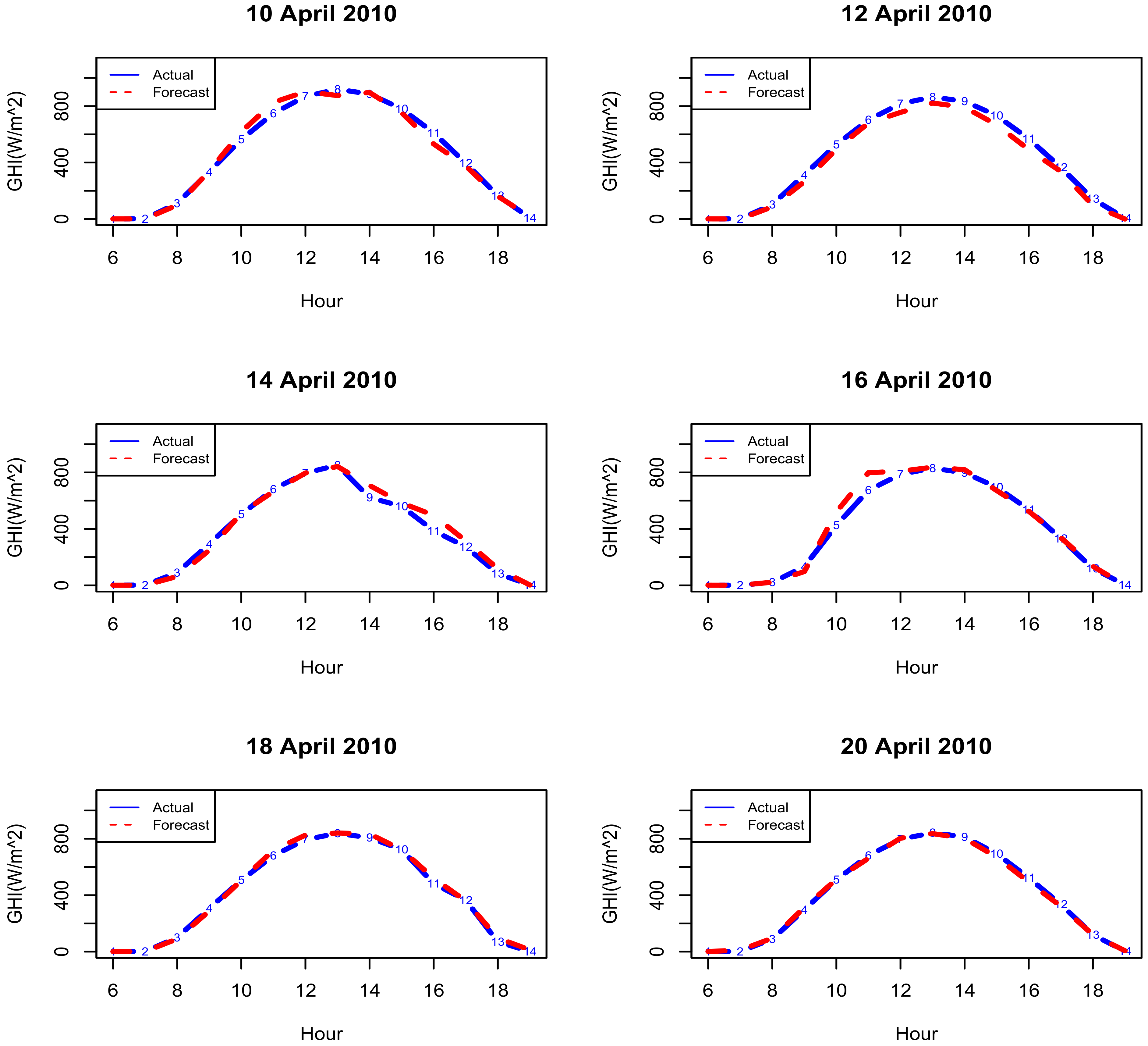
3.3.3. Partially Linear Additive Quantile Regression Models with and Without Interactions

PLAQR models are considered so as to relax the assumption that there is a linear relationship between the covariates in QR. This is done for $\tau =0.5$ using R-package “plaqr” developed by Reference [42]. The PLAQR models containing a set of predictors which have a linear relationship with the response variable, solar irradiance and a set of predictors which have unknown non-linear relationship with solar irradiance is given by the Equations (29) and (30), respectively:

$$\begin{array}{c}\hfill y_{t1}={\beta }_0+{\beta }_1\mathrm{R}\mathrm{H}+{\beta }_2\mathrm{B}\mathrm{P}+bs\left(\mathrm{R}\mathrm{N}\right)+bs\left(\mathrm{W}\mathrm{S}\right)+bs\left(\mathrm{W}\mathrm{i}\mathrm{n}\mathrm{d}\mathrm{D}\mathrm{i}\mathrm{r}\right)+bs\left(\mathrm{A}\mathrm{i}\mathrm{r}\mathrm{T}\mathrm{C}\right)+bs\left(\mathrm{H}\mathrm{r}\right)\\ \hfill +bs\left(\mathrm{n}\mathrm{o}\mathrm{l}\mathrm{t}\mathrm{r}\mathrm{e}\mathrm{n}\mathrm{d}\right)+bs\left(\mathrm{l}\mathrm{a}\mathrm{g}1\right)+bs\left(\mathrm{l}\mathrm{a}\mathrm{g}2\right)+{\epsilon }_{t1}\end{array}$$

(29)

and

$$\begin{array}{c}\hfill y_{t2}={\beta }_0+{\beta }_1\mathrm{R}\mathrm{N}+{\beta }_2\mathrm{R}\mathrm{H}+{\beta }_3\mathrm{B}\mathrm{P}+{\beta }_4\mathrm{n}\mathrm{o}\mathrm{l}\mathrm{t}\mathrm{r}\mathrm{e}\mathrm{n}\mathrm{d}+{\beta }_5\mathrm{L}\mathrm{a}\mathrm{g}1+{\beta }_6\mathrm{L}\mathrm{a}\mathrm{g}2+{\beta }_6\left(\mathrm{W}\mathrm{i}\mathrm{n}\mathrm{d}\mathrm{D}\mathrm{i}\mathrm{r},\mathrm{H}\mathrm{r}\right)\\ \hfill +{\beta }_7\left(\mathrm{W}\mathrm{i}\mathrm{n}\mathrm{d}\mathrm{D}\mathrm{i}\mathrm{r},\mathrm{n}\mathrm{o}\mathrm{l}\mathrm{t}\mathrm{r}\mathrm{e}\mathrm{n}\mathrm{d}\right)+{\beta }_8\left(\mathrm{R}\mathrm{H},\mathrm{A}\mathrm{i}\mathrm{r}\mathrm{T}\mathrm{C}\right)+bs\left(\mathrm{W}\mathrm{S}\right)+bs\left(\mathrm{W}\mathrm{i}\mathrm{n}\mathrm{d}\mathrm{D}\mathrm{i}\mathrm{r}\right)+bs\left(\mathrm{A}\mathrm{i}\mathrm{r}\mathrm{T}\mathrm{C}\right)\\ \hfill +bs\left(\mathrm{H}\mathrm{r}\right)+bs\left(\mathrm{R}\mathrm{N},\mathrm{l}\mathrm{a}\mathrm{g}2\right)+bs\left(\mathrm{W}\mathrm{S},\mathrm{B}\mathrm{P}\right)+bs\left(\mathrm{W}\mathrm{i}\mathrm{n}\mathrm{d}\mathrm{D}\mathrm{i}\mathrm{r},\mathrm{B}\mathrm{P}\right)\\ \hfill +bs\left(\mathrm{A}\mathrm{i}\mathrm{r}\mathrm{T}\mathrm{C},\mathrm{B}\mathrm{P}\right)+bs\left(\mathrm{A}\mathrm{i}\mathrm{r}\mathrm{T}\mathrm{C},\mathrm{H}\mathrm{r}\right)+bs\left(\mathrm{B}\mathrm{P},\mathrm{l}\mathrm{a}\mathrm{g}2\right)+{\epsilon }_{t2}\end{array}$$

(30)

where “$bs$” is a B-spline. The models are split into two, one with interactions (presented by $y_{t2}$) and the other without the interactions (presented by $y_{t1}$). The interactions presented in the above equations were found after doing variable selection using the Lasso via hierarchical interactions and the variables selected are RN and Lag2, WS and BP, WindDir and BP, WindDir and Hr, WindDir and noltrend, AirTC and BP, AirTC and Hr, AirTC and noltrend, RH and AirTC, RH and BP, RH and HOUR, BP and Lag2. After fitting the PLAQR models an autocorrelations test for the residuals was carried out.

The models considered in this study are: M1(GAM without interactions), M2 (GAM with interactions), M3(PLAQR model without interactions), M4(PLAQR model with interactions), M5(convex combination of models M1-M4), M6(GAM averaging), M7(convex averaging) and M8(quantile regression averaging). We present in the next paragraph a discussion of the results of the PLAQR models.

In order to reduce the autocorrelations for the PLAQR model without interactions, the SARIMA(4,1,4)(2,0,5)${}_s$ model is fitted to the residuals. This is followed by testing for autocorrelations using Ljung Box-test and find the p-value to be 0.3974 ($p>0.05$). For the PLAQR model with the pairwise interactions the SARIMA(4,1,4)(2,0,3)${}_s$ is then tested and a p-value of 0.2809 ($p>0.05$) is obtained. The best model is selected using AIC, BIC and the AdjR${}^2$. The better fitting model is the one with the minimum value of AIC, BIC and the maximum value of AdjR${}^2$ compared to the other models. Table 4 suggests that the model with the pairwise interactions (model M4) is considered to be the better model with the AdjR${}^2$ value of 0.957, AIC of 60,056.53 and BIC of 60,744.76.

Table 4. Model selection for partially linear additive quantile regression model (PLAQR) with and without interactions.

Models	AdjR${}^2$	AIC	BIC
PLAQR (M3)	0.947	61,191.64	60,748.55
PLAQR (M4)	0.954	60,744.76	60,056.53

The “opera” R-package developed by Reference [9] Gaillard and Goude 2015 is used to combine the forecasts. This is done in order to improve the accuracy measures obtained from these models. The convex combination of the models is done using an algorithm based on the pinball loss. The weights assigned to the forecasts for model M3 and model M4 are found to be $6.13\times {10}^{-21}$ and 1 respectively. Based on the pinball loss, model M4 (FQGAMI) is considered to be a better model since the weight assigned to it is 1. Therefore forecast combination is not necessary. Based on the pinball loss function the average loss suffered by the PLAQR model with pairwise interactions (model M4 (FQGAMI) in Figure 3) is smaller than that of the PLAQR without pairwise interactions (FQGAM in Figure 3).

Figure 3. Average loss based on pinball loss suffered by the developed models.

The combination of forecasts was then extended to QRA (Model M8) and is given by Equation (31):

$$y_{t,\tau \left(\mathrm{Q}\mathrm{R}\mathrm{A}\right)}={\beta }_{0,\tau }+{\beta }_1\mathrm{P}\mathrm{L}\mathrm{A}\mathrm{Q}\mathrm{R}+{\beta }_{2,\tau }\mathrm{P}\mathrm{L}\mathrm{A}\mathrm{Q}\mathrm{R}\mathrm{I}+{\epsilon }_{t,\tau },$$

(31)

where PLAQRI and PLAQR are the PLAQR with and without interactions. The Ljung BOX-test is applied to the residuals from the fitted QRA giving a Ljung Box-test statistic of 2320.2, with the p-value less than $2.2\times {10}^{-16}$. Since the p-value for the test statistic regarding the QRA is less than 0.05 it is concluded that the solar irradiance data has significant autocorrelation. In order to reduce the autocorrelation, SARIMA(3,0,2)(1,1,1)${}_s$ is fitted to the residuals resulting in a p-value of 0.9847 which is greater than 0.05. Therefore it is concluded that the data contain no autocorrelation up to lag 20 at the 5% level of significance as shown in Figure 4 bottom left panel. Visual inspection of the time series plot of the residuals in the top panel of Figure 4 indicates that the residuals are randomly scattered around mean zero.

Figure 4. Time series display of residuals from model M8 after correcting for autocorrelation.

Based on the boxplots of the prediction intervals shown in Figure 5, model M8 is the best fitting model as it has the narrowest PI compared to the other models, M4, M6 and M7.

Figure 5. Box plots of the rediction interval widths (PIWs) for models M4, M6, M7 and M8. PIW of model M8 appear to be the narrowest compared to the PIWs of the other models.

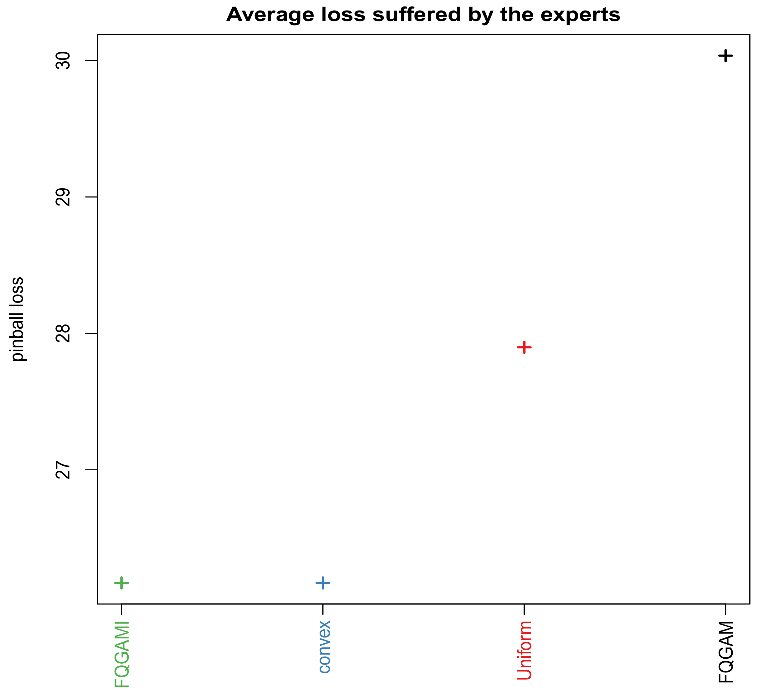
3.4. Quantile Regression Averaging and Comparative Analysis of the Models

3.4.1. Quantile Regression Averaging

QRA is an extension of combining probabilistic forecasts and is given by Equation (32):

$$y_{t,\tau \left(\mathrm{Q}\mathrm{R}\mathrm{A}\right)}={\beta }_{0,\tau }+{\beta }_1\mathrm{G}\mathrm{A}\mathrm{M}\mathrm{Q}\mathrm{R}\mathrm{A}+{\beta }_{2,\tau }\mathrm{P}\mathrm{L}\mathrm{A}\mathrm{Q}\mathrm{R}\mathrm{A}+{\beta }_{3,\tau }\mathrm{C}\mathrm{O}\mathrm{N}\mathrm{V}\mathrm{E}\mathrm{Q}\mathrm{R}\mathrm{A}+{\epsilon }_{t,\tau },$$

(32)

where GAMQRA, PLAQRA and CONVEXQRA are the regressed GAM, PLAQR and CONVEX forecasts, in this case taken as predictors of solar irradiance.

3.4.2. Comparative Analysis of the Models

A summary statistics of the residuals of the models is presented in Table 5. The models were then compared using using prediction intervals. A summary of PICP, PINAW and PINAD is presented in Table 6. From Table 6 the PINAW of model M8 is the lowest compared to those of models M6 and M7. The performance of the models against the best models which is model M8 is then calculated. The percentage improvement of M8 over M6 and M7 are found to be 8.49% and 13.87% respectively.

Table 5. Summary statistics of the residuals of the models.

Summary Statistics of Residuals
	Model M4	Model M6	Model M7	Model M8
Standard deviation	79.53	0.67	48.85	41.14
Mean	−25.12	−0.56	−6.56	−4.50
Median	4.49	−0.13	−0.10	−0.11
1st Quartile	−66.21	−1.04	−0.70	−0.94
3rd Quartile	26.23	−0.05	1.69	1.57
Skewness	−2.34	−1.34	−4.04	−3.45
Kurtosis	7.89	1.61	24.46	21.25
Under and over Predictions
Mean under predicted	0.53	0.43	0.43	0.42
Mean Over predicted	0.47	0.57	0.57	0.58
Under prediction	179	144	145	141
Over prediction	158	193	192	196

Table 6. Comparison of the best models using the PI Coverage Probability (PICP), PI normalised Average Width (PINAW) and PI normalised Average Deviation (PINAD) at 95% level of confidence.

Models	PICP	PINAW	PINAD	Mean PI
Model M6	98.52%	27.01%	0.08%	155.66
Model M7	98.81%	27.92%	0.09%	153.99
Model M8	98.82%	15.27%	0.05%	140.36

3.4.3. Comparative Analysis with the Benchmark Models

The median method discussed in Section 2.5.2 is also used in forecast combination as follows: Median forecast $=median(QRA,SVR,SGB)$. The median forecasts are then compared with the QRA forecasts and the forecasts from benchmark (machine learning) models as shown in Table 7. All the models in Table 7 have invalid PICPs, that is, they are less than $95\%$ except for model M8 (QRA). This therefore means that the PINAW and PINAD of the models with invalid PICPs would not have any meaning. However the Median forecasts have the smallest mean PI.

Table 7. Model comparisons.

Accuracy Measures	M8 (QRA)	SVR (Benchmark)	SGB (Benchmark)	MEdian Forecasts
CRPS	151.57	160.4182	167.55	158.83
Pinball loss	8.82	26.31	17.18	10.89
DSS	12.25	12.49	12.53	12.45
PICP	98.82%	84.57%	82.50%	89.91%
Mean PI	140.36	170.83	135.32	129.50

Table 7 also shows a summary of the accuracy measures for the models. Based on CRPS, DSS and pinball loss, model M8 is found to be the best compared to the median forecasts and the two benchmark models, SVR and SGB, respectively. M8 is then used for out of sample forecasting.

Figure 6 shows a plot of pinball losses (top panel) from the QRA and Median forecasts (8–22 April 2010, 337 forecasts) and box plots of pinball losses (bottom panel) from the QRA and Median forecasts. The box plots on Figure 6 suggests that the distribution of the pinball losses from the QRA model has the smallest variability and as such is the best fitting model compared to the benchmark models.

Figure 6. Top panel: Plot of pinball losses from the quantile regression averaging (QRA) and Median models in April 2010 (8–22 April 2010, 337 forecasts). Bottom panel: Box plots of pinball losses from the QRA, SGB, SVR and Median models in April 2010.

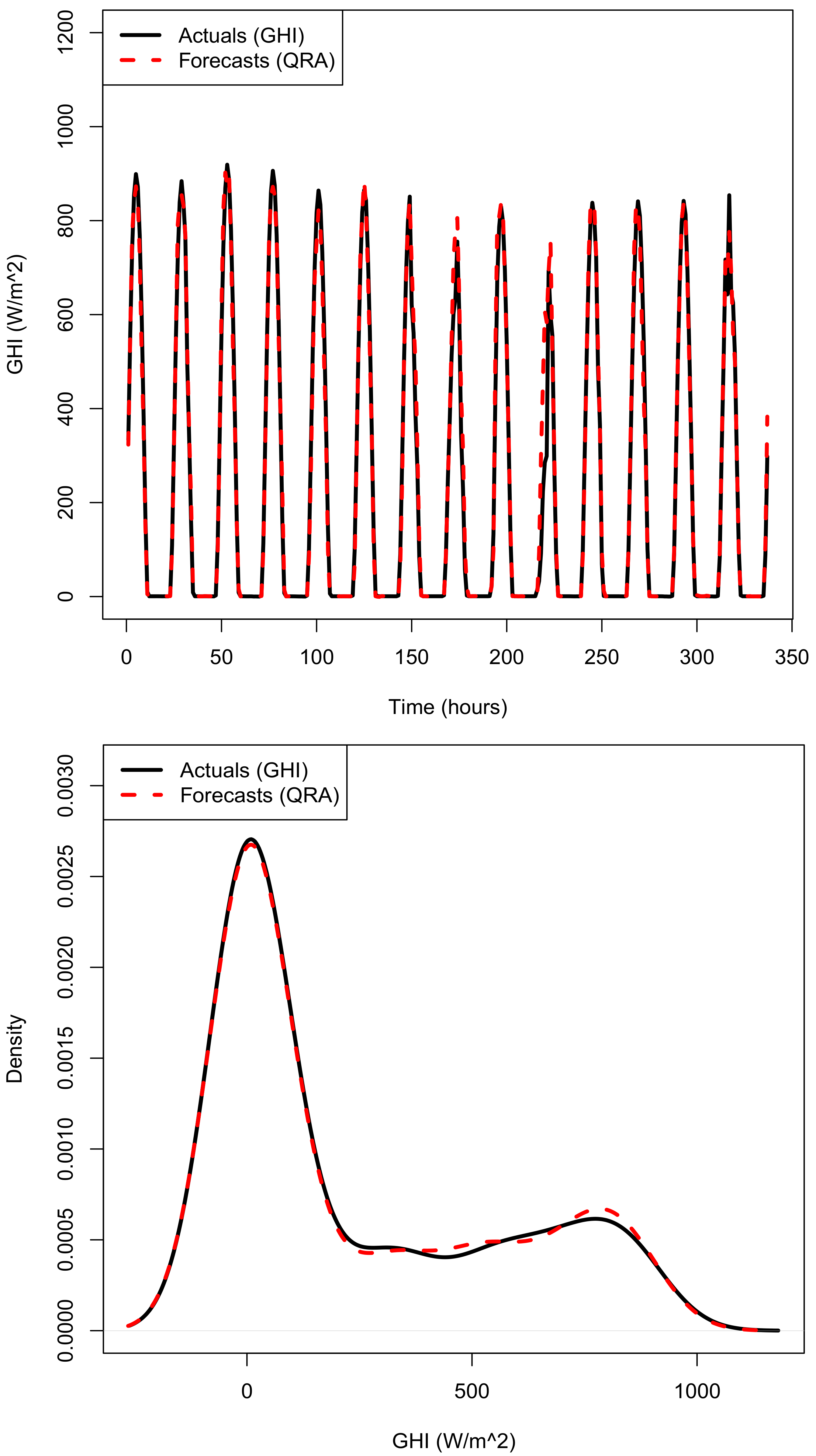
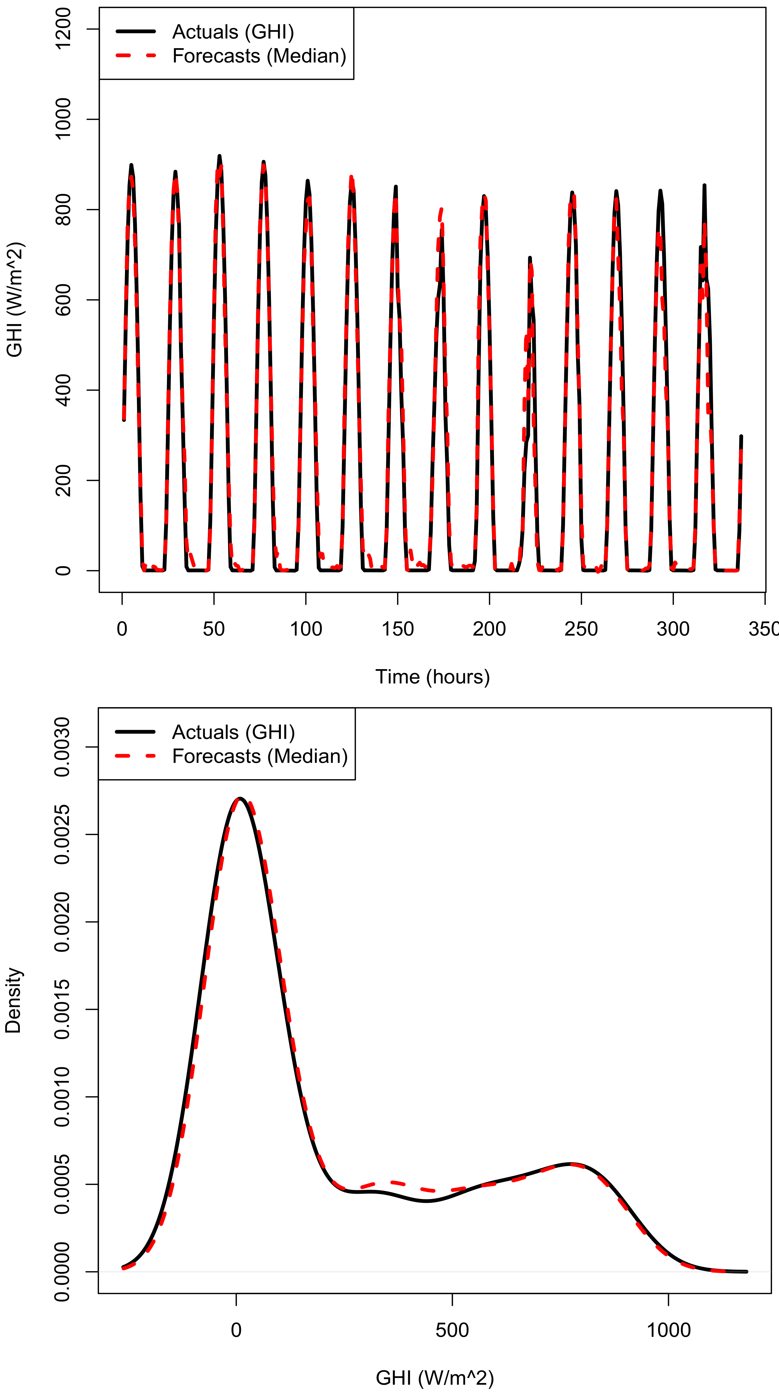
3.4.4. Combining Prediction Intervals and Out of Sample Forecasts

Overall the individual models are producing overconfident prediction intervals as shown by their hit rates which are well above the target of 0.95 (See Table 8, column 4). The prediction intervals from the individual models are then compared with the three simple interval combination methods discussed in Section 2.5.2. Results from Table 8 show that the PM is the best prediction limits combination method as it gives a hit rate of 0.955 which is very close to the target of 0.95.

Table 8. Comparison of prediction intervals.

Individual Models	Below Lower Limit	Above Upper Limit	Hit Rate
Model M6	4	3	0.979
Model M7	5	0	0.985
Model M8	3	1	0.988
Combinations
Simple average	3	0	0.991
Median	4	0	0.988
PM	7	8	0.955

The forecasts, dashed line from model M8 (QRA forecasts) follow the actual solar irradiance remarkably well (Figure 7 top panel). The forecast distribution of GHI, dashed lines (Bottom panel of Figure 7) follow very well the density of the actual GHI, solid line. Similar plots for the combined median forecasts are given in the appendix, Figure A1.

Figure 7. Top panel: Actual and predicted GHI in April 2010 (337 forecasts). Bottom panel: Actual and predicted density plots of GHI.

Figure 8 shows actual GHI, solid lines superimposed with forecasts, dashed lines (QRA forecasts) for some selected days of April 2010. For all the selected days, the forecasts follow the actual GHI remarkably well.

Figure 8. Actual and predicted GHI for some selected days of April 2010.

Time series plots of GHI with lower and upper 95% prediction intervals for 7 days (8-04-2010 to 18-04-2010) are presented in Figure 9 (M7 and M8 models) and Figure 10 (Averaged and PM prediction intervals), respectively.

Figure 9. Top panel: Actual GHI with lower and upper 95% prediction intervals (M7 model). Bottom panel: Actual GHI with lower and upper 95% prediction intervals (M8 model).

Figure 10. Top panel: Actual GHI with lower and upper 95% prediction intervals (Averaged prediction intervals). Bottom panel: Actual GHI with lower and upper 95% prediction intervals (PM prediction intervals).

4. Discussion

Comparing solar irradiance forecasts with the observed values, the results indicate that the mean forecast error for model M8 is the lowest compared to that of models M4, M6 and M7 when under predicting the solar irradiance. For over predictions model M4 has a mean of 0.45 which is the lowest compared to models M6 (0.57), M7 (0.57) and M8 (0.58). This is compared to the frequency of over predictions and under predictions. Model M6 has the smallest standard deviation. A negative skewness in the distribution reflects a large number of negative errors, which reflects the overestimation of solar irradiance.

The results demonstrate that model M8 produces a narrower PINAW, therefore model M8 is the best compared to models M6 and M7. The PICP for model M8 is 98.82%, which is valid since its greater than 95% and is the greatest among the other two models M6 and M7 respectively. This indicates that the prediction intervals constructed by model M8 are more informative with satisfactory PICP (≥$95\%$), The PICP is set to 95% level of confidence and is valid for all models. Model M8 also gives smallest PINAD compared to the other models. PLAQR with interactions has been found to be an appropriate model for forecasting hourly solar irradiance and use of QRA improves forecast accuracy and produces robust prediction intervals [31,34].

A comparative analysis of the median forecasts with the QRA forecasts and the forecasts from benchmark (machine learning, SVR and SGB) models show that model M8 is the best fitting model based on CRPS, DSS and pinball loss. These results suggest that model M8 may be suitable for probabilistic forecasting of solar irradiance. Results on combining prediction interval limits show that the PM is the best prediction limits combination method as it gives a hit rate of 0.955 which is very close to the target of 0.95.

5. Conclusions

This paper discussed an application of PLAQR models to probabilistic solar irradiance forecasting using South African data. The models were developed based on hourly solar irradiance data from Eskom. The models were split into two one with and the other without interactions. The interactions were obtained using a variable selection method “Lasso via hierarchical pairwise interactions”. The models were combined using an algorithm in which the average loss suffered was based on the pinball loss function. The results demonstrated that this method of forecast combination was not necessary since model M2 (the PLAQR model with interactions) was assigned all the weights. The forecast combination was then extended to QRA in order to compute the prediction intervals and to improve the forecasts. The results indicated a significant change in the forecasts of the PLAQR models. The models were then compared using PINAW. Model M3 (QRA model), was found to be the best fitting model compared to other since it produced a narrower PINAW with satisfactory PICP (≥95%). The main contribution of this paper is the inclusion the of non-linear trend variable and the extension of combining of forecasting models to the QRA. The results from this study are consistent with other researches discussed in literature that quantile regression averaging of forecasts from different models results in more accurate forecasts and that the prediction intervals are robust [31,34]. Our results also show that combining prediction limits from individual models gives hit rates very close to the target prediction interval nominal confidence [3]. This was the case with the use of the PM method in our study. This study could be useful to system operators, including decision-makers in power utility companies such as Eskom in integrating in an optimal way the energy generated from solar power plants with the national grid.

References

- Mohammed, A.A.; Yaqub, W.; Aung, Z. Probabilistic forecasting of solar power: An ensemble learning approach. In Intelligent Decision Technologies. IDT 2017. Smart Innovation, Systems and Technologies; Neves-Silva, R., Jain, L., Howlett, R., Eds.; Springer: Cham, Switzerland, 2015; Volume 39, pp. 449–458. [Google Scholar]
- Chatfield, C. Calculating interval forecasts. J. Bus. Econ. Stat. 1993, 11, 121–135. [Google Scholar]
- Gaba, A.; Tsetlin, I.; Winkler, R.L. Combining interval forecasts. Decis. Anal. 2017, 14, 1–20. [Google Scholar] [CrossRef]
- Warner, G.A. Solar Energy in South Africa: Challenges and Opportunities. 2014. Available online: http://www.ee.co.za/article/solar-energy-south-africa-challenges-opportunities.html (accessed on 5 November 2018).
- Jozi, A.; Pinto, T.; Praca, I.; Vale, Z. Decision support application for energy consumption forecasting. Appl. Sci. 2019, 9, 699. [Google Scholar] [CrossRef]
- Antonanzas, J.; Osorio, N.; Escobar, R.; Urraca, R.; Martinez-de-Pison, F.J.; Antonanzas-Torres, F. Review of photovoltaic power forecasting. Sol. Energy 2016, 136, 78–111. [Google Scholar] [CrossRef]
- Massidda, L.; Marrocu, M. Quantile regression post-processing of weather forecast for short-term solar power probabilistic forecasting. Energies 2018, 11, 1763. [Google Scholar] [CrossRef]
- Ahmed, A.; Khalid, M. A review on the selected applications of forecasting models in renewable power systems. Renew. Sustain. Energy Rev. 2019, 100, 9–21. [Google Scholar] [CrossRef]
- Abuella, M.; Chowdhury, B. Solar Irradiance Probabilistic Forecasting by Using Multiple Linear Regression Analysis. In Proceedings of the SoutheastCon 2015, Fort Lauderdale, FL, USA, 9–12 April 2015. [Google Scholar]
- Sobrina Sobri, S.; Koohi-Kamali, S.; Rahima, N.A. Solar photovoltaic generation forecasting methods: A review. Energy Convers. Manag. 2018, 156, 459–497. [Google Scholar] [CrossRef]
- Xie, T.; Zhang, G.; Liu, H.; Liu, F.; Du, P. A hybrid forecasting method for solar output power based on variational mode decomposition, deep belief networks and auto-regressive moving average. Appl. Sci. 2018, 8, 1901. [Google Scholar] [CrossRef]
- Huang, J.; Perry, M. A semi-empirical approach using gradient boosting and k-nearest neighbors regression for gefcom2014 probabilistic solar irradiance forecasting. Int. J. Forecast. 2016, 32, 1081–1086. [Google Scholar] [CrossRef]
- Grantham, A.; Gel, R.Y.; Boland, J.W. Non-parametric short-term probabilistic forecasting for solar radiation. Sol. Energy 2016, 133, 465–475. [Google Scholar] [CrossRef]
- Alessandrini, S.; Monachel, D.; Sperati, S.; Cervone, G. An analog ensemble for short-term probabilistic solar irradiance forecast. Appl. Energy 2015, 157, 95–110. [Google Scholar] [CrossRef]
- Juban, R.; Ohlsson, H.; Maasoumya, M.; Poirier, L.; Kolter, J.Z. A multiple quantile regression approach to the wind, solar, and price tracks of gefcom2014. Int. J. Forecast. 2016, 32, 1094–1102. [Google Scholar] [CrossRef]
- Yang, D.; Ye, Z.; Lim, L.H.I.; Dong, Z. Very short term irradiance forecasting using the lasso. Sol. Energy 2015, 114, 314–326. [Google Scholar] [CrossRef]
- Bien, J.; Taylor, J.; Tibshirani, R. A lasso for hierarchical interactions. Ann. Stat. 2013, 41, 1111–1141. [Google Scholar] [CrossRef] [PubMed]
- Lim, M.; Hastie, T. Learning interactions via hierarchical group-lasso regularization. J. Comput. Graph. Stat. 2015, 24, 627–654. [Google Scholar] [CrossRef] [PubMed]
- Hu, Y.; Zho, K.; Lian, H. Bayesian quantile regression for partially linear additive models. Stat. Comput. 2015, 25, 651–668. [Google Scholar] [CrossRef]
- Wang, F.; Zhen, Z.; Wang, B.; Mi, Z. Comparative study on KNN and SVM based weather classification models for day ahead short term solar PV power forecasting. Appl. Sci. 2018, 8, 28. [Google Scholar] [CrossRef]
- Wang, F.; Yu, Y.; Zhang, Z.; Li, J.; Zhen, Z.; Li, K. Wavelet decomposition and convolutional LSTM networks based improved deep learning model for solar irradiance forecasting. Appl. Sci. 2018, 8, 1286. [Google Scholar] [CrossRef]
- Koenker, R. Quantile Regression; Cambridge University Press: New York, NY, USA, 2005. [Google Scholar]
- Hastie, T.; Tibshirani, R. Generalized Additive Models; Chapman & Hall: London, UK, 1990. [Google Scholar]
- Hardle, W.; Hlavka, Z.; Klinke, S. XploRe: Application Guide; Springer: Berlin/Heidelberg, Germany, 2000. [Google Scholar]
- Koenker, R.; Bassett, G. Regression quantiles. Econom. J. Econom. Soc. 1978, 46, 33–50. [Google Scholar] [CrossRef]
- Davino, C.; Furno, M.; Vistocco, D. Quantile Regression: Theory and Applications; John Wiley & Sons: Chichester, UK, 2013. [Google Scholar]
- Hoshino, T. Quantile regression estimation of partially linear additive models. J. Non-Parametr. Stat. 2014, 26, 509–536. [Google Scholar] [CrossRef]
- Wood, S.N. Generalized Additive Models: An Introduction with R, 2nd ed.; Taylor and Francis: New York, NY, USA, 2017. [Google Scholar]
- Hyndman, R.J.; Athanasopoulos, G. Forecasting: Principles and Practice. Second Edition, 2017. Available online: https://www.otexts.org/fpp (accessed on 15 September 2018).
- Marasinghe, D. Quantile Regression for Climate Data. Master’s Thesis, Clemson University, Clemson, SC, USA, 2014. [Google Scholar]
- Bates, J.M.; Granger, C.W.J. The combination of forecasts. J. Oper. Res. Soc. 1969, 20, 451–468. [Google Scholar] [CrossRef]
- Gaillard, P.; Goude, Y. Forecasting Electricity Consumption by Aggregating Experts; How to Design a Good Set of Experts. In Modeling and Stochastic Learning for Forecasting in High Dimensions; Lecture Notes in Statistics; Antoniadis, A., Poggi, J.M., Brossat, X., Eds.; Springer: Cham, Switzerland, 2015; Volume 217, pp. 95–115. [Google Scholar]
- Sigauke, C. Forecasting medium-term electricity demand in a South African electric power supply system. J. Energy South. Afr. 2017, 28, 54–67. [Google Scholar] [CrossRef]
- Nowotarski, J.; Weron, R. Computing electricity spot price prediction intervals using quantile regression and forecast averaging. Comput. Stat. 2015, 30, 791–803. [Google Scholar] [CrossRef]
- Gneiting, T.; Katzfuss, M. Probabilistic forecasting. Annu. Rev. Stat. Its Appl. 2014, 1, 125–151. [Google Scholar] [CrossRef]
- Dawid, A.P.; Sebastiani, P. Coherent dispersion criteria for optimal experimental design. Ann. Stat. 1999, 27, 65–81. [Google Scholar]
- Sun, X.; Wang, Z.; Hu, J. Prediction interval construction for byproduct gas flow using optimizing twin extreme learning machine. Math. Probl. Eng. 2017, 2017, 1–12. [Google Scholar]
- Hastie, T.; Tibshirani, R.; Friedman, J. The Elements of Statistical Learning: Data Mining, Inference, and Prediction, 2nd ed.; Springer: Berlin/Heidelberg, Germany, 2009. [Google Scholar]
- Friedman, J.H. Stochastic gradient boosting. Comput. Stat. Data Anal. 2002, 38, 367–378. [Google Scholar] [CrossRef]
- Vapnik, V.N. The Nature of Statistical Learning Theory, 2nd ed.; Springer: New York, NY, USA, 2000. [Google Scholar]
- Zhandire, E. Predicting clear-sky global horizontal irradiance at eight locations in South Africa using four models. J. Energy South. Afr. 2017, 28, 77–86. [Google Scholar] [CrossRef]
- Maidman, A. Partially Linear Additive Quantile Regression: “PLAQR” R Package. 2017. Available online: https://cran.r-project.org/web/packages/plaqr/plaqr.pdf (accessed on 5 September 2018).
© 2019 by the authors. Licensee MDPI, Basel, Switzerland. This article is an open access article distributed under the terms and conditions of the Creative Commons Attribution (CC BY) license (http://creativecommons.org/licenses/by/4.0/).