Modeling a Large-Scale Battery Energy Storage System for Power Grid Application Analysis

Abstract

The interest in modeling the operation of large-scale battery energy storage systems (BESS) for analyzing power grid applications is rising. This is due to the increasing storage capacity installed in power systems for providing ancillary services and supporting nonprogrammable renewable energy sources (RES). BESS numerical models suitable for grid-connected applications must offer a trade-off, keeping a high accuracy even with limited computational effort. Moreover, they are asked to be viable in modeling for real-life equipment, and not just accurate in the simulation of the electrochemical section. The aim of this study is to develop a numerical model for the analysis of the grid-connected BESS operation; the main goal of the proposal is to have a test protocol based on standard equipment and just based on charge/discharge tests, i.e., a procedure viable for a BESS owner without theoretical skills in electrochemistry or lab procedures, and not requiring the ability to disassemble the BESS in order to test each individual component. The BESS model developed is characterized by an experimental campaign. The test procedure itself is framed in the context of this study and adopted for the experimental campaign on a commercial large-scale BESS. Once the model is characterized by the experimental parameters, it undergoes the verification and validation process by testing its accuracy in simulating the provision of frequency regulation. A case study is presented for the sake of presenting a potential application of the model. The procedure developed and validated is replicable in any other facility, due to the low complexity of the proposed experimental set. This could help stakeholders to accurately simulate several layouts of network services.

1. Introduction

Battery energy storage systems (BESS) are rapidly spreading, both for stationary [1] and portable (e.g., electric mobility [2]) applications. The amount of large-scale capacity BESS installed increases each year [3]. Focusing on stationary applications, around 50% of capacity provides frequency regulation. Other frequent applications are energy arbitrage and renewable energy sources (RES) support [4]. The US, China, Japan, and the Republic of Korea host most of the stationary electrochemical storage [4]. In the EU, regulation indicates the guidelines for BESS effective integration in power systems. System operation guidelines (SOGL) from 2017 defined a path towards regulating the provision of frequency containment reserve (FCR) by energy storage systems (ESS) [5]. ESS are defined as limited energy reservoirs (LER) and their finite energy content is taken into account by SOGL in Article 156. Indeed, a cost–benefit analysis is promoted for defining a finite time period for which LER must remain available while providing full activation of the FCR [6]. In 2019, the Clean Energy Package moves towards the opening of the electricity markets to storage. Energy storage facilities management should be “market-based and competitive”, Electricity Directive [7] states in the premises. Therefore, the new market design should integrate them. In any case, system operators could own and operate ESS in case they are fully integrated network components: These ESS provide network security and reliability, but they cannot be used for balancing or congestion management. Thus, a market design suitable for ESS is of paramount importance. In fact, Electricity Regulation [8] declares in Article 1 that electricity markets must guarantee all resource providers, including energy storage and demand response, market access, and to ensure competitiveness. In this direction, the Electricity Regulation recognizes that derogations from market-based dispatch and balancing responsibility used as a way of incentivizing RES can act as barriers for energy storage deployment. Consequently, it implements the possibility for an EU member state of not applying priority dispatch to RES power plants (Article 12) and to incentivize these plants to accept full balancing responsibility (Article 4). These foreseen market evolutions aiming at cost-efficient decarbonization of the energy sector open new business for ESS in the EU, with storage acting as either a frequency regulation provider standalone or balancing provider in an integrated RES/ESS layout [9].

As a consequence, many stakeholders from industry, policymaking, and research are interested in simulating the operation of BESS. Numerical battery and BESS models are flexible tools for this. Different models for various applications are available [10]. Electrochemical models deal with the reactions occurring in each cell, to model precisely the battery’s nature. They feature extremely high accuracy and large computational effort: They are suitable for the design of new battery chemistries or materials [11]. A better compromise between accuracy and computational time can be offered by equivalent circuit models (ECM) [12]. As the name suggests, they represent the battery as an electric circuit featuring a voltage source or a capacitor and a series of impedances. The more impedances (usually resistances or RC parallels), the better the phenomena happening in a cell during operation can be modeled. This kind of model is used in a wider area of applications, among which it is worth mentioning battery management systems (BMS) [13]. BMS is the supervision and control system guaranteeing the safe operation of BESS. BMS keeps the operation in a safe operating area (SOA). SOA is the window of cell voltages, currents, and temperatures where a battery can operate continuously without harm or damage [14]. BMS must deal with equivalent circuits since it works on-line and prevents batteries from detrimental operation by measuring in real-time both voltage and current at terminals. In case it is not necessary to deal with electric quantities, empirical models can be of interest. They employ past experimental data for estimating the future behavior of BESS. Polynomial functions are usually used as empirical models [11]. Empirical models have already shown a reduction in computational effort and an acceptable accuracy in predicting battery behavior [15]. Literature shows that the average errors in the state of charge (SOC) are estimated to be around 1–4% for ECMs and of 5–15% for empirical models [13,16,17]. Since empirical models allow computational effort (and then simulating time) even 20–50 times lower [15,18]. Achieving a high accuracy with an empirical model is a target of large interest.

For the analysis of BESS operation, besides modeling the battery cell, the complementary part of the system should also be considered. It includes, usually, a power conversion system (PCS) and some more loads providing auxiliary services (e.g., monitoring system, alarms, and HVAC system). These loads are non-negligible when estimating the losses in operation [19], but they are often neglected in scientific publications [20]. Their importance and weight increases in stationary applications aimed to last even 10 years since proper air conditioning is fundamental for reducing capacity fade due to calendar aging [21]. Disregarding the complexity of the BESS while estimating the operational efficiency can lead to large errors [22], larger than the one caused by the lower accuracy of the empirical model.

It is worthwhile to stress how in the literature most of the solutions proposed are focused on the electrochemical section of a BESS, i.e., a lack is identified in the modeling of the overall BESS performances. Literature today is very rich in electrochemical cells modeling [23,24,25]. The approaches referenced are typically costly due to the required measurements campaign in specialized laboratories. References [26] and [27] proposed new laboratory protocols for simplifying the process and lead to a standard quantification of the performances of the cells. Nevertheless, in most real-life BESS characterization, the owner of the equipment cannot perform laboratory tests on a single cell. Furthermore, the performance of a cell is impacted by the BMS and PCS settings and control laws. Consequently, there is a need for developing procedures devoted to model the overall BESS.

In [28], it has been shown that estimating the energy and power budget can be used for developing a BESS control strategy suitable for the provision of multiple services, increasing both the economics and the reliability of the performance. In [29], a method for evaluating the performance of BESS providing services (and the fitness of service for BESS) via estimating the distribution of the state of charge (SOC) and power level in operation is suggested. Performing in a comfort zone in terms of power and SOC also leads to an increase in battery life expectancy, nevertheless, constraining BESS operation (e.g., decreasing the average operating power) could be economically unfavorable. In [30], the rolling-horizon strategy for optimal scheduling and the real-time control of BESS is proposed. Thus, conveniently estimating SOC (energy) and power exchanged in operation in a brief simulating time is essential for the planning of the industrial and strategic deployment of BESS providing market products and network services. Since network services traded on market range from second (e.g., FCR) to hourly (e.g., tertiary reserve, RES support) timescales [31], the accuracy of the model should be tested accordingly.

The assessment of the accuracy of the model implies verification and validation (V&V) processes. Verification concerns testing the presence of errors in the model construction. Validation includes verifying the model behavior while performing the application it is developed for [32,33]. Most of the models present in literature are tested on standard full cycles (complete charge and discharge at constant power) or pulse cycles (to analyze step response) [12,13,16,34]. To avoid disregarding some peculiar behaviors, validation of BESS models should implement tests on real-world operations (e.g., frequency regulation).

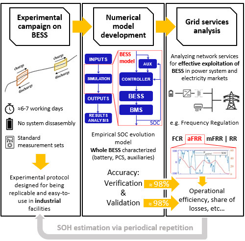
In this study, we propose the development of an experimental BESS model for SOC estimation. The model proposed aims at considering the whole system quantitatively, by implementing on a Matlab Simulink tool the relevant empirical parameters describing the performance of the battery pack, PCS, and auxiliaries. The model is designed for the analysis of power grid applications: It aims to support the BESS operator in planning the operation and designing the control strategy (e.g., for optimal scheduling and market bidding). On the other hand, it could support policymaking in evaluating the suitability of an electricity market design for storage [35,36,37]. It is not meant to substitute the battery BMS. The experimental campaign characterizing the model has been developed in the framework of this study. It is described in detail in order to be replicable in other facilities and for other systems. The V&V process is performed to assess the accuracy of the model. A case study is included showing how BESS performance can be analyzed with the model developed. It deals with frequency regulation in the framework of a market.

The model just described aims to overcome some weaknesses still present in BESS modeling highlighted in this paragraph. Indeed, this model implements the following main novelties.

• The proposed laboratory protocol for BESS characterization does not require expensive measurement set and allows to operate with probes at the switchboard level and not at the cell level, oppositely to the most widespread approaches [12,34,38,39]. This allows a user to replicate the experimental tests in most facilities (i.e., with commercial power analyzers) and to repeat the procedure periodically to also take into account the state-of-health (SOH) evolution of the battery (given obvious time constraints, it has not been possible to include SOH analysis in this paper).
• The entity modeled is the BESS (i.e., battery pack, PCS, and auxiliaries) and not just the battery. This is to conveniently retrieve all the losses of the system and to present the share of losses between the battery and auxiliary loads. As already mentioned, this is paramount for large-scale BESS operation but poorly mentioned in literature.
• It shows accuracy in SOC estimation as high as state-of-art ECMs [13], at the same time the computation effort and the test effort (required to build up the model) are strongly decreased.

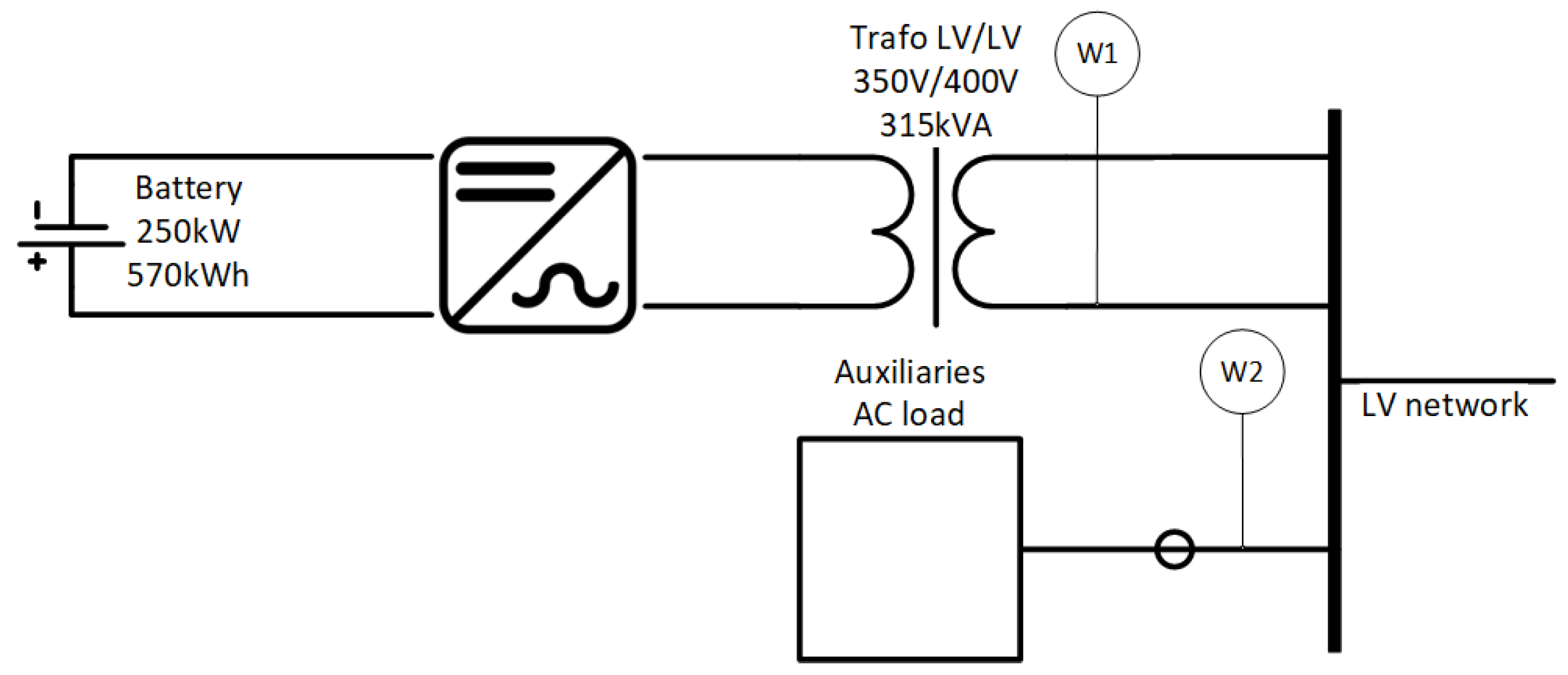
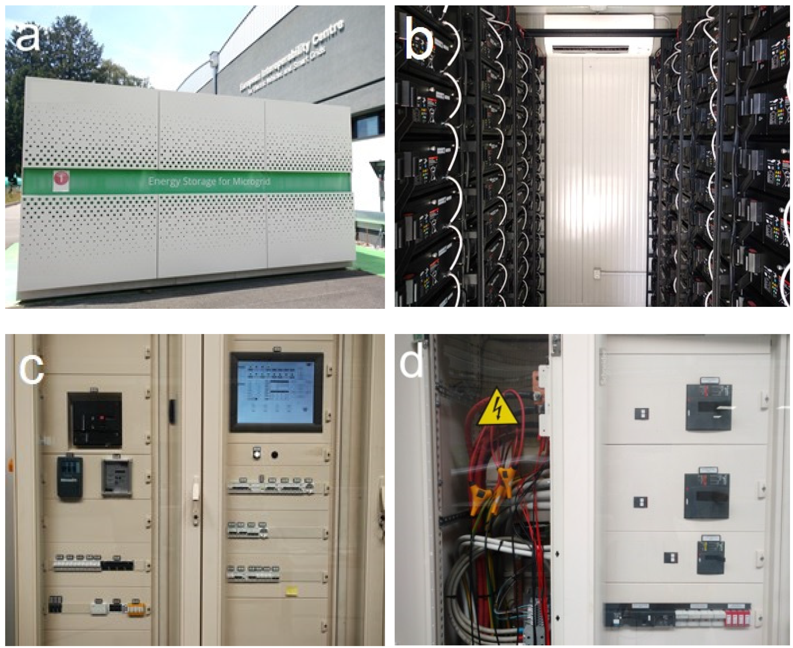
The remainder of the paper is structured as follows. Section 2 presents the set-up for the experimental campaign, including the BESS layout and the testing facility. Section 3 includes the methodology proposed for the experimental campaign, model development, V&V process, and the description of a case study in which the BESS model is used. Section 4 presents results. Section 5 contains conclusions and foreseen future steps.

2. Experimental Set-Up

2.1. The BESS Layout

The BESS tested in the experimental campaign is a Li-ion BESS for stationary application present in JRC’s Smart Grid and Interoperability Laboratory (SGILab) in Ispra (Italy) [40]. The BESS layout, shown in Figure 1, is the following one.

A Li-ion nickel-manganese-cobalt (NMC) battery pack of nominal energy (E_n) of 570 kWh and a nominal power (P_n) of 250 kW, whose datasheet is presented in

Table 1. Battery pack essential datasheet.

CELL
Technology	Li-ion NMC
Capacity [Ah]	68
Voltage Range [V]	3.1–4.1
MODULE
Capacity [kWh]	3.97
Voltage Range [V]	49.6–65.6
SYSTEM
Design Capacity [kWh]	571.9
Nominal Power [kW]	250
Cells	2304
Modules	144
Racks	12
Minimum Voltage [V]	595.2
Nominal Voltage [V]	700.8
Maximum Voltage [V]	787.2
Nominal Current [A]	357.0

. The system was installed in an external container (see Figure 2a) and was made up of 144 battery modules clustered in 12 racks (Figure 2b). The system had a DC-side protection switchboard. At the end of life (EoL), the BESS is guaranteed for a minimum E_n,EoL and P_n,EoL of 450 kWh and 225 kW.

The laboratory contained an inverter featuring a nominal power of 330 kVA. It was employed for the DC/AC conversion in low voltage (LV) from max 1200 VDC to nominal 350 VAC. A three-phase transformer in the laboratory provided galvanic separation. Its nominal power was 315 kVA. It performed the LV/LV conversion from 350 to 400 V for the connection to a three-phase busbar. A set of auxiliary AC loads was used to enable the monitoring of the BESS (via SCADA, see Figure 2c) and keeping the setpoint ambient conditions stable (e.g., the air conditioning of the battery container). The battery container featured a commercial air conditioner and heat pump operating at a setpoint temperature of 18 °C. This was kept constant throughout the year. Therefore, batteries were kept in a constant, ideal ambient condition.

2.2. Testing Facility

The operation of the BESS was followed via the local SCADA, and by some specific measurement instruments that complemented the setup of the experiment. Within the framework of this study, the commercial BESS was used in its current state, without modifying its hardware configuration. The rationale behind this was being able to guarantee a certain degree of accuracy, suitable for the application, without requiring long or expensive procedures. The built-in SCADA of the BESS returned minute-based data logs of many DC-side quantities. Specifically, SOC estimation and voltages DC-side were reported. By datasheets, the measurements by the SCADA have low accuracy and thus were processed by proprietary algorithms developed by the manufacturers. The proprietary algorithm just mentioned, unknown by the authors in its entirety, estimates the SOC based on measurements of open-circuit voltages (OCV) and energy flows. We used a Fluke 437-II analyzer [41] for gathering the AC-side measurements with a second-based sampling rate and therefore higher accuracy than the original SCADA. The sensors were connected at the busbar level (see Figure 2d) to the main BESS feeder (between the transformer and the LV bus, see Figure 1, meter W1). Another analyzer, a Fluke 1732 [42], measures the auxiliaries’ feeder (see Figure 1, meter W2). The measurements are done with branded voltage and current clamps. A temperature probe measured the ambient temperature in the surroundings of the battery container. A summary of the equipment, measurements, and accuracies estimated is presented in

Table 2. Metadata of relevant measured quantities [41,42].

Quantity	Source	Unit of Measure	Expected Range	Accuracy
Cell DC voltage	SCADA	V	[3.00–4.12]	±0.05 V
System DC voltage	SCADA	V	[595.2–787.2]	±10 V
System DC current	SCADA	A	[−400–400]	±1.0 A
SOC	SCADA	%	[0–100]	Estimation
AC voltage	Analyzer 1	V	[390–410]	±0.04 V
AC current	Analyzer 1	A	[−630–+630]	±1.0 A
AC power	Analyzer 1	kW	[−250–+250]	±0.5 kW
Auxiliaries’ power	Analyzer 2	kW	[0–10]	±0.05 kW
Network frequency	Analyzer 1	Hz	[49.8–50.2]	±0.001 Hz
Outdoor temperature	PT100	°C	[0–50]	±0.1 °C

. Such equipment had been selected as a standard measurement kit available in every facility, i.e., the goal of the paper is to propose an industrially viable approach to characterize a BESS and validate the accuracy of the procedure in a real-life implementation context.

3. The Proposed Methodology

In this section, we describe in detail the procedure followed in the experiment, so to allow the replication of the process. The goal of this study is to develop a BESS numerical model suitable for analyzing power grid applications. These include, for instance, ancillary services provision, congestion management, and RES integration and support. The model developed is an empirical SOC evolution model with lumped elements characterized by parameters estimated via an experimental campaign. The experimental campaign is presented in the next paragraph. The main elements of the BESS model implementing the parameters are described in the following.

A Controller implements the BESS operation strategy in runtime. Its inputs are real-world data or data of the user’s choice. The output is a power setpoint requested from the grid to the BESS (P_gridAC, AC-side). The sampling rate of the output can be configured and depends on the user’s choice. A key objective is to fulfill the requirement that the analysis of grid-tied applications requires, i.e., second to hour sampling rates for analyzing services with second to hour timescales.

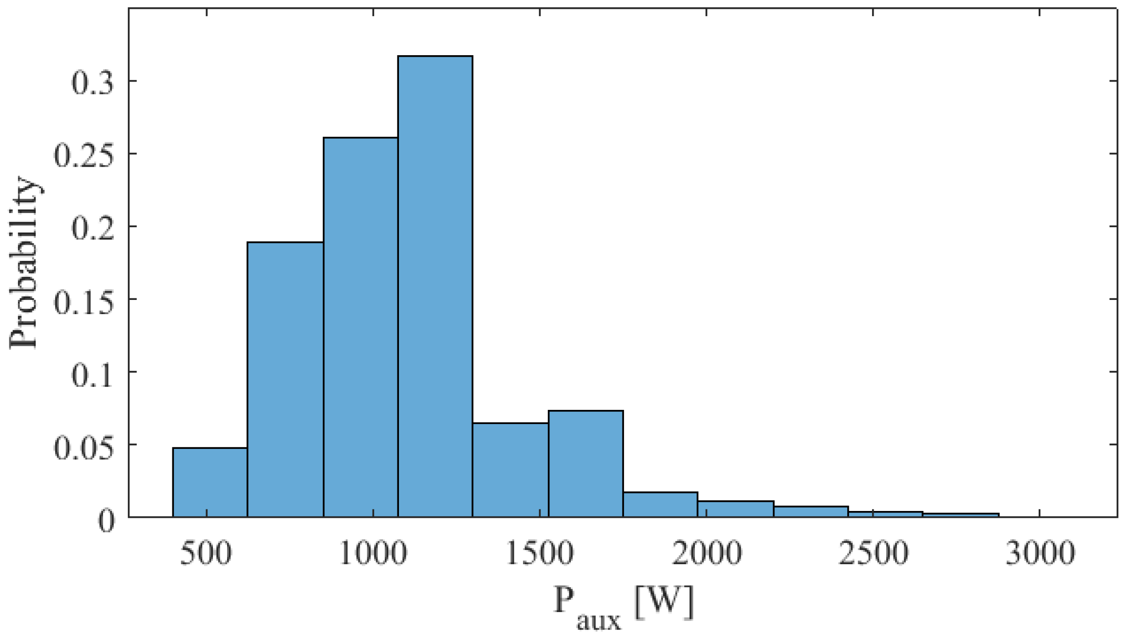
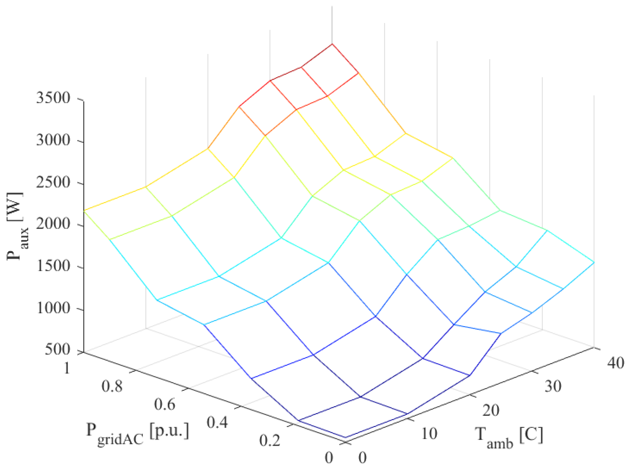
Auxiliaries’ are modeled as a load variable with respect to P_gridAC and outdoor ambient temperature (T_amb). Indeed, since the largest share of loads is related to the container air conditioning, the power requested (P_aux) heavily depends on the thermal load of the container, i.e., the thermal dissipation of batteries due to their internal electrochemical process (proportional to battery power) and the heat exchange with the ambient (proportional with T_amb).

The BESS core is composed of the PCS and the battery pack. Its overall efficiency (η_BESS) varies with P_gridAC and SOC. Given the electrochemical nature of batteries, the efficiency of the operation highly depends on the power demand and on the energy available in the battery at each instant. Our model considers an overall efficiency instead of two different efficiencies for power conversion and for battery cycling. This choice has two main purposes: (i) Decreasing the complexity of the model where possible without compromising its precision, and (ii) exploiting the higher accuracy of AC measurements. Therefore, through an experimental campaign, we compute the overall efficiency, and then the SOC is estimated based on the energy flows absorbed or injected by the BESS. The assumption made is that the battery operation is symmetrical in charge and discharge modes: i.e., η_BESS is equal in the charging and discharging processes. Furthermore, the model features a capability curve for battery active power, defining the SOC boundaries for safely delivering or absorbing different levels of power. The model described above is implemented in Matlab Simulink. This tool can simulate the runtime provision of grid services by the BESS, while considering the BESS operational efficiency, the energy flows exchanged with the network, checking the SOC, and power thresholds (the SOA). Within the framework of this study, the power setpoints proposed are given in terms of absolute power (in kW), power in per unit with respect to P_n (250 kW), and c-rate with respect to E_n (570 kWh).

3.1. The Experimental Procedure

The experimental campaign took place between March and July 2019. The proposed laboratory protocol could be split into two different test sets. The first one aims at retrieving the SOC curve with respect to the OCV of the system (SOC-OCV curve) and the capability curve of the battery. It features cycles of complete charge followed by complete discharge at constant power (DoD = 100%), as presented in

Table 3. The layout of test Set 1.

Cycle	SOCinit [%]	Active Power Setpoint [p.u.]	C-Rate [C]	DoD [%]	Estimated Elapsed Time [hours]
Cycle @ 22.5 kW	0	0.09	0.04	100	50.7
Cycle @ 45 kW	0	0.18	0.08	100	25.3
Cycle @ 90 kW	0	0.36	0.16	100	12.7
Cycle @ 135 kW	0	0.54	0.24	100	8.4
Cycle @ 180 kW	0	0.72	0.32	100	6.3
Cycle @ 225 kW	0	0.90	0.39	100	5.1

. The estimation of SOC-OCV curve is fundamental to have a reliable reference term (i.e., a state variable as OCV) for defining SOC. This allows the ability to avoid being dependent on the algorithm of SOC estimation implemented in the system by the manufacturer, which is different for each technology provider and often proprietary (i.e., unknown). Furthermore, it is recognized that a dynamic (online) estimation of SOC hardly reaches the accuracy of estimation via OCV achieved after a convenient relaxation time [43,44,45], and the SOC-OCV curve is used as a reliable reference in most methods [46,47]. Therefore, in the framework of this study, the SOC-OCV curve built as follows is used as an estimator of real SOC to be compared with SOC estimated by the model.

In the proposed protocol, the initial SOC (SOC_init) is set to 0%. To reach a SOC = 0%, the battery is discharged at constant current (CC) and then at constant voltage (CV), until the DC-bus minimum system voltage for safe operation (V = 623 V) is reached. Constant voltage discharge (that is equivalent to discharge at power decreasing up to 0 [48]) is then performed until reaching a minimum voltage with the battery idle (OCV = 623 V). It is worth noting that this voltage is higher than the minimum voltage proposed by the datasheet (see Table 1). This is because the BMS has a procedure for preventing detrimental phenomena while operating the battery. The procedure respects the requirement of a minimum settling time of 15 min before the beginning and after the end of each test. The BESS stays idle during the settling period. This ensures that the system voltage approaches a steady-state approximating OCV. After the settling time, the complete charge begins. When approaching the maximum system voltage, the BMS automatically stops the charging process. After a settling period (to identify the max OCV of the cycle), the discharging process (CC) begins. When approaching minimum system voltage, BMS stops the process. Once more, a settling period is requested to reach OCV. In order to have a full battery cycle, the final SOC must be equal to SOC_init. Therefore, if by discharging at a constant current, the battery is not able to reach the SOC_init (the initial OCV), a constant voltage discharging process is applied. All the parameters set in this procedure (e.g., the settling time) comes from a trade-off between the accuracy and the low effort requested for the procedure so it can be adopted by a BESS operator. This selection is supported by literature analysis [49,50,51]. The test steps are described in detail in

Table 4. Test steps for Set 1.

Test Step		Charge/Discharge	Stopping Criterion	Active Power
0.1	Pre-test 1: complete discharge	Discharge (CCCV)	SOC = 0%	−
0.2	Pre-test 2: settling period 1	−	Steady voltage (OCV)	−
1	Complete charge at constant power	Charge (CC)	V max reached (BMS stops the charge)	As of Table 3
2	Settling period 2	−	Steady voltage (OCV)	−
3	Complete discharge at constant power	Discharge (CC)	V min reached (BMS stops the discharge)	As of Table 3
4	Settling period 3	−	Steady voltage (OCV)	−
5	Complete discharge to 0	Discharge (CV)	Initial SOC reached	−
6	Settling period 4	−	Steady voltage (OCV)	−

.

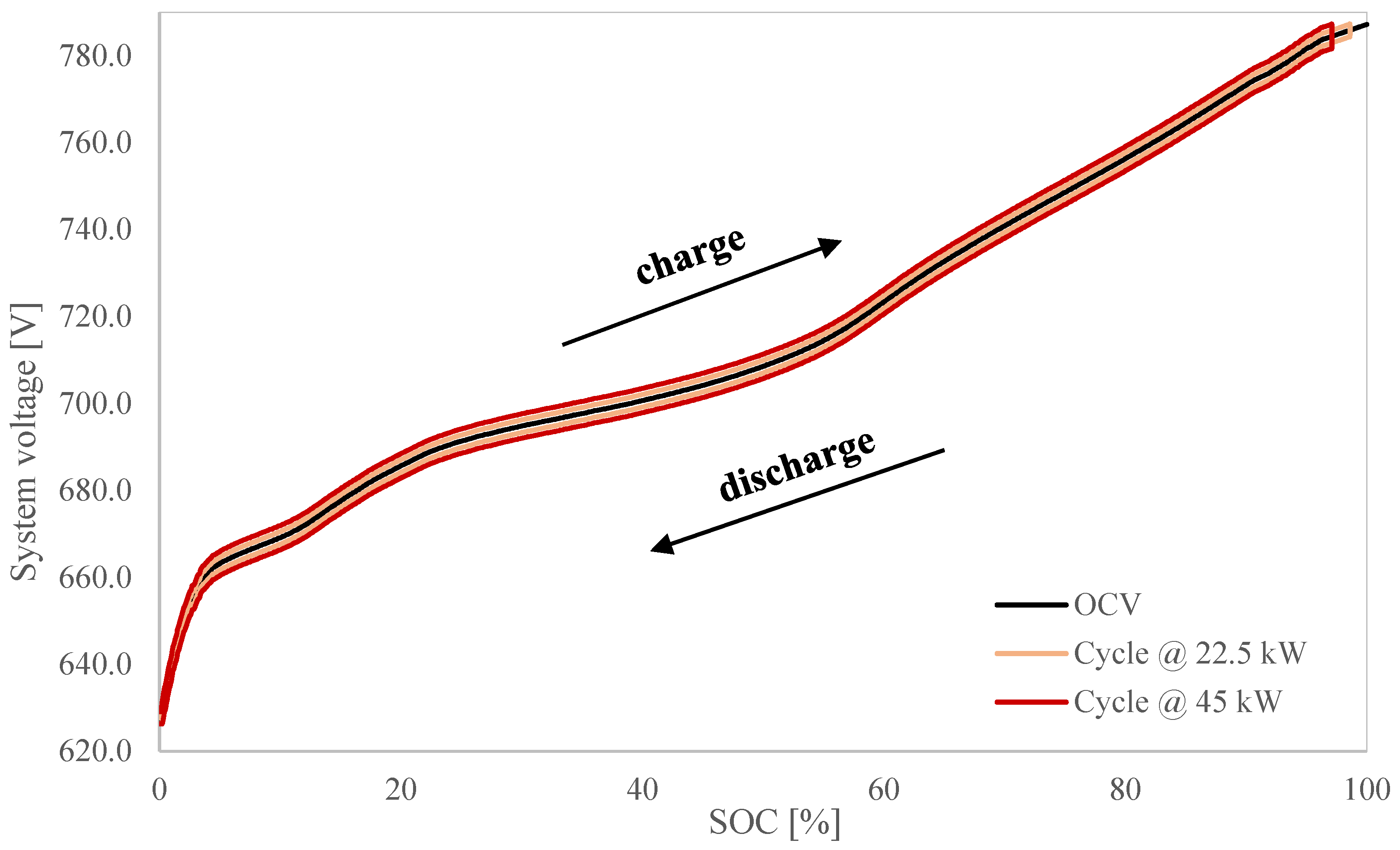
The test set includes six cycles with increasing constant power setpoints. The two tests at low power, used for building the SOC curve, are presented in Figure 3.

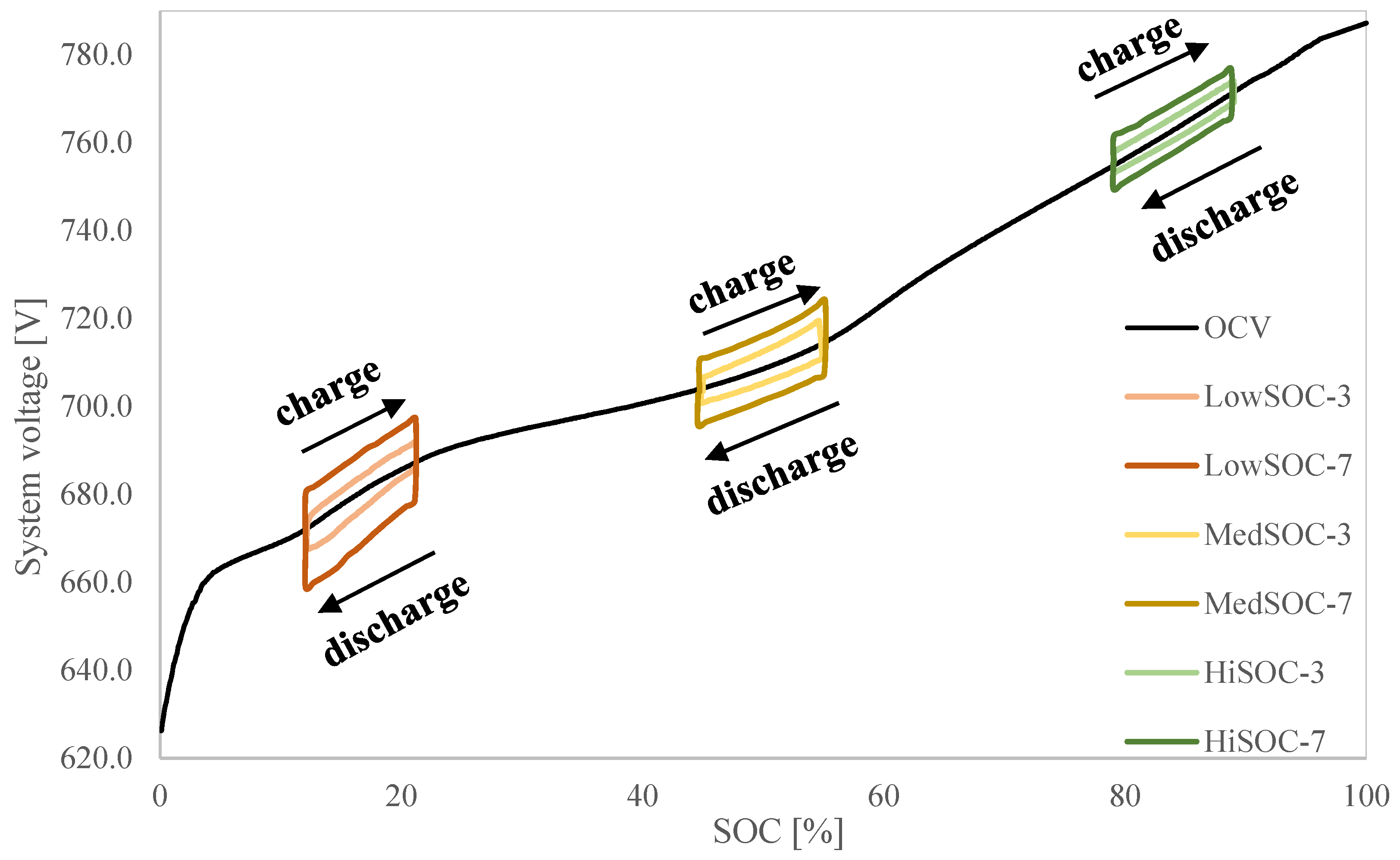
The second test set, aimed at characterizing the BESS efficiency, is presented in Table 6. The aim of this second set is to cover a large span of the possible operating conditions in terms of SOC and power requested to BESS. Again, a set of tests featuring a cycle with a charging process followed by a discharging one at constant power is proposed. In order to have a rigorous evaluation of the efficiency, each cycle is bound to have a final OCV equal to the initial one. The depth of discharge (DoD) of the cycles is limited in order to have a proper check of the cell efficiency in different operating conditions; a 10% SOC variation has been identified as the optimal trade-off between numerical accuracy and proper estimation of the efficiency in selected working condition. The steps of each test in Set 2 are described in detail in

Table 5. Test steps for Set 2.

Test Step		Charge/Discharge	Stopping Criterion	Active Power
0.1	Pre-test 1: getting to SOCinit	Charge/Discharge (CCCV)	SOC = SOCinit	−
0.2	Pre-test 2: settling period 1	−	Steady voltage (OCV)	−
1	Charge at constant power	Charge (CC)	Desired SOC reached (≈SOCinit + 10%)	As of Table 6
2	Discharge at constant power	Discharge (CC)	SOCinit approached (≈SOCinit)	As of Table 6
3	Settling period 3	−	Steady voltage (OCV)	−
4	Eventual charge/discharge to exactly reach SOCinit	Charge/Discharge (CC)	SOCinit reached (=SOCinit)	0.09 p.u.
5	Settling period 4	−	Steady voltage (OCV)	−

. A certain degree of precision in getting back to SOC_init is requested. This is not always straightforward, especially at high power. Eventually, a further charge/discharge process at low power can be operated (step 4 in Table 5). Figure 4 presents a schematic layout of the cycles in a (SOC, V) diagram.

The power setpoints are fractions of the BESS P_n, expressed in per unit through division by P_n. Each power level has been tested in three cycles, for different SOC_init: a high, an average, and a low SOC_init. The reached DoD of the cycles is approximately 10%. Exceptions (DoD lower) are made for very low power setpoints, to avoid the uncontrolled increase of the elapsed time. The minimum settling time of 15 min is also requested in this second test set.

The analyzer measures the power during both tests Set 1 and 2. Set 1 and Set 2 guarantee a satisfactory coverage of the P_gridAC range and they are designed to test a large span of T_amb (i.e., they are carried out over some months, over two seasons and both during daytime and nighttime). Indeed, since the aim is to characterize the loads during real operation, it is important to measure P_aux for T_amb ranging from 0 to 40 °C and for P_gridAC ranging from 0 (battery idle) to P_n (maximum power injected or absorbed).

3.2. Output Postprocessing and Battery Characterization

After the tests campaign, the numerical model of the BESS was characterized and implemented in the Simulink tool. This paragraph describes the data processing performed.

For characterizing the BESS design, the actual battery capacity and rated power must be estimated. In the study, E_n (in kWh) and P_n (in kW) are used. This is to better adhere to power network terminology and quantities. Test Set 1 suffices for estimating E_n. Following the definition given in [52], the battery capacity E_n is defined as the energy that can be delivered to the grid when performing a complete discharging at 20-h-rated current EoL (i_20,EoL). The choice of low current is justified by the goal of maximizing the energy that can be delivered (it is known that battery capacity decreases with power [53]). The choice of using 20-h-rated currents at EoL highlights the interest to replicate the tests at different moments during the battery life. Therefore, the data from the Set 1 cycle at 22.5 kW (450 kWh/22.5 kW = 20 h) are used as follows to compute E_n.

$${\mathrm{E}}_{\mathrm{n}}=\underset{\mathrm{dis}}{\overset{}{{\displaystyle \int }}}{\mathrm{P}}_{\mathrm{gridAC}}\left(\mathrm{t}\right)\ast \mathrm{dt}$$

(1)

where P_gridAC is integrated on time during the discharge to obtain the maximum amount of energy that can be delivered continuously to the grid. P_n is instead the maximum power allowed by the control system of the BESS.

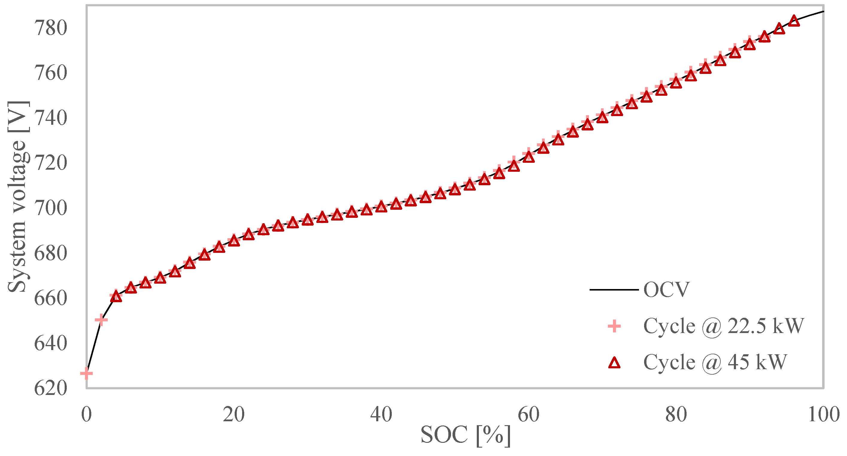
The SOC-OCV curve is obtained from the Set 1’s cycle at 22.5 kW and cycle at 45 kW. Useful data are DC current, DC voltage, and time elapsed. The SOC can be computed as follows.

$$\{\begin{array}{cc}\mathrm{SOC}\left(\mathrm{t}\right)={\mathrm{SOC}}_{\mathrm{init}}\hfill & \mathrm{if} \mathrm{t}=0\\ \mathrm{SOC}\left(\mathrm{t}\right)=\mathrm{SOC}\left(\mathrm{t}-1\right)+\frac{1}{{\mathrm{C}}_{\mathrm{n}}}\ast {{\displaystyle \int }}_{\mathrm{t}-1}^{\mathrm{t}}i\left(\mathrm{t}\right)\mathrm{dt}\hfill & \mathrm{elsewhere}\end{array}$$

(2)

where i(t) is the DC current in the interval [t − 1, t], positive if the battery is charging, and C_n is the nominal capacity, obtained as follows.

$${\mathrm{C}}_{\mathrm{n}}\left[\mathrm{Ah}\right]=\frac{{\mathrm{E}}_{\mathrm{n}}}{{\mathrm{V}}_{\mathrm{n}}}$$

(3)

where V_n is the nominal voltage (700.8 V). Therefore, we obtain a log of the SOC and the corresponding DC voltage (V_DC), from which we can build two curves of V_DC with respect to SOC while respectively charging (V_ch,cycle) and discharging (V_dis,cycle) at given powers. The SOC-OCV curve corresponding to the cycle is the average between V_ch,cycle and V_dis,cycle for each SOC.

$${\mathrm{OCV}}_{\mathrm{cycle}}\left(\mathrm{SOC}\right)=\frac{{\mathrm{V}}_{\mathrm{ch},\mathrm{cycle}}\left(\mathrm{SOC}\right)+{\mathrm{V}}_{\mathrm{dis},\mathrm{cycle}}\left(\mathrm{SOC}\right)}{2}$$

(4)

This is aiming to mitigate the hysteresis effect influence on OCV estimation [43,54]. The two SOC-OCV curves retrieved for the cycle at 22.5 kW and the cycle at 45 kW were combined to obtain the final SOC-OCV curve for the battery under testing.

$$\mathrm{OCV}\left(\mathrm{SOC}\right)=\frac{{\mathrm{OCV}}_{\mathrm{Cycle}@22.5\mathrm{kW}}\left(\mathrm{SOC}\right)+{\mathrm{OCV}}_{\mathrm{Cycle}@45\mathrm{kW}}\left(\mathrm{SOC}\right)}{2}$$

(5)

The use of both cycles decreases the possibility of transferring the inaccuracy of the DC measurements to the SOC-OCV curve. The use of cycles with lower power setpoints decreases the difference between V_ch, V_dis, and OCV for each cycle.

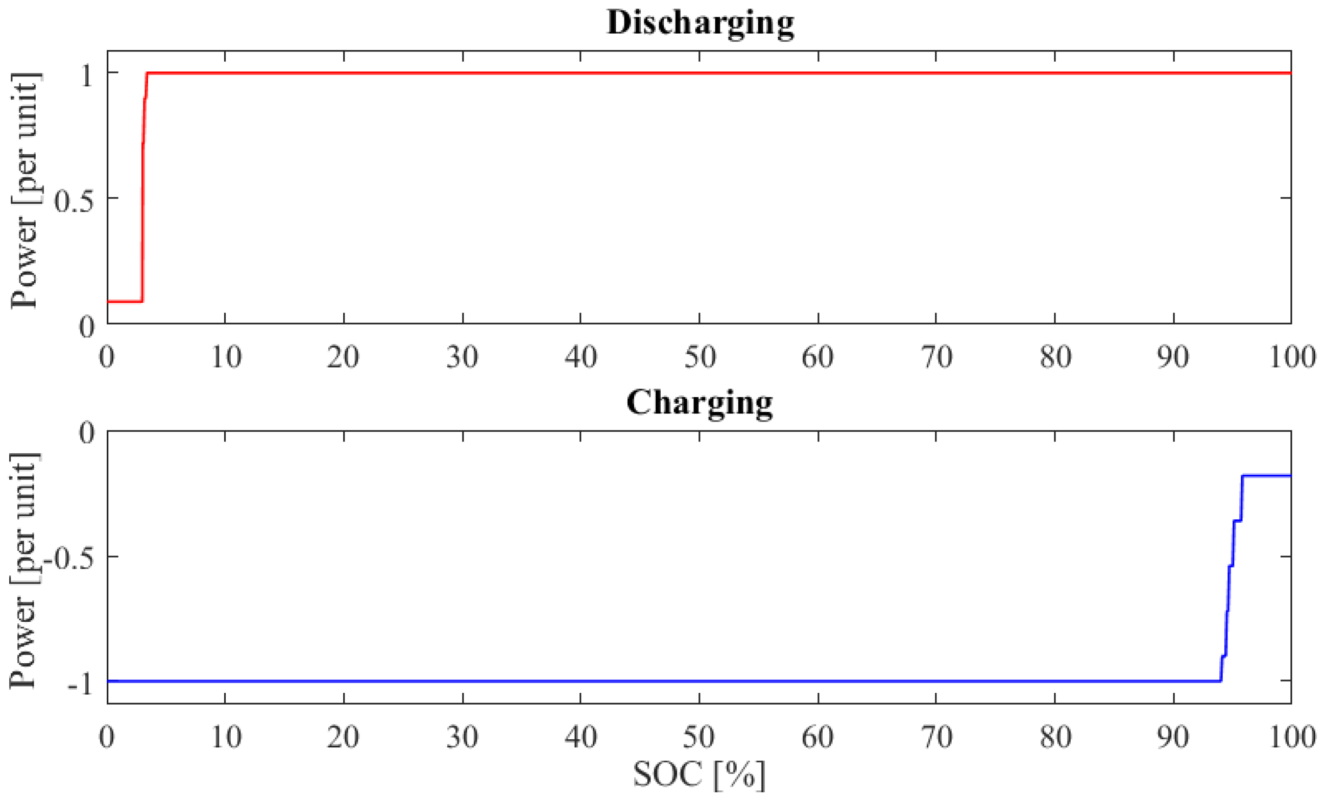
Within the framework of this study, the capability curve defines the maximum active power that can be extracted or absorbed by the BESS at a certain SOC. The BESS under testing must work within 623.0 and 787.2 V. Therefore, the BMS curtails the power setpoints obtainable outside this range (constant voltage charging/discharging). The capability curve is built by recording the OCV at the end of the charging/discharging processes in the test Set 1. When the BMS starts curtailing the power, the cycle is manually stopped and after the settling time, the OCV is recorded. Via the SOC-OCV curve, we can obtain the SOC corresponding to the OCV. This is the maximum (minimum) SOC at which a certain charging (discharging) power can be exploited. The capability curve is a way of expressing the battery capacity at a given power, different from the one used for the E_n estimation.

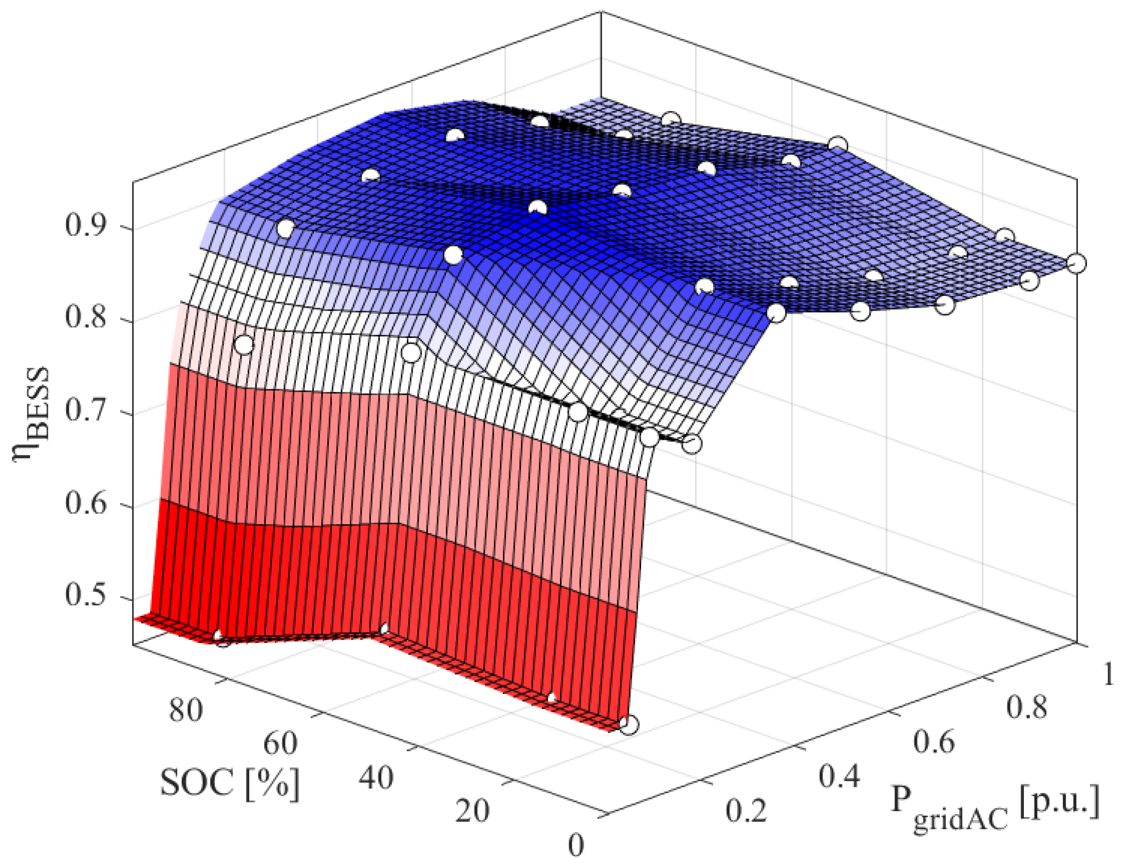
BESS efficiency (η_BESS) is estimated as a function of SOC and P_gridAC. The test Set 2 holds the data required for this. The BESS efficiency can only be computed for a whole cycle. Therefore, for each cycle of the test Set 2 we can obtain η_BESS as a function of the average power of the cycle and of the midpoint SOC of the cycle: (SOC_init + SOC_max) / 2. For each cycle of Set 2, efficiency is computed as indicated below.

$${\mathsf{\eta }}_{\mathrm{BESS}}\left(\mathrm{SOC},{\mathrm{P}}_{\mathrm{gridAC}}\right)=\frac{{\mathrm{E}}_{\mathrm{dis}}}{{\mathrm{E}}_{\mathrm{ch}}}=\frac{{{\displaystyle \int }}_{\mathrm{dis}}^{}{\mathrm{P}}_{\mathrm{gridAC},\mathrm{cycle}}\mathrm{dt}}{{{\displaystyle \int }}_{\mathrm{ch}}^{}{\mathrm{P}}_{\mathrm{gridAC},\mathrm{cycle}}\mathrm{dt}}$$

(6)

where E_dis is the energy absorbed during charge and E_ch is the energy injected during discharge, computed as the integral of power measured on the AC-side while charging or discharging.

Auxiliary power (P_aux) is registered as a function of T_amb and P_gridAC. To be sure of recording P_aux with a wide range of T_amb, measurements of the auxiliaries’ load are performed both in daytime and nighttime for an extended time period including seasonal variations (March to July 2019).

The experimental procedure developed is designed to be time effective and based on instrumentation that is normally available in each facility, i.e., it can be periodically repeated in order to take into account the state-of-health (SOH) evolution of the battery. The repetition of part or all of the procedure and the recording of new results may lead to the decision of updating the model parameters and to construct an aging model in a convenient manner. For example, just repeating the cycle at 22.5 kW in test Set 1 permits the user to analyze the capacity fade of the battery [55] in 1 working day. Repeating the entire procedure can also model the efficiency decay (i.e., the increase of internal resistance) over time [56] in approximately 6 working days. It is worthwhile to note that such tests are relevant to the evaluation of the overall BESS efficiency and capacity, moreover, they do not require the disassembly of any component. Once the procedure has been repeated, two actions are possible: If the experimental data show sensible aging, the numerical model is updated with the new parameters obtained; if the experimental data obtained are similar to the findings of the previous experimental campaign, the model does not need to be updated.

3.3. Development of the Numerical Model

The numerical model aims at accurately representing the operation of the BESS while providing grid services. The ancillary services for the electricity market of interest (such as RES support via time-shifting or balancing and energy arbitrage) are real-world cases, and therefore, the model should be capable of receiving and conveniently processing real-world input data (such as electricity market prices and quantities, dispatching signals, and weather data). 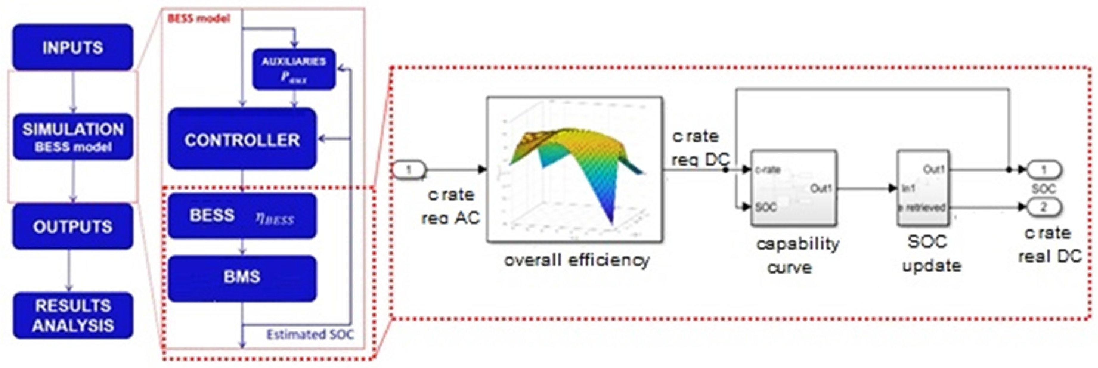Timescales of these services vary from seconds (e.g., provision of the frequency containment reserve [5]) to hours (e.g., energy arbitrage [57]). Hence a requirement for the model is to perform runtime simulations in all those timescales. The reliability of provision is of paramount importance when dealing with services to power networks. Therefore, the model must provide accurate estimates even when the BESS operates at its limits, i.e., power and SOC saturation limits. This will enable the coherent evaluation of the gap between the performance requested from the grid-side and the actual provision of the BESS (e.g., in terms of energy provided on energy requested). Given these premises, the proposed layout of the model is presented in Figure 5, to the left. Inputs are fed to the BESS model, featuring a controller implementing the control strategy for the provision of grid-related services. While developing the control strategies, the controller takes into account the presence of electric loads acting as auxiliaries of the operation. The output of the controller is a power setpoint fed to the BESS empirical model, which is characterized by η_BESS (considering both the PCS and battery pack), the capability curve, and the SOC evolution model. The outputs are the power requested DC-side and the updated SOC. These are fed to a simplified battery management system (BMS) that modifies the inputs conveniently for staying within the operational boundaries (safe operating area [58]). The main outputs of the model are the SOC and the power provided AC-side. This process is repeated for each timestep of the simulation. The outputs are elaborated for supporting the analysis of the results. The model is implemented in the already described Matlab Simulink tool, whose zoomed-in flowchart for the BESS and BMS sections are presented in Figure 5.

3.3.1. Characterization of the Model

The model implements the parameters obtained as outcomes from the experimental campaign. E_n and P_n are given as input to the simulation. They are useful in the construction of the control strategy since it is convenient to define the power setpoints as a function of P_n (in per unit). In addition, the model uses both power setpoints and c-rates, and the energy-to-power ratio (EPR) is used to transform between these two quantities. The auxiliaries’ power demand is schematized in a 2-D lookup table (LUT) with P_gridAC and T_amb on the x- and y-axis. η_BESS is returned as a 2-D LUT with a c-rate and SOC on an x- and y-axis. The capability curve is returned as two 1-D LUT for charge and discharge, with SOC on the x-axis. The capability curve returns as output the maximum absolute value of power from the DC-side that can be delivered, for both charge and discharge.

3.3.2. The BESS Controller

An in-depth development of the controller is outside the scope of this study. Within this framework, the controller is only used for:

• directly receiving the power setpoints (P_gridAC) from input time-series. This occurs during the verification, where the BESS model must operate on a cycle of the user’s choice;
• converting frequency deviation in a power setpoint via a droop control curve. This occurs during the validation process, where the BESS model is tested via frequency regulation cycles.

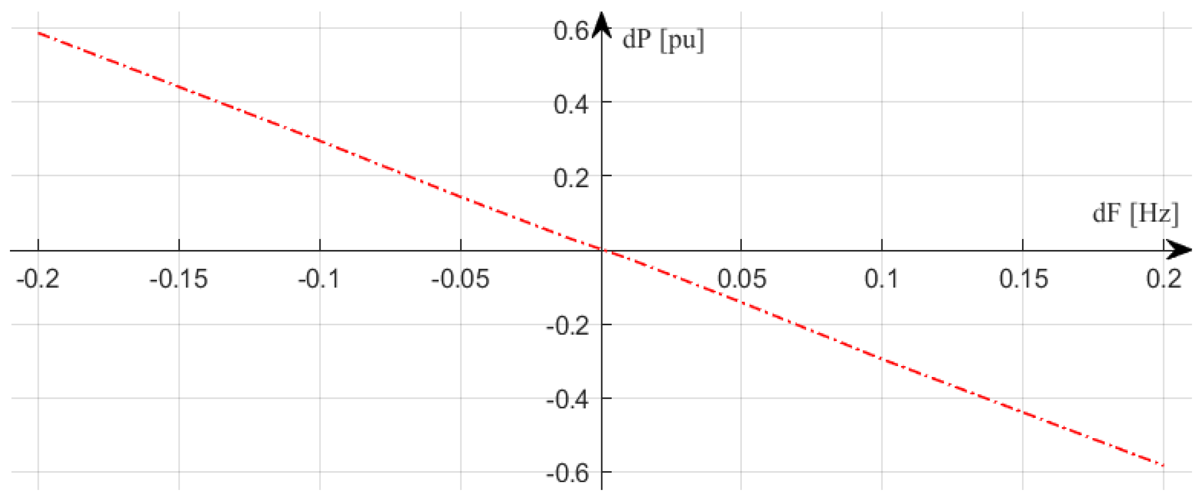
The droop control curve is built in the model controller based on the curve controlling the operation of a real battery under study while providing frequency regulation. It is a simplified control curve, defined in Equation (7) and presented in Figure 6, featuring no dead band and a droop value of 0.69%, computed as follows:

$$\mathrm{droop}[\%]=\frac{\frac{\mathrm{dF}}{{\mathrm{F}}_{\mathrm{n}}}}{\frac{\mathrm{dP}}{{\mathrm{P}}_{\mathrm{n}}}}\ast 100$$

(7)

where dF is frequency deviation (in Hz), F_n is network nominal frequency of 50 Hz, dP is the power setpoint (in kW) and P_n is nominal power of BESS (in kW).

3.4. Model Verification and Validation

The development of a model must include tests for verifying how accurately it represents the simulated system. The verification process verifies if the model is built using the correct equations and if there are no errors in its structure. The validation process aims at defining if the model is appropriate for the foreseen application [32,33].

Verification includes debugging the code for checking material errors and running tests capable of covering and checking the majority of the domain in which the model moves. This means, for the BESS model we are building, testing the behavior of the model with different couples of SOC and power setpoints requested from grid (SOC and P_gridAC). Indeed, the main parameter η_BESS is a function of these two variables. Validation includes testing the model on real-world data related to the model destination—grid-tie applications. Adopting typical timescales and power demand patterns of the phenomena under study is fundamental for validation.

3.4.1. Verification Procedure Proposed

The rationale behind the proposed verification procedure is preventing all possibilities of error during coding and verifying that the model is simulating the system with proper accuracy on a large coverage of the possible operating conditions. These include different power demand to BESS (ranging from −250 to 250 kW) and several SOC conditions (ranging from 0% to 100%).

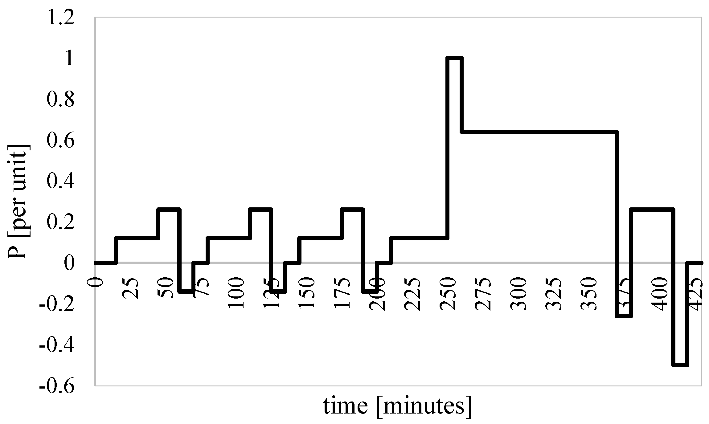
We coded the Simulink tool implementing the model using modular programming. Operating this way, we obtain defined units in which we can scope intermediate inputs and outputs, comparing them with manual calculations [33]. Furthermore, the verification includes running a test built based on the standard IEC 62660-1 taken from literature [59,60]. The IEC standard applies to the performance testing of Li-ion batteries for the propulsion of electric road vehicles rather than for stationary applications. Despite this, it has been selected for its large coverage of the domain of interest. Some modifications were applied to the standard proposed in the framework of this study to better fit the application proposed. The power profile of the proposed cycle is shown in Figure 7. Indeed, it allows the development of a verification test on the BESS and the model under study, with DoD being almost 100% and the power profile ranging from −125 to 250 kW. An almost complete coverage of the operating conditions in terms of SOC and power requested to BESS are verified by this test.

This profile is fed to the real BESS. The model runs a simulation cycle with the same profile. Initially, the SOC was in both cases 97.5%. Outcomes are evaluated using the following metrics.

SOC estimation error during verification (e_SOC,V1) is defined as the difference between the real SOC (SOC_real) after reaching a stationary state (retrieved as a function of OCV using SOC-OCV curve) at the end of the test and SOC estimated by model (SOC_model) at the end of the simulation.

$${\mathrm{e}}_{\mathrm{SOC},\mathrm{V}1}[\%]={\mathrm{SOC}}_{\mathrm{real}}-{\mathrm{SOC}}_{\mathrm{model}}$$

(8)

This index provides an absolute figure of the error as a percentage of SOC.

Energy estimation error during verification (e_E,V1) is defined as the ratio between e_SOC,V1 multiplied by E_n and the total absolute value of energy flown during verification test, obtained integrating on time the absolute value of power injected or absorbed AC-side.

$${\mathrm{e}}_{\mathrm{E},\mathrm{V}1}[\%]=\frac{\left(\frac{{\mathrm{e}}_{\mathrm{SOC},\mathrm{V}1}}{100}{\ast \mathrm{E}}_{\mathrm{n}}\right)}{{{\displaystyle \int }}_{\mathrm{V}1}^{}\left|{\mathrm{P}}_{\mathrm{gridAC}}\right|\mathrm{dt}}\ast 100$$

(9)

This second index provides a dimensionless figure of the estimation error with respect to the total energy exchanged with the grid within a process.

3.4.2. Validation Procedure Proposed

The validation process tests the BESS in a real-world use case, consistent with the model destination. Since the case under study is the analysis of the grid-tie application of BESS, the proposed validation process features the most widespread stationary application for a grid-connected BESS, and as already mentioned, around 50% share the total electrochemical storage stationary capacity installed as of mid-2017 performs frequency regulation [4]. Specifically, a primary frequency control (PFC) provision is tested—such a frequency regulation requests fast response and has reduced timescales (power intensive) [36]. PFC is adopted for testing the model on the most stressful operating conditions. The droop control curve presented in Figure 6 is used for providing PFC. The choice of selecting a droop curve without a dead band is meant to increase energy flows during the testing, thus decreasing the test duration. This is suitable for the validation process since its purpose is to investigate the estimation error rather than the effectiveness of the control strategy.

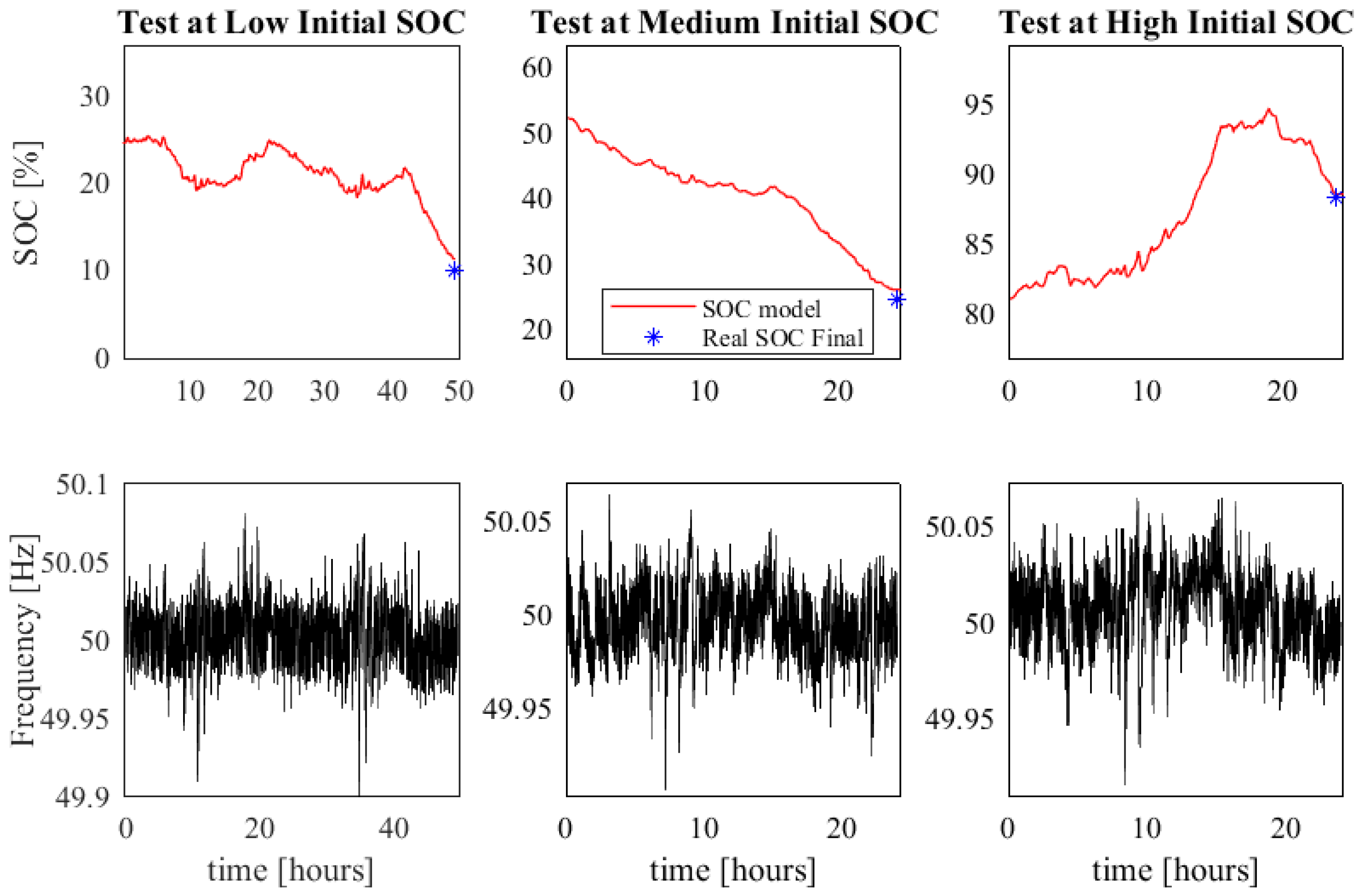
The proposed procedure includes several tests on the real BESS, then repeated using the BESS model. The real BESS measures the deviation of network frequency (f) in real-time at its connection point. It transforms frequency deviation into the power setpoint on the AC-side of the BESS via the droop equation proposed in Equation (7), with a droop value of 0.69%. For the validation test, the PFC is continuously provided for 24–48 h. The BESS model is then fed with the frequency logs returned by the testing facility. The BESS controller implements the droop curve. Therefore, the real BESS and the model provide PFC following the same 24–48 h frequency trends. Results are evaluated as for the verification process—the metrics obtained are the SOC estimation error during validation (e_SOC,V2) and the energy estimation error during validation (e_E,V2).

As a final index, the V&V procedure proposes the average hourly SOC estimation error, obtained as follows.

$${\overline{\mathrm{e}}}_{\mathrm{h},\mathrm{SOC}}[\%]=\frac{{{\displaystyle \sum }}_{\mathrm{i}=1}^{\mathrm{N}}\left(\frac{\frac{\left|{\mathrm{e}}_{\mathrm{SOC},\mathrm{i}}\right|}{100}}{{\mathrm{t}}_{\mathrm{i}}}\right)}{\mathrm{N}}\ast 100$$

(10)

where e_SOC,i is the SOC estimation error of test i, t_i is the duration of test i in hours and N is the number of tests considered. This index represents the absolute value of the SOC estimation error the model could make on average during a 1-hour long simulation.

3.5. Case Study

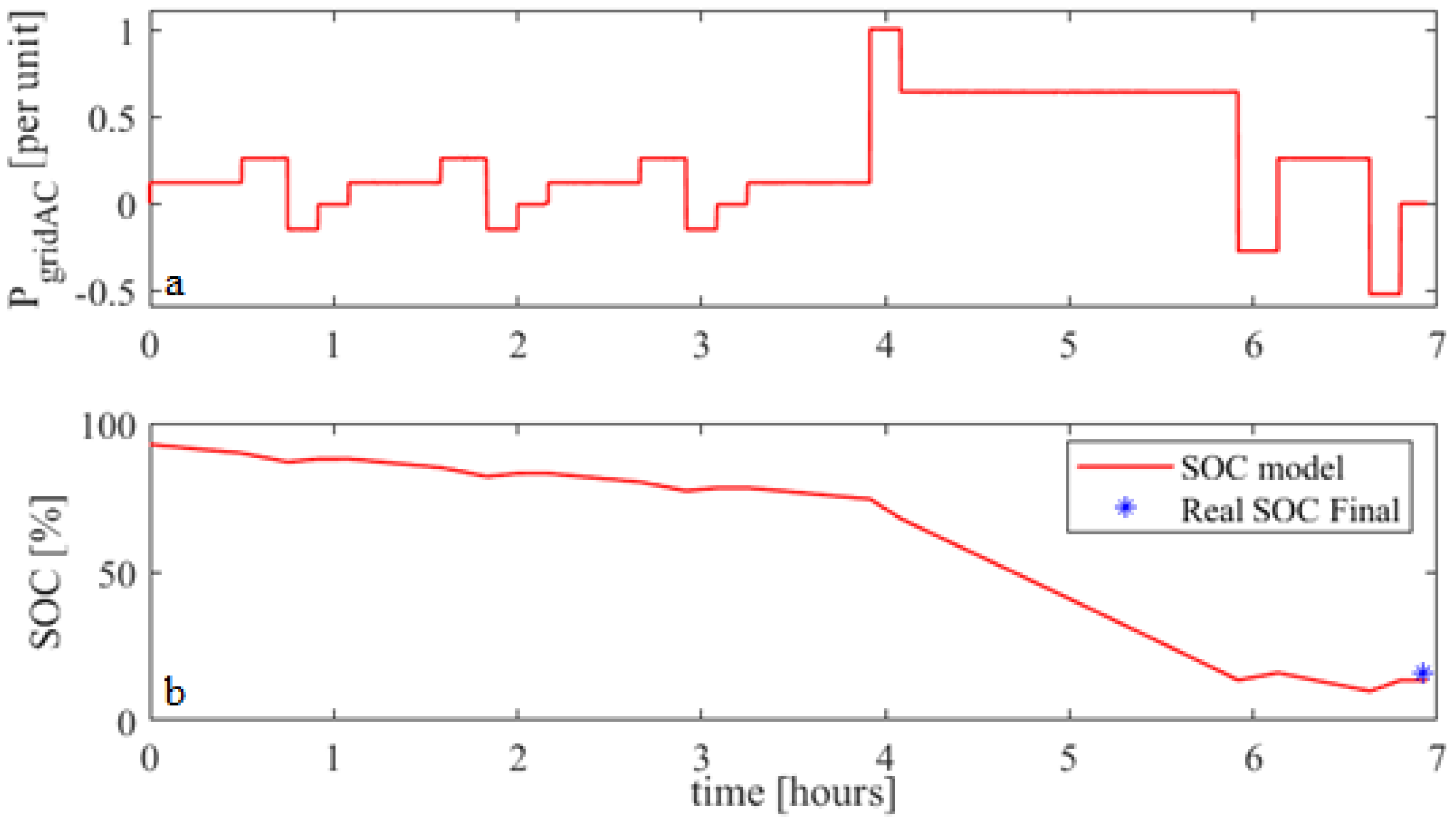
After V&V, the model is used for the analysis of BESS operation. The case study is presented for showing a potential application of the model on the Italian market. The case study aims to analyze the performance of BESS while providing frequency regulation. The V&V process focused on PFC to test the fast response. The PFC is not market-based in Italy, since it is mandatory for large-scale conventional power plants [61]. It must, therefore, be provided permanently by these units. Secondary frequency control (SFC) is instead traded on the ancillary services market (ASM) in Italy. It is the control strategy aiming at providing automatic frequency restoration reserve (aFRR). 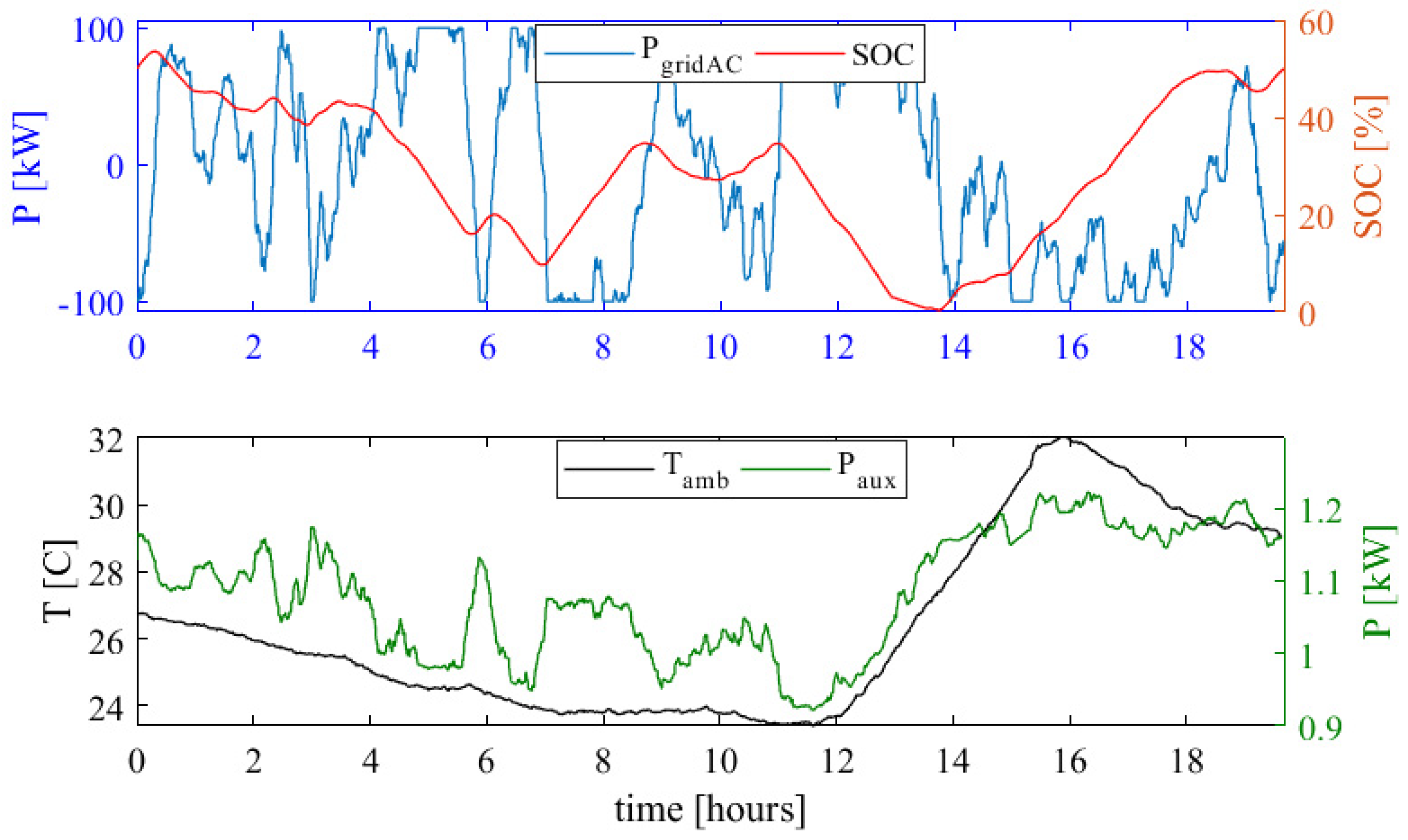A market player willing to provide aFRR in Italy would have to participate in auctions on the Italian ASM with a contracted period of 4 h and a distance from gate closure to delivery time of about 1 hour and 30 min [62]. Thus, a 5 h 30 min simulation would be suitable for analyzing the battery operation throughout one market session for an aFRR provision. The case study proposes a simulating period of about 20 h, in order to review the performance for a BESS operating in several market sessions (4 sessions).

The BESS is supposed to participate in Italian ASM and always be selected on June 22, 2019. The relevant KPIs in this case study are the efficiency of operation and the share of losses between battery, PCS, and auxiliaries. The KPIs are computed as follows:

$${\mathsf{\eta }}_{\mathrm{global}}=\frac{{\mathrm{E}}_{\mathrm{dis}}}{{\mathrm{E}}_{\mathrm{ch}}+{\mathrm{E}}_{\mathrm{aux}}}=\frac{{{\displaystyle \int }}_{\mathrm{dis}}^{}{\mathrm{P}}_{\mathrm{gridAC}}\mathrm{dt}}{{{\displaystyle \int }}_{\mathrm{ch}}^{}{\mathrm{P}}_{\mathrm{gridAC}}\mathrm{dt}+{\displaystyle \int }{\mathrm{P}}_{\mathrm{aux}}\mathrm{dt}}$$

(11)

$${\mathsf{\eta }}_{\mathrm{battery}+\mathrm{PCS}}=\frac{{\mathrm{E}}_{\mathrm{dis}}}{{\mathrm{E}}_{\mathrm{ch}}}=\underset{\mathrm{ch}}{\overset{}{{\displaystyle \int }}}{\mathrm{P}}_{\mathrm{gridAC}}\mathrm{dt}$$

(12)

$${\mathrm{loss}}_{\mathrm{global}}=1-{\mathsf{\eta }}_{\mathrm{global}}$$

(13)

$${\mathrm{Share}\mathrm{of}\mathrm{losses}}_{\mathrm{battery}+\mathrm{PCS}}[\%]=\frac{1-{\mathsf{\eta }}_{\mathrm{battery}+\mathrm{PCS}}}{{\mathrm{loss}}_{\mathrm{global}}}\ast 100$$

(14)

$${\mathrm{Share}\mathrm{of}\mathrm{losses}}_{\mathrm{aux}}[\%]=\frac{{\mathsf{\eta }}_{\mathrm{battery}+\mathrm{PCS}}-{\mathsf{\eta }}_{\mathrm{global}}}{{\mathrm{loss}}_{\mathrm{global}}}\ast 100$$

(15)

where P_gridAC is the power requested to BESS for aFRR provision, P_aux is the auxiliaries’ demand. It is important to recall that efficiencies (and therefore losses) can be computed only in case the test performs a battery cycle (SOC at the beginning equals SOC at the end of test), as it is in the case study. Indeed, the exact duration of the test allows the ability to show a complete battery cycle. The data fed as input to the model are real-world data for June 22. The power setpoint data centrally dispatched by the Italian TSO for aFRR provision are available at [63]. Ambient temperature is recorded via PT100 on-site. The model sampling rate is 1 s.

4. Results

This section presents the results related to the characterization of the model via the experimental campaign, and to the evaluation of the model via the V&V process. These results enable us to systematically describe the performance of the Li-ion large-scale BESS and the modeling tool developed for this study.

4.1. Model Parameters

The model parameters obtained as described in Methods are E_n, P_n, SOC-OCV curve, capability curve, η_BESS, and P_aux.

4.1.1. Nominal Energy and Power

The nominal energy obtained as an outcome of test Set 1 is

$${\mathrm{E}}_{\mathrm{n},\exp }=570.0\mathrm{kWh},$$

(16)

available on the AC side discharging at 22.5 kW of constant power output. The value obtained is coherent with the declared E_n.

P_n is directly set by the BESS control system:

$${\mathrm{P}}_{\mathrm{n},\exp }=250.0\mathrm{kW}$$

(17)

P_n is reached in both charge and discharge process.

4.1.2. State of Charge-Open Circuit Voltage Curve

The SOC-OCV curve of the BESS was built within Set 1 and is presented in Figure 8. Two curves had been built (via the cycle at 22.5 kW and the cycle at 45 kW) and meshed to increase the overall reliability. Some obstacles were met while dealing with the SOC when close to saturation at 0% and 100%. The BMS sometimes acted in advance (triggered by transient voltages) and prevented the SOC from reaching the upper and lower boundaries. Therefore, the upper and lower tail of the OCV curve can present a lower degree of accuracy. Figure 8 presents both the final OCV curve (black line) and the different experimental evidence for Set 1’s cycles (pink + and red triangles).

As can be seen, the experimental curves built are almost overlapping. Therefore, the estimation is considered reliable. Within the framework of this study, the real SOC is obtained by adopting this curve as reference.

4.1.3. Capability Curve

The model implements a capability curve for BESS for active power only. As described before, the Set 1 tests are analyzed for building the curve. Since these tests comprise both the CCCV charge and discharge processes, the capability curve is built at the end of a constant current process. The curve is presented in Figure 9. It represents the maximum charging and discharging power achievable for each SOC.

4.1.4. BESS Efficiency

The overall storage and conversion process efficiency is the main outcome of the experimental campaign. As already described, η_BESS is computed as a function of P_gridAC and SOC. It is obtained as an outcome of the test Set 2. BESS efficiency is the ratio between energy injected and energy absorbed within a cycle. The surface of η_BESS is presented in Figure 10, obtained via the linear interpolation of the experimental outcomes on the domain.

The system efficiency is generally high (around 90%). η_BESS heavily depends on power requested to the battery—at low power, PCS losses become predominant and efficiency sharply decreases. At high power, the inefficiencies related to phenomena inside the electrochemical cells lead to mildly lower efficiency. Fixing the power, the SOC close to 50% presents with a η_BESS slightly higher. Efficiency is implemented in the model as a LUT. The LUT is presented in

Table 7. BESS efficiency lookup table as implemented in the model.

ηBESS	SOC [%]
PgridAC [per unit]		0	15	50	85	100
	0.00	0.540	0.540	0.550	0.480	0.480
	0.05	0.540	0.540	0.550	0.480	0.480
	0.09	0.842	0.842	0.842	0.787	0.787
	0.18	0.818	0.818	0.931	0.896	0.896
	0.36	0.926	0.926	0.947	0.917	0.917
	0.54	0.895	0.895	0.931	0.927	0.927
	0.72	0.868	0.868	0.922	0.908	0.908
	0.90	0.861	0.861	0.896	0.859	0.859
	1.00	0.861	0.861	0.896	0.859	0.859

.

4.1.5. Auxiliaries’ Power

BESS rely on a set of auxiliary loads for operating. Conveniently estimating the weight of P_aux is fundamental for analyzing BESS operation and performance. Set 1 and Set 2 allowed the ability to measure P_aux in a vast range of operating conditions, in terms of ambient temperature (T_amb), and power requested to BESS (P_gridAC). The measurements were processed to obtain a minute-based average P_aux. The probability distribution of these values is reported in Figure 11. The total number of observations is 9466 (i.e., 9466 min of BESS operation were analyzed).

Based on these measurements we built the 2-D LUT presented in Figure 12 and

Table 8. Auxiliaries’ power lookup table as implemented in the model.

Paux [W]		PgridAC [kW]
		0	45	90	135	180	225	250
T [°C]	0	558	567	874	1322	1423	1950	2188
	10	558	567	874	1322	1423	1950	2188
	20	733	742	1050	1497	1598	2125	2363
	25	1092	1004	1408	1856	1957	2483	2721
	30	1197	1253	1683	2024	2125	2652	2890
	35	1341	1412	1703	2045	2146	2672	2910
	40	1516	1704	1749	2180	2281	2807	3045

. In the LUT, we only reported the average value for the observation in the surrounding of each point (T_amb and P_gridAC). This was feasible since the model aims at representing the energy demand while disregarding the power profile. This latter is influenced by duty cycles of the appliances whose representation is out of the scope of this study. As can be seen, a slice of the auxiliaries’ power (around 1000 W) is always present, feeding the components that are continuously operating in normal conditions and even with the battery idle (e.g., monitoring systems, SCADA, and alarms). In addition, there is a strong direct proportionality between P_aux and P_gridAC—parts of the loads are directly related to the BESS operation (e.g., PCS fans). Eventually, P_aux increases with T_amb, due to the need for the air conditioning of the battery container.

4.2. Validation and Verification of the Model

Results of the V&V processes are presented in the following paragraph. For what concerns verification, the performance of the model in approximating the real BESS was evaluated by the already introduced cycle based on the IEC 62660-1 performance test. A summary of the verification test is presented in

Table 9. Verification test summary.

TEST DATA
Starting date and time	July 4, 2019. 8:45 a.m.
Elapsed time	6 h 4 8m
Initial OCV [V]	777.5
Initial SOC [%]	92.80
Final OCV [V]	679.0
Final SOC [%]	15.75
Total energy exchanged [kWh]	540.11
MODEL PERFORMANCE
Simulating time	≈10 s
Initial SOC	92.80
Estimated Final SOC	13.46
${\mathit{e}}_{\mathit{S}\mathit{O}\mathit{C}\mathit{,}\mathit{V}1}[\%]$	−2.29
${\mathit{e}}_{\mathit{E},\mathit{V}1}[\%]$	−2.42

. Both e_SOC,V1 and e_E,V1 are below 2.5%. The model estimates a final SOC approximately 2% lower than the actual one.

The trend of SOC estimated by the model is presented in Figure 13. As can be seen, the test included a large range of SOC values, from 92.8% to 9.8%. The large coverage of the model domain (in terms power and SOC) enhances the robustness of the verification test.

The validation process was performed via a series of tests in which the BESS was delivering PFC. We present the results of three of them and a general evaluation of the process. The three tests presented in Figure 14 are selected for analyzing SOC estimation when providing PFC starting from low, medium, and high SOC.

Diagrams show the SOC evolution in the model and the comparison with respect to the SOC retrieved by the SOC-OCV curve at the end of the test (blue stars). A summary of the results of validation tests is shown in

Table 10. Validation tests summary.

Test Data	Low SOC	Medium SOC	High SOC
Starting date and time	July 15, 2019. 12:23 p.m.	June 14, 2019. 2:51 p.m.	June 16, 2019. 2:34 p.m.
Elapsed time	49 h 24 m	24 h 40 m	24 h 30 m
Initial OCV [V]	690.90	710.80	757.90
Initial SOC [%]	24.40	52.10	80.95
Final OCV [V]	669.00	690.90	770.20
Final SOC [%]	9.80	24.40	88.25
Total energy exchanged [kWh]	526.16	254.78	293.88
MODEL PERFORMANCE	Low SOC	Medium SOC	High SOC
Simulating time	≈20 s	≈15 s	≈15 s
Estimated Final SOC	11.14	25.79	88.43
${\mathit{e}}_{\mathit{S}\mathit{O}\mathit{C},\mathit{V}2}[\%]$	1.34	1.39	0.18
${\mathit{e}}_{\mathit{E},\mathit{V}2}[\%]$	1.45	3.11	0.35

.

The errors in the 24-hours PFC provision tests are always lower than 5%, both in terms of absolute SOC error, and of error on total energy delivered. Within the whole V&V process, on a total of 10 tests (N = 10 in Equation (10)), we also computed the average hourly SOC estimation error ${\overline{e}}_{h,SOC}$, proposed in

Table 11. Average hourly SOC estimation error.

	Average Value [%]	Standard Deviation [%]
${\overline{\mathit{e}}}_{\mathit{h},\mathit{S}\mathit{O}\mathit{C}}$	0.168	0.145

.

The general performance shown by the model is accurate. The accuracy is always more than 95% (with an average of 98%) both during verification and validation, in terms of estimation of energy flows, i.e., as complementary to one both of e_E,V1 and e_E,V2. Regarding accuracy concerns in the SOC estimation, we focused on the average hourly error ${\overline{e}}_{h,SOC}$. For a better understanding of this index, a link with real-world situations is proposed in the following case study.

4.3. Case Study: Analysis via the Model of the Operation of BESS as an aFRR Provider

The automatic frequency restoration reserve (aFRR) is one of the main ancillary services traded in electricity markets. In Italy, the aFRR is provided by the SFC [61]. The outcomes of the test on the aFRR provided for one day following Italian regulatory framework is presented. The BESS model’s accuracy on SOC estimation expected for this case study is reported in

Table 12. BESS models’ average error in estimating SOC during a market session of the automatic frequency restoration reserve (aFRR) provision.

Simulated Time [h]	20
Expected Accuracy [%]	96%

as the complementary to average hourly error multiplied by the simulating time period in hours (t_sim):

$$\mathrm{Accuracy}=1-\frac{{\overline{\mathrm{e}}}_{\mathrm{h},\mathrm{SOC}}{\ast \mathrm{t}}_{\mathrm{sim}}}{100}.$$

(18)

The trends of the main variables during the simulation are proposed in Figure 15. The main data of the simulation and the KPIs are presented in

Table 13. Summary of the results of aFRR provision.

Simulated Datetime		June 22, 2019. 12:01 a.m.
Time Elapsed		19 h 39 m
Service Provided		aFRR – Regolazione Secondaria [52]
Qualified Power	[kW]	100
Edis	[kWh]	579.2
Ech	[kWh]	612.4
Eaux	[kWh]	21.3
ηglobal	[%]	91.4%
ηbattery+pcs	[%]	94.6%
Share of losses
Battery + PCS	[%]	63.1%
Aux	[%]	36.9%

.

In a context of high global efficiency of operation (the roundtrip efficiency is above 90%), it is shown how the weight of the auxiliaries on the total losses is almost 40%. The weight of auxiliaries is supposed to change as a function of ambient temperature and power requested to battery.

Table 14. Overall summary of performed simulations.

Simulation Set	#Tests	Target	Coverage	Main Results
Verification	1	Test the model on a large coverage of the domain (P, ΔSOC)	Pmin,max = [−125, +250] kW SOCmin,max = [10, 93] %	Model verified (Accuracy ca. 98%)
Validation	9	Test the model on real-world operation (FCR provision)	Pmin,max = [−55, +79] kW SOCmin,max = [11, 88] %	Model validated (Accuracy ca. 98%)
Case study	1	Test a business case (aFRR provision on Italian ASM)	Pmin,max = [−100, +100] kW SOCmin,max = [4, 52] %	Operational efficiencies and share of losses

presents the summary of simulations with targets, coverage of the possible operating conditions (in terms of SOC and power), and the main outcomes of each simulation set.

5. Conclusions

The study presents the development, validation, and verification of an experimental Li-ion BESS model. The purpose of the numerical model is analyzing, for research and commercial purposes, the operation of BESS during the provision of services to networks in a grid-tie configuration. The possible services include, but are not limited to, ancillary services, energy arbitrage, and integration of RES in the electricity markets. Therefore, a good degree of accuracy is requested. In any case, the proposed procedure aims at improving the efficiency—in terms of time and equipment—of the required experimental campaign. Some limitations or approximations are accepted in order to provide a procedure applicable by the BESS operator with reasonable timing and effort. The model offers a trade-off between precision of the estimation and low computational effort. This latter point is not secondarily important when considering testing over long periods or in the case of serial testing of control strategies. The error recorded during the V&V processes was always below 5% for a 24-hour test. The authors consider this result acceptable for the purposes foreseen and in line with examples from literature [13], mainly featuring ECMs. Accuracy around 98% is shown by the model both in terms of SOC and energy flows estimations while validating it on frequency regulation provision. Usually, model accuracy is tested on standard charge/discharge cycles [16]. This could hinder the investigation of BESS behavior in real-world operation—this issue is overcome with the approach proposed in this paper, with a strong validation campaign featuring frequency regulation provision. The high accuracy in SOC estimation during grid-connected operation is achieved by an empirical model with a low degree of complexity—the battery is characterized by two main parameters (efficiency and capability curve). This kind of model requires a simulating time that can be 20–50 times smaller than the simulating time for ECMs [15,18]. In addition, this model does not disregard the complexity of the BESS—the auxiliaries’ power demand is modeled as a function of ambient temperature and power requested to the battery. This is an innovation for BESS modeling, since auxiliaries are poorly mentioned in scientific publications [20].

Furthermore, a case study analyzing BESS performance as a provider of the aFRR in the Italian market is presented. Specifically, the share of losses in operation between battery, PCS, and auxiliaries is estimated as a KPI. The large weight of auxiliaries over the total losses justifies and strengthens the motivation behind the development of such an organic BESS model.

During the experimental campaign, issues deriving from the use of proprietary algorithms such as SOC estimation and safe operating area implementation by BMS were met. This led to some uncertainties when describing the battery operation at very high or very low SOC (0–2%; 97–100%).

Future works on this model are foreseen. The main activity stream will focus on the development of the model controller. We expect to implement control strategies for the operation of BESS in markets, and in general for operating grid-connected BESS. Then, the operation of BESS will be analyzed both in terms of technical and economic performance, based on the definition of KPIs.